Figure 1.
Illustration of the HMF 2020K4 loader crane.
Figure 1.
Illustration of the HMF 2020K4 loader crane.
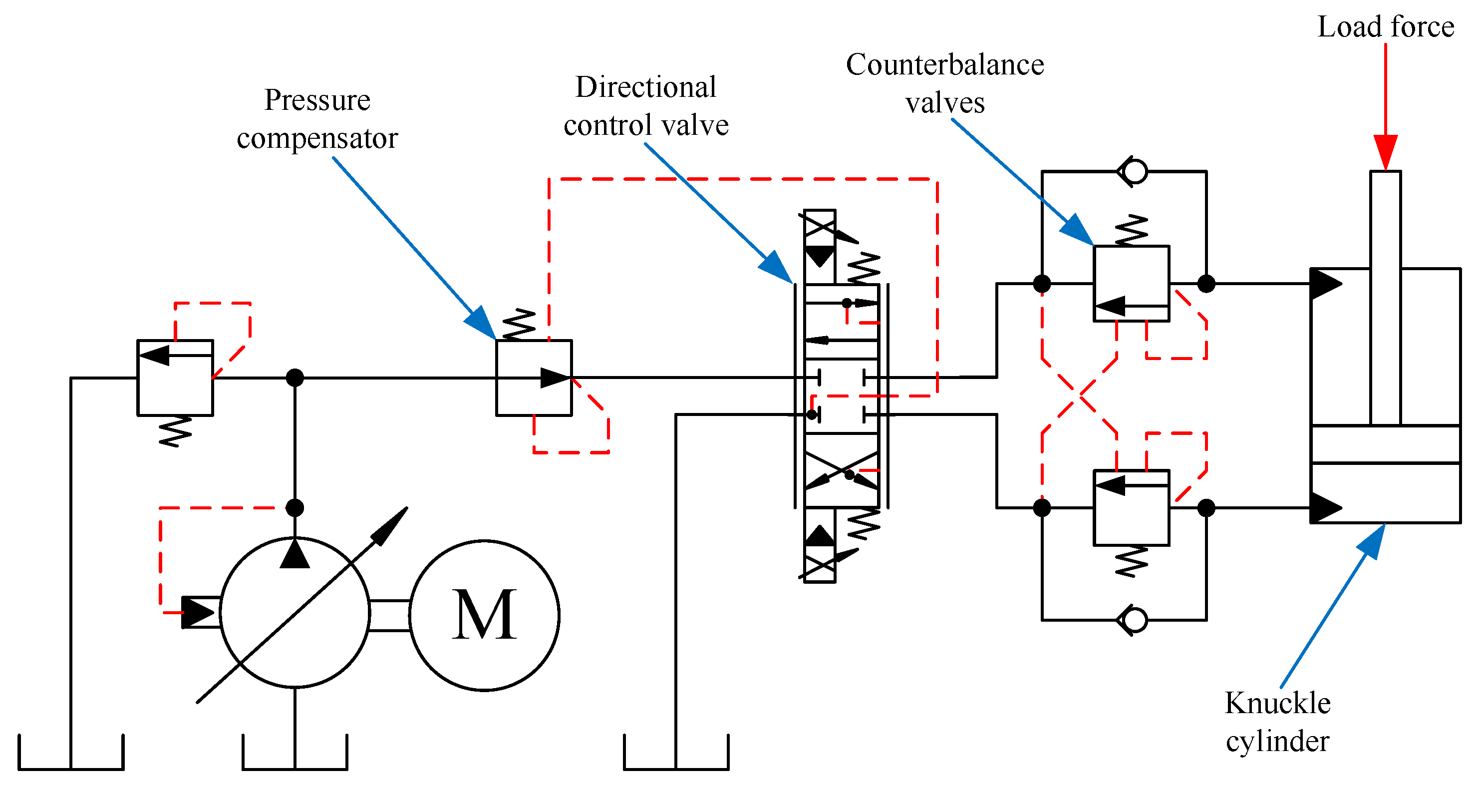
Figure 2.
Hydraulic system of the knuckle cylinder.
Figure 2.
Hydraulic system of the knuckle cylinder.
Figure 3.
Control strategy with the novel deflection compensators highlighted in light blue.
Figure 3.
Control strategy with the novel deflection compensators highlighted in light blue.
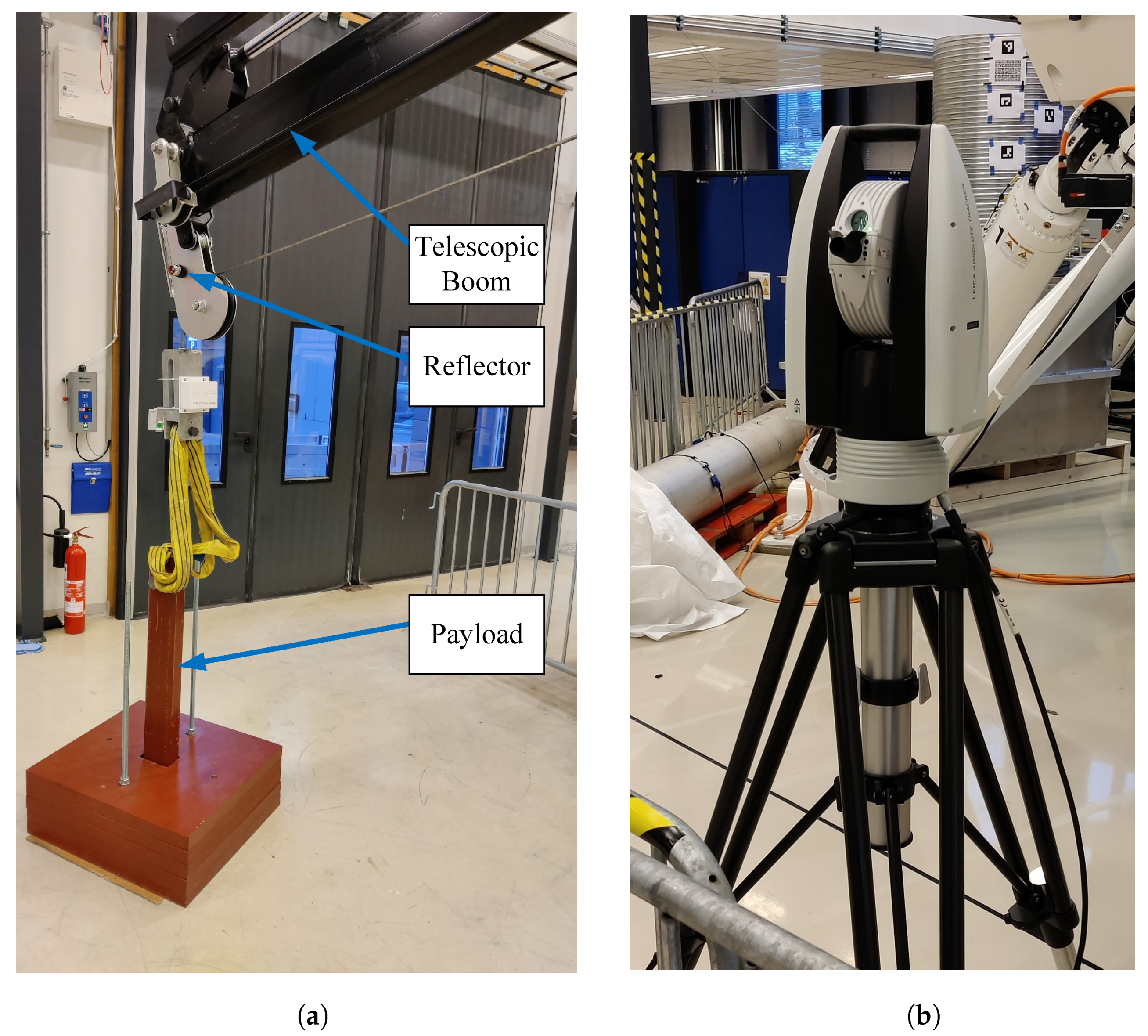
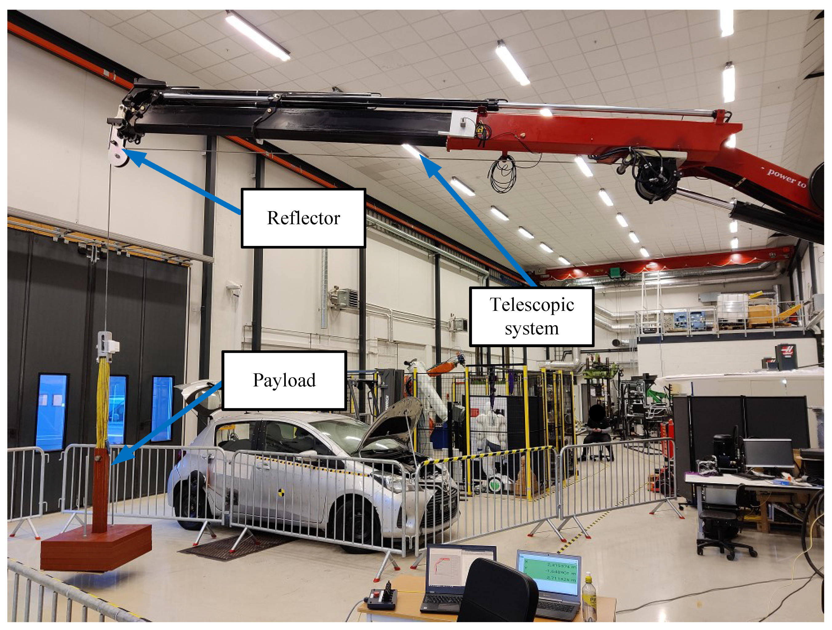
Figure 4.
Experimental setup in the lab. The laser tracker measures the crane tip position using the attached reflector. (a) Crane tip showing the telescopic boom, reflector, and payload, (b) Leica Absolute Tracker AT960.
Figure 4.
Experimental setup in the lab. The laser tracker measures the crane tip position using the attached reflector. (a) Crane tip showing the telescopic boom, reflector, and payload, (b) Leica Absolute Tracker AT960.
Figure 5.
Crane tip position in -plane with and without load from laboratory measurements. Crane position illustrated in black with its three degrees of freedom.
Figure 5.
Crane tip position in -plane with and without load from laboratory measurements. Crane position illustrated in black with its three degrees of freedom.
Figure 6.
Crane geometry showing joint angles, lifting radius R, telescopic length , and crane tip position.
Figure 6.
Crane geometry showing joint angles, lifting radius R, telescopic length , and crane tip position.
Figure 7.
Crane geometry used with Denavit–Hartenberg parameters.
Figure 7.
Crane geometry used with Denavit–Hartenberg parameters.
Figure 8.
Illustration of the main joint actuator kinematics.
Figure 8.
Illustration of the main joint actuator kinematics.
Figure 9.
Curve fit for inverse actuator kinematics. (a) Curve fit for main cylinder, (b) Curve fit for knuckle cylinder.
Figure 9.
Curve fit for inverse actuator kinematics. (a) Curve fit for main cylinder, (b) Curve fit for knuckle cylinder.
Figure 10.
Illustration of a single node.
Figure 10.
Illustration of a single node.
Figure 11.
Overview of the neural network.
Figure 11.
Overview of the neural network.
Figure 12.
Predicted deflection in x-direction . Black dots show measured data from the laboratory. (a) Predicted with = 2.973 m. (b) Predicted with = 4.567 m.
Figure 12.
Predicted deflection in x-direction . Black dots show measured data from the laboratory. (a) Predicted with = 2.973 m. (b) Predicted with = 4.567 m.
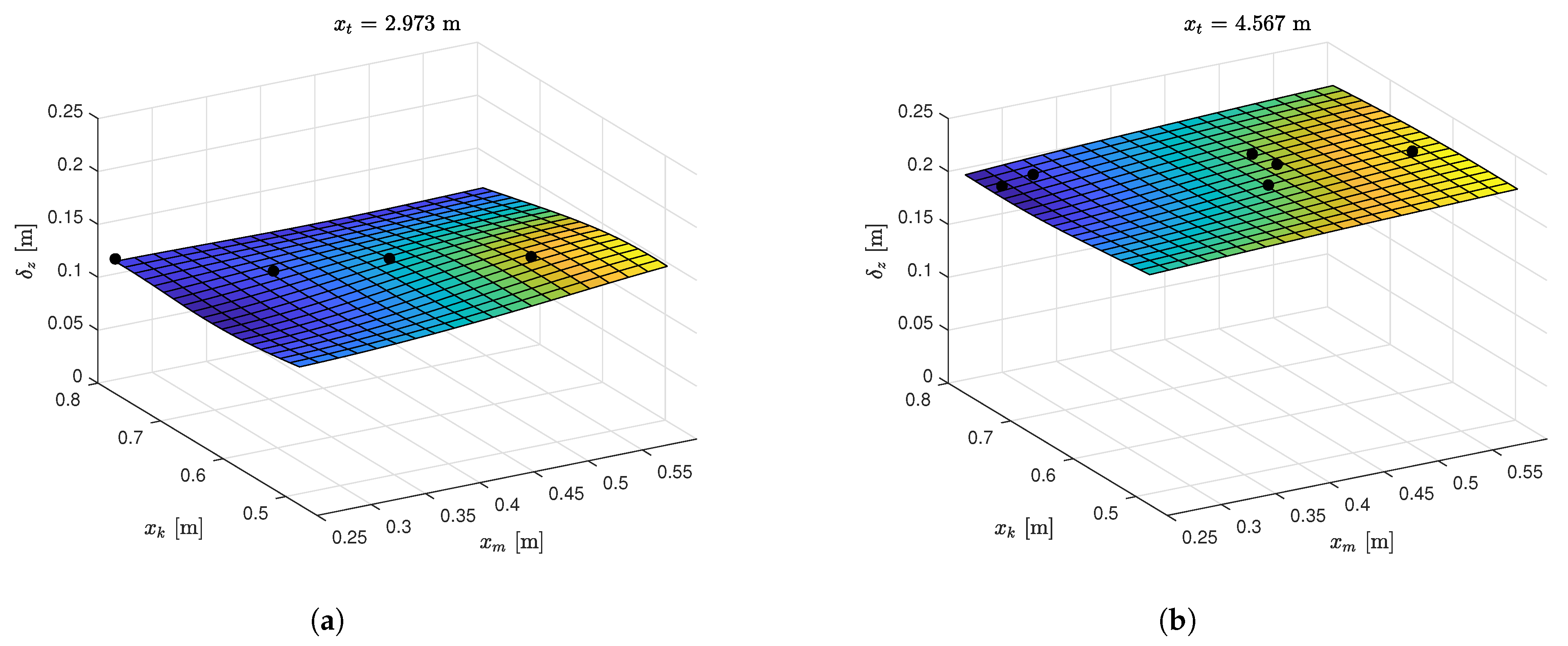
Figure 13.
Predicted deflection in z-direction . Black dots show measured data from the laboratory. (a) Predicted with = 2.973 m. (b) Predicted with = 4.567 m.
Figure 13.
Predicted deflection in z-direction . Black dots show measured data from the laboratory. (a) Predicted with = 2.973 m. (b) Predicted with = 4.567 m.
Figure 14.
Block diagram of the static deflection compensator.
Figure 14.
Block diagram of the static deflection compensator.
Figure 15.
Crane tip oscillations from laboratory.
Figure 15.
Crane tip oscillations from laboratory.
Figure 16.
Estimated crane natural frequency.
Figure 16.
Estimated crane natural frequency.
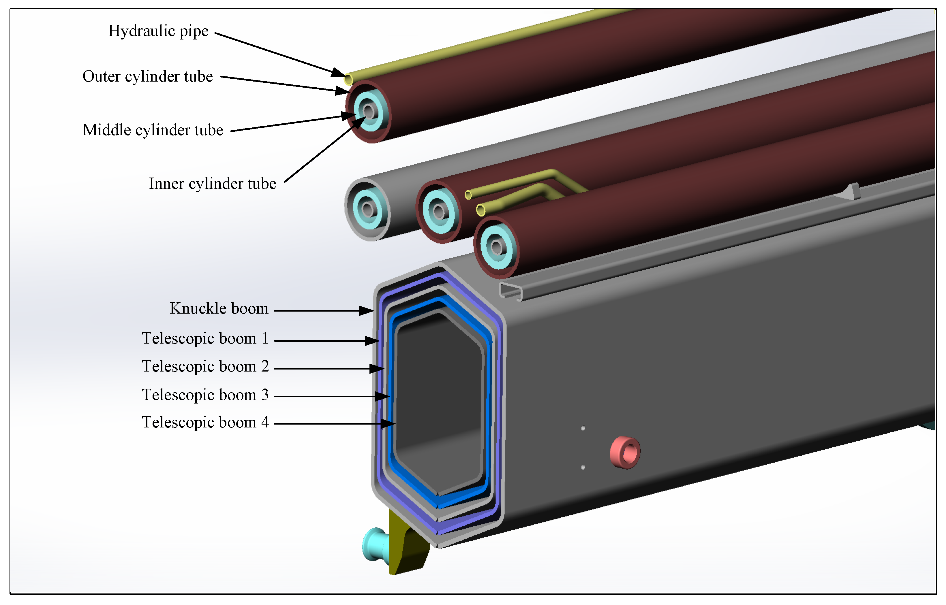
Figure 17.
Section view of the telescopic system, from CAD model.
Figure 17.
Section view of the telescopic system, from CAD model.
Figure 18.
Illustration of a telescopic cylinder.
Figure 18.
Illustration of a telescopic cylinder.
Figure 19.
Hydraulic system for the telescopic cylinders.
Figure 19.
Hydraulic system for the telescopic cylinders.
Figure 20.
Flows in the telescopic circuit. (a) Flows in the telescopic circuit during out-stroke motion. (b) Flows in the telescopic circuit during in-stroke motion.
Figure 20.
Flows in the telescopic circuit. (a) Flows in the telescopic circuit during out-stroke motion. (b) Flows in the telescopic circuit during in-stroke motion.
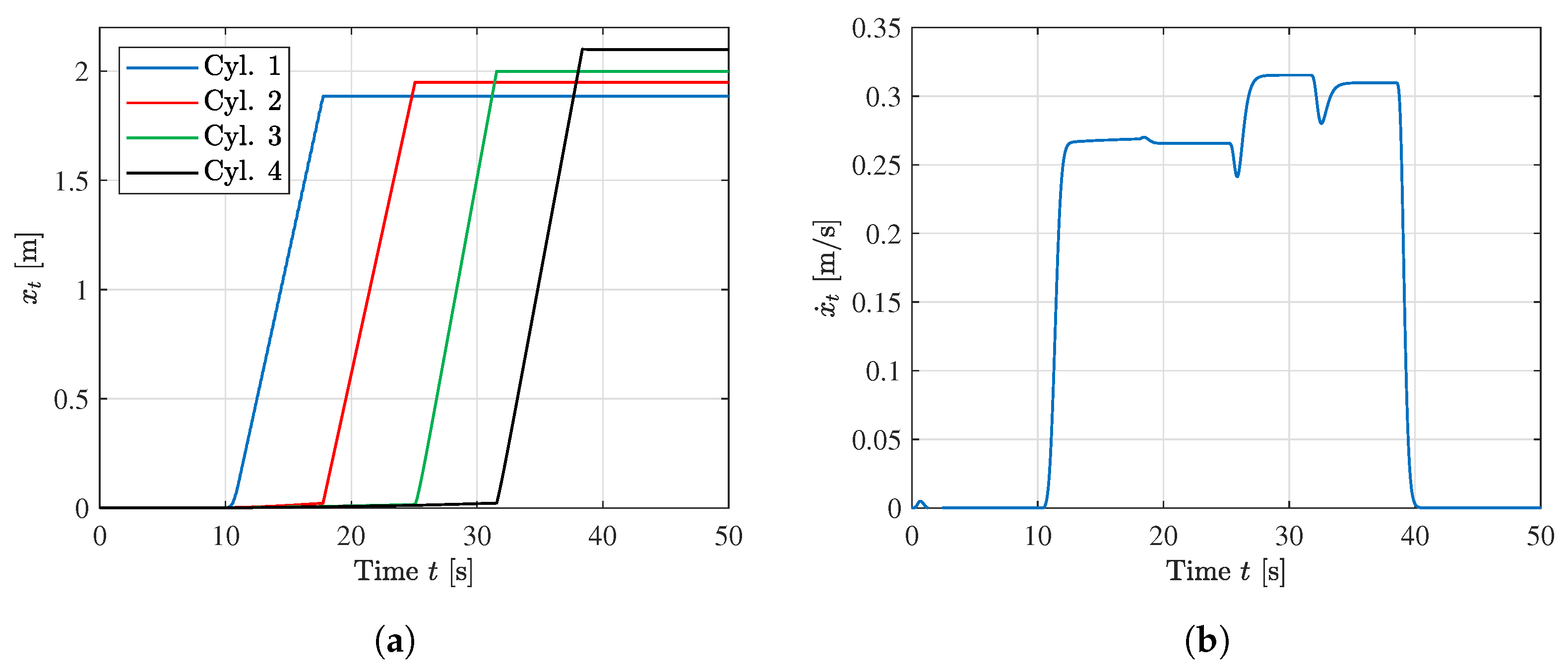
Figure 21.
Motion sequence and velocity of the telescopic cylinders. (a) Position of each telescopic cylinder. (b) Velocity of the full telescopic system.
Figure 21.
Motion sequence and velocity of the telescopic cylinders. (a) Position of each telescopic cylinder. (b) Velocity of the full telescopic system.
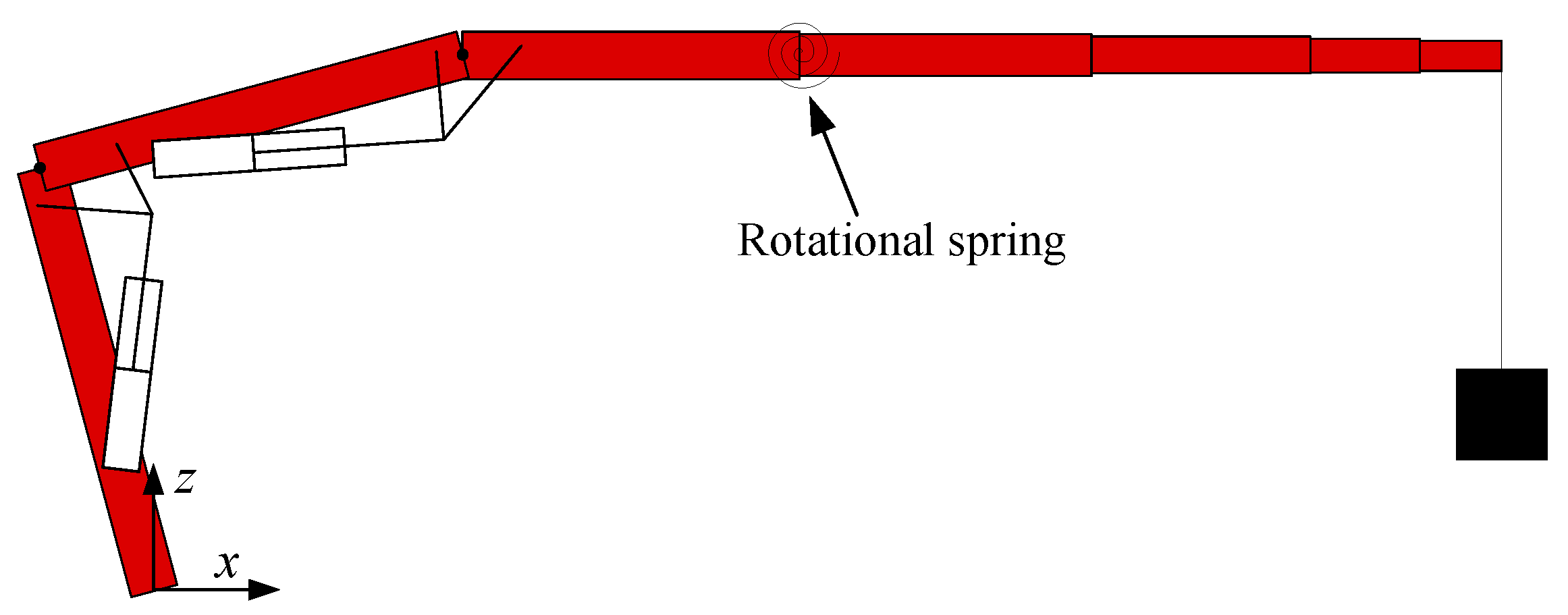
Figure 22.
Illustration of the simplified flexible model.
Figure 22.
Illustration of the simplified flexible model.
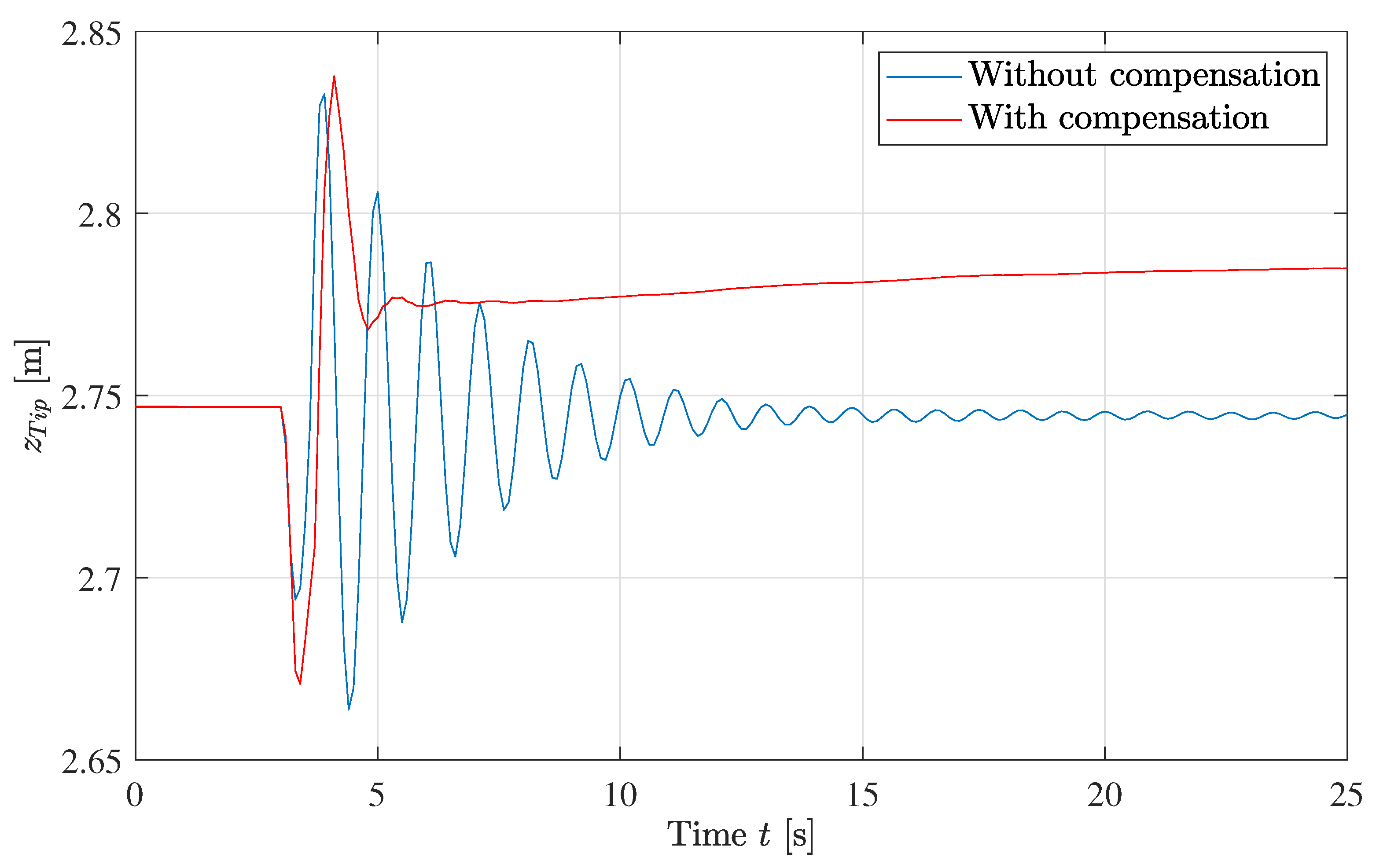
Figure 23.
The vertical coordinate of the crane tip, , is plotted as a function of time for three different conditions.
Figure 23.
The vertical coordinate of the crane tip, , is plotted as a function of time for three different conditions.
Figure 24.
Effects of the static and dynamic deflection compensator. (a) Change in cylinder position reference from the static deflection compensator, (b) control signal from the dynamic deflection compensator , and motion controller .
Figure 24.
Effects of the static and dynamic deflection compensator. (a) Change in cylinder position reference from the static deflection compensator, (b) control signal from the dynamic deflection compensator , and motion controller .
Figure 25.
Experimental setup in the laboratory, showing the crane with a hanging load.
Figure 25.
Experimental setup in the laboratory, showing the crane with a hanging load.
Figure 26.
Crane tip position in the -plane during motion in laboratory.
Figure 26.
Crane tip position in the -plane during motion in laboratory.
Figure 27.
The vertical coordinate of the crane tip, , plotted as a function of time during motion in laboratory.
Figure 27.
The vertical coordinate of the crane tip, , plotted as a function of time during motion in laboratory.
Figure 28.
Effects of the static and dynamic deflection compensator in laboratory. (a) Change in cylinder position reference from the static deflection compensator. (b) Control signal from the dynamic deflection compensator.
Figure 28.
Effects of the static and dynamic deflection compensator in laboratory. (a) Change in cylinder position reference from the static deflection compensator. (b) Control signal from the dynamic deflection compensator.
Figure 29.
Load impulse test with only dynamic compensator activated.
Figure 29.
Load impulse test with only dynamic compensator activated.
| Name | Length [m] |
|---|
| |
| |
| |
| |
| |
| |
Table 2.
Denavit–Hartenberg parameters.
Table 2.
Denavit–Hartenberg parameters.
| | | |
|---|
| 0 | | | |
| 0 | 0 | |
| 0 | | | |
| 0 | 0 | |
| 0 | | | 0 |
| 0 | 0 | | 0 |
Table 3.
Lengths of the parts in the main linkage.
Table 3.
Lengths of the parts in the main linkage.
| Name | Length [m] |
|---|
| |
| |
| |
| |
| |
| |
Table 4.
Curve-fitting coefficients for inverse actuator kinematics.
Table 4.
Curve-fitting coefficients for inverse actuator kinematics.
| Coefficient | Main | Knuckle |
|---|
| | |
| | |
| | |
| | |
| | |
| | |
| | |
| | |
| | |
| | |
Table 5.
Telescopic cylinder data, in [mm].
Table 5.
Telescopic cylinder data, in [mm].
| | | | | | | | h |
|---|
| Cylinder 1 | 80 | 70 | 55 | 35 | 20 | 15 | 1885 |
| Cylinder 2 | 80 | 70 | 55 | 35 | 20 | 15 | 1950 |
| Cylinder 3 | 80 | 70 | 50 | 34 | 20 | 15 | 2000 |
| Cylinder 4 | 80 | 70 | 50 | 34 | 20 | 15 | 2100 |
Table 6.
Identified deadband for the actuators.
Table 6.
Identified deadband for the actuators.
| Actuator | Out, | In, |
|---|
| Main | 0.24 | −0.22 |
| Knuckle | 0.20 | −0.31 |
| Telescope | 0.33 | −0.33 |
Table 7.
Parameters used in laboratory.
Table 7.
Parameters used in laboratory.
| Description | Name | Value |
|---|
| Main feedback | | 15 m−1 |
| Main out-stroke feedforward | | s/m |
| Main in-stroke feedforward | | s/m |
| Knuckle feedback | | 20 m−1 |
| Knuckle out-stroke feedforward | | s/m |
| Knuckle in-stroke feedforward | | s/m |
| Telescope feedback | | 2 m−1 |
| Telescope out-stroke feedforward | | s/m |
| Telescope in-stroke feedforward | | s/m |
| Pressure feedback gain | | 0.02 bar−1 |


