A Novel, Oriented to Graphs Model of Robot Arm Dynamics

Abstract

Robotics is an interdisciplinary field and there exist several well-known approaches to represent the dynamics model of a robot arm. The robot arm is an open kinematic chain of links connected through rotational and translational joints. In the general case, it is very difficult to obtain explicit expressions for the forces and the torques in the equations where the driving torques of the actuators produce desired motion of the gripper. The robot arm control depends significantly on the accuracy of the dynamic model. In the existing literature, the complexity of the dynamic model is reduced by linearization techniques or techniques like machine learning for the identification of unmodelled dynamics. This paper proposes a novel approach for deriving the equations of motion and the actuator torques of a robot arm with an arbitrary number of joints. The proposed approach for obtaining the dynamic model in closed form employs graph theory and the orthogonality principle, a powerful concept that serves as a generalization for the law of conservation of energy. The application of this approach is demonstrated using a 3D-printed planar robot arm with three degrees of freedom. Computer experiments for this robot are executed to validate the dynamic characteristics of the mathematical model of motion obtained by the application of the proposed approach. The results from the experiments are visualized and discussed in detail.

1. Introduction

There exist several different approaches for modeling the motion of robot arms in the existing literature. Most frequently, the kinematic aspects of motion are expressed by Denavit–Hartenberg parameters, Euler angles, or normalized quaternions [1]. It is usually difficult to integrate these models with Newton-Euler, Lagrange and Hamilton methods employed to represent the dynamic model [2,3]. This is especially true for robot arms with redundant degrees of freedom, where the redundancy allows improving the quality of motion by introducing optimization criteria. In the existing literature, these criteria are defined on the level of kinematics or dynamics. Time optimization, manipulability, or obstacle avoidance are some of the typical criteria for optimal path planning at the kinematical level [4,5,6]. Singularity avoidance is another popular way to exploit redundant degrees of freedom in executing a given task [7,8,9]. Criteria related to energy saving represent a special interest if the level of dynamics is concerned [10,11].

The accuracy of motion control of a physical robot arm strongly depends on the completeness of the model of dynamics. The dynamic system model describes the relationship between the forces and torques applied to the robot arm on the one hand and the resulting robot arm motion in joint space or workspace coordinates on the other hand. The equations of motion serve to solve the forward and the inverse dynamic problems, respectively [12,13]. Given the motion in the joint space or workspace, these equations determine the driving torques of the actuators in the joints or the forces of the gripper. In the inverse problem, the motion in the joint space or workspace is computed knowing the driving torques in the joints. In the existing literature, there are several approaches to obtain the dynamics equations of motion.

The Lagrangian formulation is one of the most frequently used approaches to describe mechanical phenomena. Apparently, this approach does not allow to consider the reaction forces, while it is essential to know these forces at the stage of design in order to select, for instance, the optimal bearing in the joints. A related research paper [14] follows the same approach and emphasizes the computation of differential algebraic equations of the dynamics model, where the reaction forces are not considered. Although the electrical phenomena are out of the scope of this paper, for completeness, note that there are attempts to complement the Lagrangian function with terms reflecting electrical characteristics in terms of electro-mechanical analogies [15]. It appears, however, that this is impossible in the analysis of case studies involving sliding contacts and volume currents. In such cases, the Lagrangian formulation is not applicable because there are no suitable electro-mechanical analogs.

The limitations in the application of the Lagrangian formulation can be resolved provided the dynamic system model is built on the conservation of energy law. Unlike the Lagrangian formulation, the law of conservation of energy allows extending the modeling process so that it includes objects pertinent to electrical and magnetic phenomena, as well as considering the energy flow between objects intrinsic to robot arm devices [16]. Therefore, this paper employs the law of conservation of energy rather than the Lagrangian formulation to develop and obtain the dynamic model of a robot arm.

The equations, describing the dynamic model, are nonlinear and one of the most widely used approaches is to simplify these equations in terms of numerical approximation [17]. Other computational techniques use Iterative learning control for dealing with unmodelled dynamics [18], or deep learning for the estimation of dynamics parameters [19]. These approaches are usually implemented in software tools for processing the kinematic and dynamic characteristics of the robot arm design obtained with advanced CAD systems like SolidWorks. The 3D CAD model of the robot arm supports nowadays both its manufacturing process, as well as the analysis and simulation of its motion in a workspace. For example, the parameters of the assembly model like mass, inertia moments, geometrical parameters of the links, can be imported in the integrated environment of MATLAB, Simscape and Simulink software products. Thus, the powerful functionalities of these products are utilized for computing and simulating the behavior of a robot arm dynamic model. Several research papers investigate the application of such CAD-based methodologies for developing the dynamic model of a robot. These papers consider, however, special cases of robot devices, where the results are restricted to deriving the equations of kinematics [20] or the built-in functionalities of the software packages don’t allow to consider in explicit form important parameters of the dynamic model, such as drive torques and forces [21]. Apparently, the CAD model can assist in extracting the basic characteristics of kinematics and dynamics, however, the complex nonlinear relationships inherent to a robot arm cannot be obtained from a CAD model in a fully automatic way. At present, the dynamic system model can be obtained in closed-form only in some particular cases [22]. In the general case, however, the analytical representation of the complete equations of motion remains a challenge that the model proposed in this paper aims to resolve.

The objective of this paper is to propose an approach for modeling, in closed form, the dynamics of robot arms with an open kinematic chain, having rotational or translational joints of the fifth class. The proposed model of the dynamics borrows ideas from the paper of Tellegen [23] where graphs, in combination with terms of “through” (current) and “across” (voltage) variables, are introduced to represent electrical networks in a practicable, convenient way. Further on, these ideas are elaborated in the research works of Blackwell [24] and Andrews [25]. Blackwell considers merely electro-mechanical systems with simple mechanical components. Andrews introduces the orthogonality principle for the first time but only in relation to models of dynamics dealing with mass points. Later on, graph theory is introduced to design interconnected systems of multi-bodies in related research papers [26,27]. Thus, the orthogonality principle became applicable for industrial robots [28,29]. A detailed description of the proposed approach in such cases is presented here. Without loss of generality, the non-conservative friction effects are left out of scope in this study, although the law of conservation of energy allows taking them into account in the proposed dynamic model by means of the same approach. The study of these effects represents a subject for separate research work and for simplicity of presentation, these effects are not considered here. Finally, the paper demonstrates how to apply this approach in the case of a proprietary physical model of a robot arm. Results from computer experiments with the obtained explicit equations of motion in this real-life case study are provided to validate the correctness of the model of dynamics.

The paper is structured in four sections. The following section describes the development of the kinematics and dynamics model of a robot arm. The results from computer experiments are visualized and discussed in Section 3. Section 4 provides a discussion on the advantages and disadvantages of this approach in view of its application in the field of industrial robotics. This final section summarizes the main results of the paper.

2. Materials and Methods

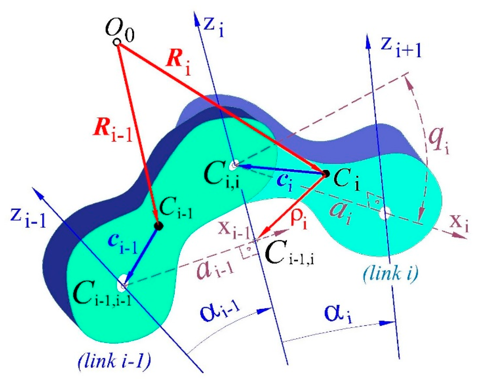
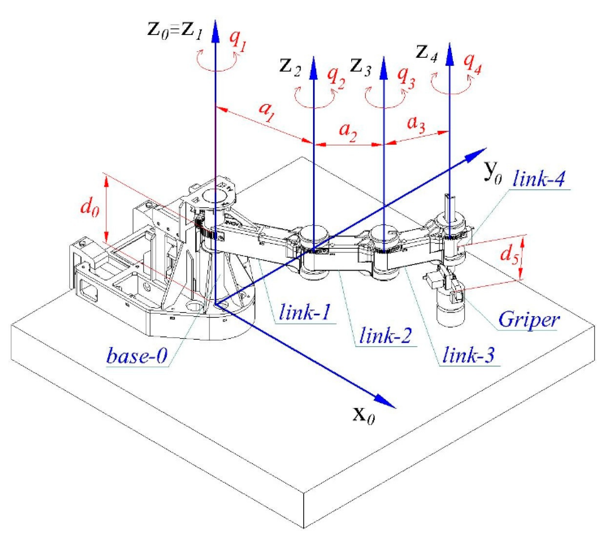
This section provides a detailed description of the proposed uniform approach for developing a mathematical model of the robot arm dynamics. The graph theory allows the application of the orthogonality principle in deriving the dynamic’s equations of motion of the robot arm. For clarity, a procedure for applying the proposed approach in the general case is here provided. The implementation of the procedure is demonstrated in a real-life case study, where the actuator torques are computed from the obtained equations in executing a given robot arm motion.

2.1. Kinematics

In this paper, we consider a robot arm with an open kinematic chain with $n$ DoF. The links of the robot arm are $n+1$ rigid bodies (including the base) with translational or rotational joints of the fifth class. The vector of the generalized coordinates $q={({\mathrm{q}}_1,{\mathrm{q}}_2,\dots .,{\mathrm{q}}_{\mathrm{n}})}^{\mathrm{T}}$ is used to describe the forward kinematics in the workspace $\mathrm{W}$ in terms of the linear and angular position of the gripper of the robot arm. In practice, the dimension of $\mathrm{W}$ is equal to the number of parameters required to define the work task executed by the robot arm. For clarity, assume the dimension of $\mathrm{W}$ is $m$. Special interest represents the case $n>m$ when the robot arm has redundant DoF.

Forward kinematics is expressed by means of Denavit–Hartenberg notation as follows (Figure 1). A coordinate system $O_i{\mathit{x}}_i{\mathit{y}}_i{\mathit{x}}_i$ with unit vectors ${\mathit{e}}_1^{\left(i\right)}, {\mathit{e}}_2^{\left(i\right)}, {\mathit{e}}_3^{\left(i\right)}$ is fixed in each link $i, i=0, 1, 2, \dots ,n$, where the coordinate system $O_0{\mathit{x}}_0{\mathit{y}}_0{\mathit{z}}_0$ is attached to the base. The axis ${\mathit{z}}_i$ coincides with the axis of relative motion of link $i+1$ with respect to link $i$. For convenience, the axis ${\mathit{z}}_0$ is chosen to coincide with ${\mathit{z}}_1$ and $O_0\equiv O_1$. Similarly, the axis ${\mathit{z}}_n$ is appropriately chosen to represent the axis of relative motion of the gripper. The axis ${\mathit{x}}_i$ is orthogonal to both ${\mathit{z}}_{i-1}$ and ${\mathit{z}}_i$,whereby ${\mathit{x}}_i$ is oriented towards ${\mathit{z}}_i$. The axis ${\mathit{y}}_i$ complements $O_i{\mathit{x}}_i{\mathit{y}}_i{\mathit{z}}_i$ to right-handed coordinate system. On each axis ${\mathit{z}}_i$ two points $C_{i,i}$ and $C_{i-1,i}$ are chosen, where the first of them is fixed in the link $i$ and the second in link $i-1$.

Definition 1.

The point $C_{i-1,i}$is referred to as contact point of link$i-1$with joint$i$.

For convenience, select point $C_{i,i}\equiv O_i$ and point $C_{i-1,i}$ as the intersection point of axes ${\mathit{x}}_{i-1}$ and ${\mathit{z}}_i, i=1, 2, \dots n.$ Without loss of generality, assume $C_{0,1}$ coincides with the origin $O_0$ of the base coordinate system. Let the distance between two adjacent coordinate systems be represented by vector $d_i=C_{i-1,i} C_{i,i}$ along ${\mathit{z}}_i$. Denote by ${\alpha }_i$ and $a_i$ the angular displacement between axes ${\mathit{z}}_i$ and ${\mathit{z}}_{i-1}$ and the vector $a_i=C_{i-1,i-1} C_{i-1,i}$. measured along axis ${\mathit{x}}_i$. The generalized coordinates ${\mathrm{q}}_{\mathrm{i}}$ represent the relative translation or relative rotation along ${\mathit{z}}_i$ in case joint $i$ is translational or rotational joint correspondingly. For convenience, the motion of the robot arm links with respect to $O_0{\mathit{x}}_0{\mathit{y}}_0{\mathit{z}}_0$ is considered in the following sections in terms of coordinate systems $C_i{\mathit{x}}_i{\mathit{y}}_i{\mathit{z}}_i, i=1, 2, \dots ,n$ obtained by translating $O_i{\mathit{x}}_i{\mathit{y}}_i{\mathit{z}}_i$ in the mass centers $C_i, i=1, 2, \dots ,n$ by vector $c_i=C_i C_{i,i}$ (Figure 1). Then, the absolute linear position of link $i$ is given by the respective vector $R_i\left(q\right)$. Further on, the locations ${\rho }_i$ of the contact points $C_{i-1,i}$, $i=1, 2, \dots ,n$ in $C_i{\mathit{x}}_i{\mathit{y}}_i{\mathit{z}}_i$ are used to represent important constructs in the proposed dynamics model.

2.2. Dynamics

In this section, the robot arm model of dynamics is built making use of the orthogonality principle [24,27]. This principle is strongly related to energy flow and energy potential. The theory of graphs offers a convenient technique to manage effectively these basic characteristics of the energy conservation law. In the related literature [24,25], the energy flow and energy potential are expressed in terms of so-called “through” and “across” variables in accordance with the following definitions.

Definition 2.

Across variables are the variables representing the energy potential characteristics.

Definition 3.

Through variables are the variables representing the energy flow characteristics.

The linear and angular velocities as well as the radius vectors ${\mathbf{\rho }}_i i=1, 2, \dots ,n$ of the contact points and the radius vectors $R_i$ in Figure 1 are examples of across variables. On the other side, forces and torques are typical representatives of through variables in the existing literature [24]. Pairs of across and through variables provide means to describe translational and rotational motion correspondingly.

In this paper we employ a graph, referred to as energy graph, to model the energy flow and energy potential.

Definition 4.

Energy graph is the graph where each edge is associated with a pair of across and through variables and the vertices are the mass centers $C_i$and the contact points$C_{i-1,i}, i=1, 2, \dots ,n$. The root vertex of the energy graph is the origin$O_0$of the base coordinate system$O_0{\mathit{x}}_0{\mathit{y}}_0{\mathit{z}}_0$.

The thus introduced energy graph is employed in the following subsections to outline a procedure for deriving the differential equation of dynamics.

2.2.1. Energy Graph Associated with Robot Arm

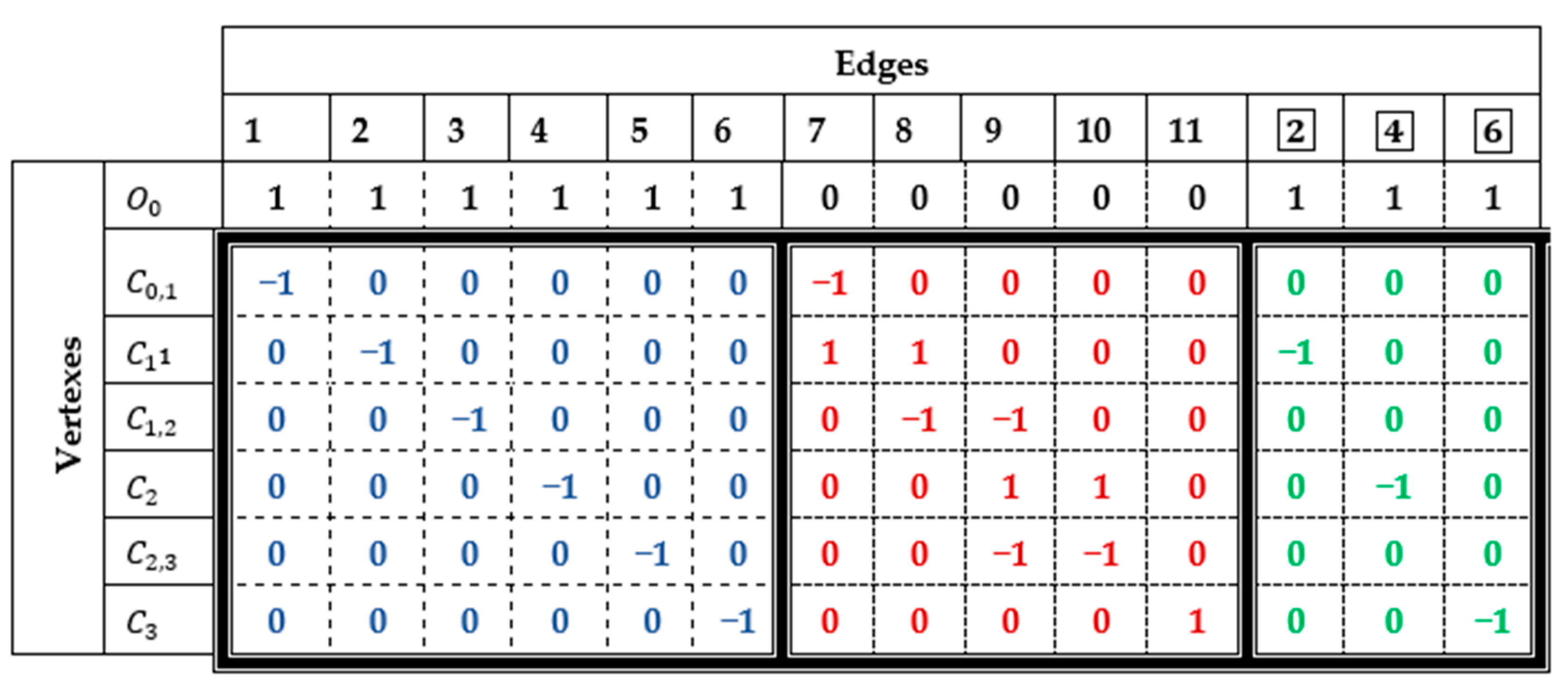
In the following sections, we consider the energy graph as the union of two nonintersecting graphs ${\mathrm{G}}_{\mathrm{p}}$ and ${\mathrm{G}}_{\mathrm{r}}$. The edges in the energy graph with across variables related to linear displacement are part of ${\mathrm{G}}_{\mathrm{p}}$ and the edges with across variables dealing with angular displacement build-up ${\mathrm{G}}_{\mathrm{r}}$. For example, the absolute linear velocity $\mathit{v}$ and force $\mathit{F}$ applied in the mass center $C$ of a free rigid body as well as the absolute angular velocity $\mathit{\omega }$ and torque $\mathit{T}$ with respect to its mass center represent such pairs (Figure 2) in the energy graph. Accordingly, the first pair is an edge in ${\mathrm{G}}_{\mathrm{p}}$ and the second pair is an edge in ${\mathrm{G}}_{\mathrm{r}}.$ Note that both edges connect the origin of the base coordinate system with the mass center.

Consider now the energy graph in the general case of a robot arm with an open kinematic chain. Both ${\mathrm{G}}_{\mathrm{p}}$ and ${\mathrm{G}}_{\mathrm{r}}$ have the same topological structure shown in Figure 3. Similarly to the case of a free rigid body ${\mathrm{G}}_{\mathrm{p}}$ and ${\mathrm{G}}_{\mathrm{r}}$ have edges that connect the origin of $O_0{\mathit{x}}_0{\mathit{y}}_0{\mathit{z}}_0$. with the respective mass center $C_i$ of the bodies in the kinematic chain. These edges are shown in black color in Figure 3.

The links of the robot arm are connected with joints and this requires considering the reactions in the joints by introducing in the topological structure vertices representing the contact points $C_{i-1,i}, i=1, 2, \dots n$ of the links in the respective joints.

Therefore, we add edges in ${\mathrm{G}}_{\mathrm{p}}$ and ${\mathrm{G}}_{\mathrm{r}}$ with pairs of across and through variables related to the reactions in the joints. These edges are shown in red color in Figure 3. Apparently, graphs ${\mathrm{G}}_{\mathrm{p}}$ and ${\mathrm{G}}_{\mathrm{r}}$ are oriented graphs with different pairs of across and through variables attached to their edges. Each graph ${\mathrm{G}}_{\mathrm{p}}$ and ${\mathrm{G}}_{\mathrm{r}}$ has $2n+1$ vertices (corresponding to the number of links including the base coordinate system) and $5n-1$ edges. Part of the vertices are the mass centers $C_i, i=1, 2, \dots , n$ of robot links and the remaining are the contact points $C_{i-1,i}$. All the vertices are connected with the origin of the base coordinate system.

Definition 5.

A cycle in a graph is the set of edges connecting two different vertices of the graph.

According to this definition the edges of ${\mathrm{G}}_{\mathrm{p}}$ and ${\mathrm{G}}_{\mathrm{r}}$ can be considered to belong to two separate sets, namely, branches and chords.

Definition 6.

An edge is referred to as a branch when this edge does not belong to a cycle.

Definition 7.

An edge is referred to as a chord when this edge connects two vertices belonging to a branch.

Apparently, a chord introduces cycles in the topological structure of the energy graph. Therefore, the cycle orientation is equal to the orientation of the chord generating the cycle as shown with a dashed line in pink color in Figure 3. The edges denoted by $1, 2, \dots , n$ in Figure 3 refer to pairs of across and through variables interpreting a resulting force (graph ${\mathrm{G}}_{\mathrm{p}}$) or a resulting torque (graph ${\mathrm{G}}_{\mathrm{r}}$) are considered as branches and these are denoted in black color in Figure 3. Through variables referring to external forces and torques are represented in terms of chords denoted by numbers framed in green color. Each of these numbers is related to the number used to denote the branch pointing to the mass center where the corresponding external force is applied to. In case the external forces applied to a mass center are represented by their resultant force then these numbers are the same. For example, the external forces applied in the mass centers are represented in Figure 3 by their resultant force. Therefore, the through variables of these resultant forces are indexed by the same numbers as the branches pointing to the respective mass center. For example, both the through variable (denoted inside a green frame) of the resultant force applied to the mass center $C_1$ and the branch number (denoted in black) is equal to 2. Without loss of generality, the resultant forces include only the gravity forces applied to the mass centers $C_i, i=1, 2, \dots , n$ are taken into consideration. In the general case, each external force applied to $C_i$ can be introduced by adding a separate through variable, where its number in the green box must be indexed in relation to the branch number $2i,, i=1, 2, \dots , n.$ Note that these variables can be used to represent torques induced by external forces as well. Through variables referring to reactions like the resultant of the reaction forces applied in the joints are represented also by the chords with numbers displayed in red color in Figure 3.

Consider closer graph ${\mathrm{G}}_{\mathrm{p}}$. The $n$ edges in ${\mathrm{G}}_{\mathrm{p}}$ that are numbered in green frames represent the variables related to external forces. For simplicity, here only the gravity force is considered. The branches start from vertex $O_0$ to $C_i$ and $C_{i-1,i}$,$i=1, 2, \dots , n$, while the remaining edges are chords.

The following through variables are represented in the graph ${\mathrm{G}}_{\mathrm{p}}$ having the topological structure shown in Figure 3:

• The D’Alembert forces $F_{2i}^d, i=1, 2, \dots , n$, associated with the edges numbered in black and denoted by $2i, i=1, 2, \dots , n$.
• The forces $F_{2i-1}, i=1, 2, \dots , n$, applied in the points $C_{i-1,i}$ with the edges numbered in blue and denoted by $2i$−1. Note, that only $F_1\ne 0$ because the first body is linked with the base coordinate system.
• The resultant of the external forces $F_{2i}, i=1, 2, \dots , n$, applied in the mass centers are represented by edges numbered $2i,, i=1, 2, \dots , n$ in green frame.
• The forces $F_i^c, i=2n+1, \dots , 4n-1$ of interaction between the adjacent bodies are represented by edges numbered in red and denoted by $i=2n+1, \dots , 4n-1$.

The across variables associated with the graph ${\mathrm{G}}_{\mathrm{p}}$ are:

• The radius-vectors of the mass-centers $C_i$ and the points $C_{i-1,i}$ starting from $O_0$.
• The local radius-vectors of $C_{i-1,i}$ relative to the mass centers $C_i$ for the remaining edges.

The edges with numbers from 1 to $2n$ are chosen as branches [25,26] and all the other edges are chords. The same enumeration style is used for the angular velocities related to the edges of the graph ${\mathrm{G}}_{\mathrm{r}}$.

Graph ${\mathrm{G}}_{\mathrm{r}}$ has the same topological structure as ${\mathrm{G}}_{\mathrm{p}}$ where the through variables have the following interpretation.

• The D’Alembert torques $T_{2i}^d, i=1, 2, \dots , n$, associated with the edges numbered in black and denoted by $2i, i=1, 2, \dots , n$.
• The torques $T_{2i-1}, i=1, 2, \dots , n$, acting on the points $C_{i,j}$ associated with the edges numbered in blue and denoted by $2i$−1. Note, that only $T_1\ne 0$ because the first body is linked with the base coordinate system.
• The resultant of the external torques $T_{\left(2i\right)}, i=1, 2, \dots , n$ applied in the joint axes s are represented by edges numbered in the green frame by $2i,, i=1, 2, \dots , n$.
• The torques $T_i^c, i=2n+1, \dots , 4n-1$ of interaction between the connected bodies are represented by edges numbered in red and denoted by $i=2n+1, \dots , 4n-1$.

The across variables associated with graph ${\mathrm{G}}_r$ are determined as follows. For each of the edges starting from $O_0$ the across variable is the absolute angular velocity of the link matching the vertex the respective edge is directed to. These across variables are denoted by $X_b^r.$ The vertices $C_{i-1,i}$ in this graph correspond to contact points $C_{i-1,i}$ belonging to links with number $i-1$ in Figure 3. Thus, the “angular” velocity of such vertex is assumed to coincide with the angular velocity of the respective link. The across variables for chords starting from the mass centers $C_i$ describe relative angular velocities and those with even numbers are zeroes according to the assumption for the contact points $C_{i-1,i}$. These across variables are denoted by $X_c^r$.

2.2.2. Cut-Set and Circuit Equations

The energy conservation law cannot be proved but is always under verification. One of its formulations states that the energy is not created or destroyed; it can only be transformed from one kind to another. This way our system can accept energy, and transform it according to its functioning, and return back the remainder after that. In this paper, the system is interpreted by a graph whose edges are associated with pairs of across and through variables. The energy conservation law is known in the area of mechanics as the orthogonality principle. This principle can be formulated in terms borrowed from graph theory as “The sum over all the edges of the scalar products of the through and the across variables associated with each edge of the graph must be zero”.

The oriented graph with the topological structure shown in Figure 3 has $\mathsf{\nu }=2n+1$ vertices and $\sigma =5n-1$ edges. Then, the branches are $\mathsf{\nu }-1=2n$ and the chords are $\sigma -\left(\mathsf{\nu }-1\right)=3n-1$. After the elimination of the across variables it follows that (1):

$${\displaystyle \sum }_{j=1}^{\sigma }{\mathsf{\beta }}_j{\dot{\mathrm{Y}}}_j=0$$

(1)

holds true for every vertex $i.$ Here the through variable ${\dot{\mathrm{Y}}}_j$ is associated with edge $j$ and

• ${\mathsf{\beta }}_j=0$ if edge $j$ is not incident with vertex $i$,
• ${\mathsf{\beta }}_j=1$, if edge $j$ starts from vertex $i$
• ${\mathsf{\beta }}_j=-1$, if edge $j$ enters vertex $i$.

This allows expressing the branch variables in terms of chords as shown in (2):

$$\left[ U_b, {\mathit{V}}_c\right]\left[\begin{array}{c}{\dot{Y}}_b\\ {\dot{Y}}_c\end{array}\right]=0$$

(2)

where $U_b$ is a unit matrix of order $\nu -1$, ${\dot{Y}}_b$- column matrix with $\nu -1$ elements of branch-related through variables, ${\dot{Y}}_c$- column matrix with $\sigma -\nu +1$ elements of chord-related through variables, and ${\mathit{V}}_c$ is a matrix of order $\left(\nu -1\right)\times \left(\sigma -\nu +1\right)$ having elements $0,$ $+1$ and $-1$ defined in (3) as:

$${\mathit{V}}_c=\left[\begin{array}{c}P\\ \widehat{E}\end{array}\right]$$

(3)

where $P$ is a matrix with $\left(\mathsf{\nu }-1\right) \times \left(\mathsf{\nu }-1\right)$ elements described in (4) and $\mathsf{\nu }-1$ is the number of the branches in the energy graph.

$$P=\{\begin{array}{c}{\left(-1\right)}^{i-1 } \mathrm{for} p_{i,i}, i=1, 2, \dots , \mathsf{\nu }-1 \\ {\left(-1\right)}^{i-1 } \mathrm{for} p_{i,i+1}, i=1, 2, \dots , \mathsf{\nu }-2\\ 0 \mathrm{otherwise} \end{array}$$

(4)

and $\widehat{E}$ is defined in (5) as:

$$\widehat{E}=\{\begin{array}{c}{\widehat{\mathit{e}}}_{i,j}=1, \mathrm{when} i \mathrm{is} \mathrm{odd} \mathrm{number} 1\le i\le 2\nu -3 \mathrm{and} j=1,2,\dots ,\nu -1\\ {\widehat{\mathit{e}}}_{i,j}=0, \mathrm{otherwise}\end{array}$$

(5)

In the same way, after elimination of the through variables it is obtained that for every cycle $i$ the following Equation (6) holds true:

$${\displaystyle \sum }_{j=1}^{\sigma }{\mathsf{\beta }}_j{\dot{\mathrm{X}}}_j=0$$

(6)

where the across variable ${\dot{\mathrm{X}}}_j$ is associated with the edge $j$ and:

• ${\mathsf{\beta }}_j=0$ if edge $j$ does not belong to the cycle $i$,
• ${\mathsf{\beta }}_j=1$, if edge $j$ has the same orientation as cycle $i$
• ${\mathsf{\beta }}_j=-1$, if edge $j$ has the opposite orientation as cycle $i$.

This allows to express chord variables by branch ones in (7) as follows:

$$\left[ {\mathit{V}}_b, U_c \right]\left[\begin{array}{c}{\dot{X}}_b\\ {\dot{X}}_c\end{array}\right]=0$$

(7)

where $U_c$ is a unit matrix of order $\sigma -\nu +1$, ${\dot{X}}_b$- column matrix with $\nu -1$ elements of branch-related across variables, ${\dot{X}}_c$− column matrix with $\sigma -\nu +1$ elements of chord-related across variables, ${\mathit{V}}_b$ is a matrix of order $\left(\sigma -\nu +1\right)\times \left(\nu -1\right)$ having elements $0$, $+1$ and $-1$. The subscript $c$ denotes a chord edge representing through variables for a reaction displayed in Figure 3 in red color. Subscript $b$ denotes a branch edge representing through variables displayed in Figure 3 in black and blue color. From Equations (2) and (7) we obtain:

$${\dot{Y}}_b=-{\mathit{V}}_c{\dot{Y}}_c$$

(8)

$${\dot{X}}_c=-{\mathit{V}}_b{\dot{X}}_b$$

(9)

Equations (8) and (9) have been formulated for the first time in [24] as postulates and they can be obtained from the orthogonality principle as well.

Definition 8.

Equations (8) and (9) are called cut-set and circuit equations, respectively.

The cut-set equations are introduced to represent the forces and the torques applied to the links of the robot arm, while the circuit equations serve to interpret the cycles in the topological structure of the energy graph. The cut-set equations are used to express the through and the across variables associated with the branches with those associated with the chords. Accordingly, the circuit equations allow expressing the across variables associated with the chords in terms of those associated with branches. In this regard the following relations between matrices ${\mathit{V}}_c$ and ${\mathit{V}}_b \mathrm{hold} \mathrm{true}$ in (10).

$${\mathit{V}}_b=-{\mathit{V}}_c{}^T \mathrm{and} {\mathit{V}}_c=-{\mathit{V}}_b{}^T$$

(10)

Because $U_b$ and $U_c$ are unit matrixes, then (11) and (12) hold true

$$\left[ U_b, {\mathit{V}}_c \right]\left[\begin{array}{c}{\mathit{V}}_b{}^T\\ U_c\end{array}\right]=0, \mathrm{or} \mathrm{the} \mathrm{same}$$

(11)

$$\left[ {\mathit{V}}_b, U_c \right]\left[\begin{array}{c}{U}_b\\ {\mathit{V}}_c{}^T\end{array}\right]=0$$

(12)

Then the principle of orthogonality can be expressed in (13) as follows:

$${\left[\dot{Y}\right]}^T\left[\dot{X}\right]={\left[\dot{X}\right]}^T\left[\dot{Y}\right]=0$$

(13)

Taking into consideration that $U_b$ and $U_c$ are unit matrixes, then from (8) and (9) it follows that Equation (13) can be written in (14) by separating the branches and chords in the column matrices $\dot{X}$ and $\dot{Y}$ as follows:

$${\left[\dot{X}\right]}^{\mathrm{T}}\left[\dot{Y}\right]={\left[{\dot{X}}_b\begin{array}{cc},& {\dot{X}}_c\end{array}\right]}^{\mathrm{T}}\left[\begin{array}{c}{\dot{Y}}_b\\ {\dot{Y}}_c\end{array}\right]={\left[{\dot{X}}_b\right]}^{\mathrm{T}}\left[U_b\begin{array}{cc},& -{\mathit{V}}_b{}^{\mathrm{T}}\end{array}\right]\left[\begin{array}{c}-{\mathit{V}}_c\\ U_c\end{array}\right]\left[{\dot{Y}}_c\right]=0$$

(14)

Equation (15) always holds true for any across and through variables:

$${\left[{\dot{X}}_b\right]}^{\mathrm{T}}\left[U_b\begin{array}{cc},& -{\mathit{V}}_b{}^{\mathrm{T}}\end{array}\right]\left[\begin{array}{c}-{\mathit{V}}_c\\ U_c\end{array}\right]\left[{\dot{Y}}_c\right]={\left[{\dot{X}}_b\right]}^{\mathrm{T}}\left[0\right]\left[{\dot{Y}}_c\right]=0$$

(15)

if and only if (16) holds true:

$$\left[U_b\begin{array}{cc},& -{\mathit{V}}_b{}^{\mathrm{T}}\end{array}\right]\left[\begin{array}{c}-{\mathit{V}}_c\\ U_c\end{array}\right]=0$$

(16)

Then, from (10) it follows that Equation (16) appears to be another proof of the relations (8) and (9) between matrices ${\mathit{V}}_c$ and ${\mathit{V}}_b$.

The matrices in (16) look like they are “orthogonal” because their “zero” product resembles orthogonal vectors. From here comes the name of the orthogonality principle.

2.2.3. Terminal and Connection Equations

The cut-set equations introduced in the previous section deal separately with the through and across variables. To develop a complete mathematical model of the mechanical system we need to establish terminal relations between the across and through variables in each sub-graph ${\mathrm{G}}_{\mathrm{p}}$ and ${\mathrm{G}}_{\mathrm{r}}$ separately as well as the relations connecting together corresponding variables from ${\mathrm{G}}_{\mathrm{p}}$ and ${\mathrm{G}}_{\mathrm{r}}$.

Definition 9.

The terminal equations are the equations expressing the relation between across and through variables in each of sub-graphs${\mathrm{G}}_{\mathrm{p}}$and ${\mathrm{G}}_{\mathrm{r}}$.

The terminal equations have been introduced for the first time in a related research paper [27] referring to mass points, where rigid bodies have not been taken into consideration. The terminal equations for graph ${\mathrm{G}}_{\mathrm{p}}$ follow the Newton law as shown in (17):

$${\mathit{M}}_T{\dot{X}}_b^p=-{\dot{Y}}_b^p$$

(17)

where ${\mathit{M}}_T$ is the following operator matrix

$${\mathit{M}}_T=diag\left(m_1\frac{d}{dt},0,m_2\frac{d}{dt},\dots ,0,m_n\frac{d}{dt}\right)$$

$m_i, i=1, 2, \dots , n$ denote the masses of the links of the robot arm, differentiation is with respect to time and the notation “$diag$” denotes a diagonal matrix.

In greater detail, in terms of the absolute velocities $v_i, i=1, 2, \dots , n$ we obtain

$$M=diag\left(m_{1 }\frac{d{v}_1}{dt},0, m_2\frac{d{v}_2}{dt},\dots ,0,m_n\frac{d{v}_n}{dt}\right)$$

The terminal equations for graph ${\mathrm{G}}_{\mathrm{r}}$ are (18):

$${\mathit{I}}_T{\dot{\mathit{X}}}_b^r=-{\dot{Y}}_b^r$$

(18)

where the operator matrix ${\mathit{I}}_T$ is defined as follows:

$${\mathit{I}}_T=diag\left(I_1\frac{d}{dt}+\circ \times I_1\circ ,0,I_2\frac{d}{dt}+\circ \times I_2\circ ,\dots , 0,I_n\frac{d}{dt}+\circ \times I_n\circ \right)$$

Here $, I_i, i=1, 2, \dots , n$, are the central inertia tensors, ${\omega }_i, i=1, 2, \dots , n$ are the absolute angular velocities of bodies that are applied at the circle notation of the operator matrix together with $I_i$. For clarity, we can write:

$$I=diag\left(I_1\frac{d{\omega }_1}{dt}+{\omega }_1\times I_1{\omega }_1,0,I_2\frac{d{\omega }_2}{dt}+{\omega }_2\times I_2{\omega }_2,\dots ,0,I_n\frac{d{\omega }_n}{dt}+{\omega }_n\times I_{\mathrm{n}}{\omega }_n\right)$$

Definition 10.

The connection equations express the connection between variables of the same name (across–across and through–through) for the two sub-graphs ${\mathrm{G}}_{\mathrm{p}}$and${\mathrm{G}}_{\mathrm{r}}$.

The connection equations are (19) and (20):

$${\dot{Y}}_c^r=diag{X}_c^p\times \left(-{\dot{Y}}_c^p\right)$$

(19)

$${\dot{X}}_c^p=diag{X}_c^p\times {\left(-P^{*}\right)}^T{\dot{X}}_b^r$$

(20)

where $P$ and $\widehat{E}$ are defined in (4) and (5) and matrix $P^{*}$ is obtained from the matrix $-P$ by replacing all the elements in its even rows with zeros as follows (21).

$$P^{*}=\{\begin{array}{cc}{p}^{*}{}_{i,i}={p^{*}}_{i,i+1}=-1, & \mathrm{when} i \mathrm{is} \mathrm{odd} \mathrm{number}\\ p^{*}{}_{i,j}=0,& \mathrm{otherwise}\end{array}$$

(21)

2.2.4. Procedure for Deriving the Differential Equations of Motion

In this section, we consider the application of the orthogonality principle (10) in its equivalent form (22):

$${\left[\delta X\right]}^T\left[\dot{Y}\right]=0$$

(22)

Here $\delta X$ denotes the variations of the across variables. The representation of (22) in terms of branch and chord variables yields the following expression (23):

$${\left[\delta X_b^p\right]}^{\mathrm{T}}{\dot{Y}}_b^p+{\left[\delta X_c^p\right]}^{\mathrm{T}}{\dot{Y}}_c^p+{\left[\delta X_b^r\right]}^{\mathrm{T}}{\dot{Y}}_b^r+{\left[\delta X_c^r\right]}^{\mathrm{T}}{\dot{Y}}_c^r=0$$

(23)

In this equation $X_c^r$ represent the reactions between the adjacent bodies. Knowing these reactions, we can obtain the driving torques applied in the joints. Therefore, in the following transform Equation (23) into an expression depending only on $X_c^r$. First, we note that there are two types of chords in Figure 3. Unlike the chords representing reactions, the chords representing external forces and torques are denoted by chords with numbers in frames. Let the variables referring to such chords be denoted with subscripts in frames like $\boxed{c}$. Thus, for ${\mathrm{G}}_{\mathrm{p}}$ Equation (8) can be rewritten in equivalent form (24):

$$\dot{Y}{ }_b^p=-P\dot{Y}{ }_c^p-\widehat{E}\dot{Y}{ }_{\boxed{c}}^p$$

(24)

or (25):

$$\dot{Y}{ }_c^p=-P^{-1}\dot{Y}{ }_b^p-P^{-1}\widehat{E}\dot{Y}{ }_{\boxed{c}}^p$$

(25)

where $P$ is defined in (4) and $\widehat{E}$ in (5).

This allows to express the branch-related variables in (24) via chord-related ones and vice versa in (25). Moreover, for ${\mathrm{G}}_{\mathrm{r}}$ Equation (8) can be rewritten in an equivalent form:

$${\dot{Y}}_b^r+P{\dot{Y}}_c^r+\widehat{E}{\dot{Y}}_{c^{\prime }}^r+P^{*}{\dot{Y}}_{c^{″}}^r=0$$

Thus, branch-related variables are expressed separately in terms of chord-related variables as shown in (26) and vice versa in (27):

$${\dot{Y}}_b^r=-P{\dot{Y}}_c^r-\widehat{E}{\dot{Y}}_{c^{\prime }}^r-P^{*}{\dot{Y}}_{c^{″}}^r$$

(26)

$${\dot{Y}}_c^r=-P^{-1}{\dot{Y}}_b^r-P^{-1}\widehat{E}{\dot{Y}}_{c^{\prime }}^r-P^{-1}{P}^{*}{\dot{Y}}_{c^{″}}^r$$

(27)

where ${\dot{Y}}_{c^{\prime }}^r$ are through chord-related variables, denoting the derivatives of the external moments and ${\dot{Y}}_{c^{″}}^r$ are through chord-related variables, denoting derivatives of the moments generated by the gravitational force. Without loss of generality, we assume that the moments of the external forces are zero in this study.

By now we have shown that the through variables $Y_c^p$ and $Y_c^r$, respectively, in ${\mathrm{G}}_{\mathrm{p}}$ and ${\mathrm{G}}_{\mathrm{r}}$ can be expressed in terms of the branch or chord-related variables. It remains to do the same to the across variables $X_c^p$ and $X_c^r$ in ${\mathrm{G}}_{\mathrm{p}}$ and ${\mathrm{G}}_{\mathrm{r}}$. Note, that Equation (9) for ${\mathrm{G}}_{\mathrm{p}}$ can be rewritten in the following equivalent form:

$$\begin{gathered} \delta X_c^p=P^{\mathrm{T}}\delta X_b^p \\ {\dot{X}}_c^p=P^{\mathrm{T}}{\dot{X}}_b^p \end{gathered}$$

or with respect to chord-related variables (28):

$$\begin{gathered} \delta X_b^p={( P^{-1})}^{\mathrm{T}}\delta X_c^p \\ {\dot{X}}_b^p={(P^{-1})}^{\mathrm{T}}{\dot{X}}_c^p \end{gathered}$$

(28)

Accordingly, Equation (9) for ${\mathrm{G}}_{\mathrm{r}}$ may be expressed in the form (29) or (30):

$${\dot{X}}_c^r=P^{\mathrm{T}}{\dot{X}}_b^r$$

(29)

$${\dot{X}}_b^r={(P^{-1})}^{\mathrm{T}}{\dot{X}}_c^r$$

(30)

The above-obtained expressions allow summarizing the following steps in a procedure for transformation of Equation (23) into an expression depending only on the reactions as follows (Figure 4).

1. Substitute the derivatives of through chord-related variables $\dot{Y}{ }_c^p$ and $\dot{Y}{ }_c^r$ in (23) with their expressions in (25) and (27) correspondingly.

2. Substitute the derivatives of through branch-related variables ${\dot{Y}}_b={\left[{\dot{Y}}_b^p,{\dot{Y}}_b^r\right]}^{\mathrm{T}} \mathrm{in} \left(23\right)$ using the terminal Equations (17) and (18). Note, that this replacement introduces terms with ${\dot{X}}_b={\left[{\dot{X}}_b^p,{\dot{X}}_b^r\right]}^{\mathrm{T}}$ in (23).

3. Substitute all the across branch-related variables $\delta X_b={\left[\delta X_b^p,\delta X_b^r\right]}^{\mathrm{T}}$ and ${\dot{X}}_b={\left[{\dot{X}}_b^p,{\dot{X}}_b^r\right]}^{\mathrm{T}}$ in (23) using circuit Equations (28) and (30). Thus, only variables related to chords remain in (23).

4. Substitute the variations of across chord-related variables $\delta X_c^p$ in (23) with derivatives of across branch-related variables using Equation (20).

5. Substitute the derivatives of across branch-related variables ${\dot{X}}_b^r$ with the derivatives of the relative velocities ${\dot{X}}_c^r$ between the adjacent bodies using Equation (30).

6. Replace the derivatives of the relative velocities between the adjacent bodies ${\dot{X}}_c^r$ by the derivatives of the generalized coordinates by means of the following exptression:

$${\dot{X}}_c^r=S\dot{Q}$$

where the notations $\dot{Q}$ and $S$ are introduced for convenience in (31) and (32):

$$\dot{Q}=diag{({\dot{q}}_1,0,{\dot{q}}_2,\dots ,0,{\dot{q}}_n)}^{\mathrm{T}}$$

(31)

$$S=diag\left({\mathit{e}}_3^{\left(1\right)},0,{\mathit{e}}_3^{\left(2\right)},\dots ,0,{\mathit{e}}_3^{\left(n\right)}\right)$$

(32)

7. Cancel out the terms with reaction forces in matrix Equation (23) by multiplying it to the left by the matrix $S$.

8. Group common terms in Equation (23) by the variations of the generalized coordinates and, taking into account the arbitrariness of these variations, obtain the equations of motion of the system in the form

$$A\ddot{q}=B$$

(33)

where the terms containing the second derivatives of the generalized coordinates are grouped on the left side of the equation and all the others on the right.

Then, matrix $A$ on the left side of (33) takes the form:

$$A=\left(S{P}^{-1}\right)I{\left(S{P}^{-1}\right)}^T+\left(S{P}^{-1}{P}^{*}\times diag X_c^p \right)P^{-1}m{(P^{-1})}^T\left(S{P}^{-1}{P}^{*}\times diag X_c^p \right)$$

where the following notations are introduced for the matrices containing the masses of the bodies and their central inertia tensors (34):

$$\mathit{m}=diag{\left(m_1,0,m_2,\dots ,0,m_n\right)}^{\mathrm{T}}, I=diag{\left(I_1,0,I_2,\dots ,0,I_{\mathrm{n}}\right)}^{\mathrm{T}}$$

(34)

Obviously, $A$ is a symmetric matrix. It is built of the masses of the bodies and their central inertia tensors, the unit vectors along the axes of the joints and the scalar matrices $P^{-1}$ and $P^{*}$ whose elements are $0,-1,+1$.

The matrix $B$ is obtained in the form (35):

$$B=S\left(B_3+Z_1+P^{-1}{P}^{*}\times diag{X}_c^p{Z}_2\right)+S{\dot{Y}}_c^r$$

(35)

where the terms of (35) are given in (36)–(41)

$${\mathbf{B}}_3=P^{-1}{P}^{*}\times diag{X}_c^p\left(B_1+P^{-1}\widehat{E}{\dot{Y}}_c^p\right)+B_2$$

(36)

$$B_2=P^{-1}\widehat{E}{\dot{Y}}_c^r-P^{-1}diag\left({\left(P^{-1}\right)}^{\mathrm{T}}{\dot{X}}_c^r\right)\times diag\left(I{\left(P^{-1}\right)}^{\mathrm{T}}{\dot{X}}_c^r\right){(P^{-1})}^{\mathrm{T}}\times {\dot{X}}_c^r$$

(37)

$${\mathbf{B}}_1=P^{-1}\mathit{m}{P}^{-1}{}^{\mathrm{T}}\left\{diag\left[diag{X}_c^p\times {\left(P^{-1}{P}^{*}\right)}^{\mathrm{T}}{\dot{X}}_c^r\right]\times {\left(-P^{-1}{P}^{*}\right)}^{\mathrm{T}}{\dot{X}}_c^r\right\}$$

(38)

$$Z_1=-\left(P^{-1}{P}^{*}\times diag{X}_c^p\right)P^{-1}m{\left(P^{-1}\right)}^{\mathrm{T}}{\left(P^{-1}{P}^{*}\times diag{X}_c^p\right)}^{\mathrm{T}}\mathbf{V}$$

(39)

$$Z_2=-P^{-1}I{(P^{-1})}^{\mathrm{T}}\left(P^{-1}{P}^{*}\times X_c^p\right)\mathbf{V}$$

(40)

$$\mathbf{V}=diag\left[{\left(P^{-1}{P}^{*}\right)}^{\mathrm{T}}{X}_c^p\right]\times {\dot{X}}_c^r$$

(41)

3. Results

The applicability of the uniform approach described in the previous section is validated by executing computer experiments with the robot arm shown in Figure 5. The robot arm has been designed, constructed on a 3D printer and assembled by the authors of this paper. This section presents the kinematics and dynamics characteristics required to compute the torques in the actuators of the robot arm in order to execute a prescribed motion. A case study of a planar motion in the workspace is considered, where the gripper moves an object between two points in the workspace.

3.1. Kinematics and Dynamics Characteristics of the Robot Arm

The robot arm has an open kinematic chain with 5 DoF. It is assembled from five joints with parallel axes of type R$\parallel$R$\parallel$R$\parallel$R$\parallel$T allowing to execute planar motion as shown in Figure 5.

The geometric parameters of the kinematic scheme are provided in

Table 1. Robot configurations.

i	${\mathit{\alpha }}_{\mathit{i}-1} \left[\mathbf{rad}\right]$	${\mathit{a}}_{\mathit{i}-1} \left[\mathbf{m}\right]$	${\mathit{d}}_{\mathit{i}} \left[\mathbf{m}\right]$	${\mathit{q}}_{\mathit{i}} \left[\mathbf{rad}\right]$
1	0	0	0.15	$-\pi /2\le q_1\le \pi /2$
2	0	0.15	0	$-\pi /2\le q_2\le \pi /2$
3	0	0.1	0	$-\pi /2\le q_3\le \pi /2$
4	0	0.1	0	$-\pi /2\le q_4\le \pi /2$
5	0	0	$-0.05\le d_5\le -0.11$	0

in terms of Denavit–Hartenberg notations.

The rotational joints of the robot are controlled by Smart Servo Motors HerkuleX DRS-0101. These actuators have the ability to return asynchronously information about their current position and velocity. This allows to execute smoothly and precisely the gripper movement. The hard constraints of movement in the joints are provided in Table 1.

The robot dynamics characteristics are the following: ${\mathrm{m}}_1=0.18 \left[\mathrm{kg}\right];{ \mathrm{m}}_2=0.13 \left[\mathrm{kg}\right];{ \mathrm{m}}_3=0.17 \left[\mathrm{kg}\right]$; ${\mathrm{I}}_{1,\left(3,3\right)}=0.0481 \left[\mathrm{kg}.{\mathrm{m}}^2\left],{ \mathrm{I}}_{2,\left(3,3\right)}=0.0139 \right[\mathrm{kg}.{\mathrm{m}}^2\right];$ ${\mathrm{I}}_{3,\left(3,3\right)}=0.0229 \left[\mathrm{kg}.{\mathrm{m}}^2\right]$, where the measurements for the masses are obtained from the 3D CAD model of the robot arm. Here ${\mathrm{m}}_3$ and ${\mathrm{I}}_{33}^{\left(3\right)}$ include the mass and inertial characteristics of links 4 and 5 (including the gripper) (Figure 6). The mass centers $C_i$,$i=1, 2, 3$ are in the middle of the robot arm links. This data is enough to build the model of dynamics of this robot arm in the following section using the proposed mathematical model and demonstrate the application of the derived equations of motion in the execution of a typical work task.

3.2. Case Study

The mathematical model presented in Section 2.2 allows deriving the equations of motion in the general case of a robot arm with $n$ DoF. In this section, we demonstrate the application of the above-proposed procedure to obtain these equations in the case here considered robot arm. For simplicity in the presentation of the dynamic system model, in the following, we assume that joints 4 and 5 are fixed. This turns the robot arm into a 3 DoF redundant robot arm in executing tasks in the 2D plane described in terms of the position of the gripper with respect to $O_0{\mathit{x}}_0{\mathit{y}}_0{\mathit{z}}_0$ (Figure 6).

Further on, we derive and employ the equations of motion in computer experiments to execute a work task requiring moving the gripper between two points in the plane.

3.2.1. Dynamical Equations

The application of the here proposed model for building the dynamic model of a robot arm has been discussed in a related research paper [16], where a hand-held robot with 2 DoF in orthopedic surgery is considered. In this paper, we demonstrate the applicability of the procedure given in Section 2.2.4 for deriving the dynamics equations in closed form for the 3 DoF robot arm shown in Figure 6. The main advantage of this procedure is the introduction of a graph to describe the complexity of relations in the topological structure of the robot arm. Unlike other approaches for approximate representation of the dynamic model, this procedure aims to obtain explicitly the equations of motion. The association of pairs of through and across variables to the edges of the reference graphs allows using matrix computations to obtain the dynamic system model in closed form.

The first step in applying the here proposed model is to create the topological structure of the robot arm. The kinematic scheme in Figure 6 provides all the data needed to build the topological structure of the robot arm as well as the graphs ${\mathrm{G}}_{\mathrm{p}}$ and ${\mathrm{G}}_{\mathrm{r}}$ associated with this structure. The reference graph shown in Figure 7 displays the mass centers $C_i$ and the contact points $C_{i-1,i}, i=1, 2,3$, where each one of them is connected with branches $i=1, 2,\dots , 6$ to the origin of the base coordinate system $O_0{\mathit{x}}_0{\mathit{y}}_0{\mathit{z}}_0.$ Next, the chords (denoted in red), representing the reaction forces applied to the contact points in the joints, are introduced. Finally, the resultant of the external forces (denoted in green), applied in the mass centers, are added to the reference graph. Further on, graphs ${\mathrm{G}}_{\mathrm{p}}$ and ${\mathrm{G}}_{\mathrm{r}}$ are obtained from this reference graph by associating the corresponding through and across variables with its edges. For example, the pair of through and across variables attached to chord 7 is obtained as follows. The reaction force between the first link and the base is the through variable, while the across variable of this pair is the local radius vector ${\rho }_{1 }$ of $C_{0,1}$ with respect to $C_1$ (Figure 1). Accordingly, the pair of through and across variables attached to chord 2, marked in green and used to denote the resultant force applied to the mass center $C_1$, has the following interpretation. The through variable is the resultant of the external forces applied to $C_1$, where, for simplicity, it is rendered only to the gravity force in this case study. The radius vector ${\mathit{R}}_1$ of $C_1$ with respect to the origin $O_0$ (Figure 1) represents the across variable of this pair of variables.

The next step in the modeling process is to represent the graph in Figure 7 in terms of a table expressing the relationships between vertexes and edges. These relationships between the vertexes and the edges of the reference graph and, respectively, of graphs ${\mathrm{G}}_{\mathrm{p}}$ and ${\mathrm{G}}_{\mathrm{r}}$ are described in Figure 8 as follows. The number of rows is equal to the number of vertices and the number of columns is equal to the number of edges, where the edge number is displayed with the respective color shown in Figure 7. The elements of this table indicate whether an edge enters a vertex, leaves a vertex or the edge is not connected to a vertex using values −1, 1 and 0, correspondingly. For instance, the edge with number 2 in Figure 7 is directed from $O_0$ to $C_1$. Hence, the first element in row 1 and column 2 of Figure 8 is 1 (because edge 2 leaves from $O_0$) and the element in row 3 and column 2 is −1 (because edge 2 enters $C_1$). Thus, Figure 8 allows restoring the reference graph as well as graphs ${\mathrm{G}}_{\mathrm{p}}$ and ${\mathrm{G}}_{\mathrm{r}}$.

Next, the thus constructed Figure 8 is used to obtain directly sub-matrices $-U_b, P, \widehat{E} \mathrm{and} U_c$ employed in the cut-set Equation (24) in terms of edges and vertexes. These matrices are derived from Figure 8 by ignoring the elements in its first row. The elements of matrix $-U_b$ are the elements (shown in blue) in columns with numbers in the interval [1, 6] below the first row in Figure 8. Correspondingly, the elements of matrices $P \mathrm{and} \widehat{E}$ are the elements in columns with numbers in the interval [7, 11] (shown in red) and the elements in the last three columns (shown in green), where all these elements are below the first row in Figure 8. Finally, the dimension of the unit matrix $U_c$ is equal to the total number of columns after column 7 (inclusive) in Figure 8. Here we note once again that $P$ is invertible. It allows applying the above described procedure and obtaining the equations of motion (33).

It is noteworthy, that sub-matrices $-U_b, P, \widehat{E} \mathrm{and} U_c$ can be determined the same way from Figure 8 no matter the complexity of the topological structure of the robot arm. Besides, these matrices have a significant role in expressing the branch variables in terms of chords (7) and applying the whole procedure for deriving the equations of motion in Section 2.2.4 (Figure 4). This illustrates another major advantage in using the graph-oriented representation of the topological structure of the robot arm that may be rather complicated in the general case.

The thus obtained matrices $-U_b, P, \widehat{E} \mathrm{and} U_c$ can be used directly to execute the sequence of steps of the procedure described in Section 2.2.4 as a final step in deriving the equations of motion. More specifically, knowing matrices $-U_b, P, \widehat{E} \mathrm{and} U_c$ allows computing all the matrix calculations in steps 1–8 of this procedure. As a result of the computations, the elements of matrices A and B in (33) are obtained and shown below. In applying the proposed procedure, we take into consideration that matrix A is symmetric and has the following elements:

$$\begin{array}{ll}{\mathrm{a}}_{11}=& {\mathrm{d}}_1^2\left({\mathrm{M}}_1+3{\mathrm{M}}_2\right)+2{\mathrm{d}}_1{\mathrm{d}}_2\left(2{\mathrm{M}}_2+{\mathrm{M}}_3\right){\mathrm{cq}}_2+4{\mathrm{d}}_1{\mathrm{d}}_3{\mathrm{M}}_3\mathrm{c}\left({\mathrm{q}}_2+{\mathrm{q}}_3\right)+4{\mathrm{d}}_1{\mathrm{d}}_2{\mathrm{M}}_3{\mathrm{cq}}_3\\ & +{\mathrm{d}}_1{\mathrm{d}}_3{\mathrm{M}}_3+4{\mathrm{d}}_1{\mathrm{d}}_2{\mathrm{M}}_3{\mathrm{cq}}_3+{\mathrm{d}}_1{\mathrm{d}}_3{\mathrm{M}}_3{\mathrm{d}}_2^2\left({\mathrm{M}}_2+{\mathrm{M}}_3\right)+3{\mathrm{d}}_3^2{\mathrm{M}}_3+4{\mathrm{d}}_2{\mathrm{d}}_3{\mathrm{M}}_3{\mathrm{cq}}_3\\ & +{\mathrm{I}}_{1,\left(3,3\right)}+{\mathrm{I}}_{2,\left(3,3\right)}+{\mathrm{I}}_{3,\left(3,3\right)} \\ {\mathrm{a}}_{12}=& {\mathrm{d}}_2^2\left({\mathrm{M}}_2+2{\mathrm{M}}_3\right)+2{\mathrm{d}}_1{\mathrm{d}}_2\left({\mathrm{M}}_2+{\mathrm{M}}_3\right){\mathrm{cq}}_2+2{\mathrm{d}}_1{\mathrm{d}}_3{\mathrm{M}}_3\mathrm{c}\left({\mathrm{q}}_2+{\mathrm{q}}_3\right)+4{\mathrm{d}}_2{\mathrm{d}}_3{\mathrm{M}}_3{\mathrm{cq}}_3+{\mathrm{d}}_3^2{\mathrm{M}}_3\\ & +{\mathrm{I}}_{2,\left(3,3\right)}+{\mathrm{I}}_{3,\left(3,3\right)}\\ {\mathrm{a}}_{13}=& 2{\mathrm{d}}_1{\mathrm{d}}_3{\mathrm{M}}_3\mathrm{c}\left({\mathrm{q}}_2+{\mathrm{q}}_3\right)+2{\mathrm{d}}_2{\mathrm{d}}_3{\mathrm{M}}_3{\mathrm{cq}}_3+{\mathrm{d}}_3^2{\mathrm{M}}_3+{\mathrm{I}}_{2,\left(3,3\right)}\\ {\mathrm{a}}_{22}=& {\mathrm{d}}_2^2\left({\mathrm{M}}_2+{\mathrm{M}}_3\right)+4{\mathrm{d}}_2{\mathrm{d}}_3{\mathrm{M}}_3{\mathrm{cq}}_3+3{\mathrm{d}}_3^2{\mathrm{M}}_3+{\mathrm{I}}_{2,\left(3,3\right)}+{\mathrm{I}}_{3,\left(3,3\right)}\\ {\mathrm{a}}_{23}=& 2{\mathrm{d}}_2{\mathrm{d}}_3{\mathrm{M}}_3{\mathrm{cq}}_3+{\mathrm{d}}_3^2{\mathrm{M}}_3+{\mathrm{I}}_{2,\left(3,3\right)}\\ {\mathrm{a}}_{33}=& {\mathrm{d}}_3^2{\mathrm{M}}_3+{\mathrm{I}}_{2,\left(3,3\right)}\end{array}$$

Here, ${\mathrm{M}}_{\mathrm{i}}={\displaystyle \sum }_{j=i}^3{\mathrm{m}}_{\mathrm{j}}$, for example ${\mathrm{M}}_1={\displaystyle \sum }_{j=1}^3{\mathrm{m}}_{\mathrm{j}}={\mathrm{m}}_1+{\mathrm{m}}_2+{\mathrm{m}}_3$ or ${\mathrm{M}}_3={\displaystyle \sum }_{\mathrm{j}=3}^3{\mathrm{m}}_{\mathrm{j}}={\mathrm{m}}_3$ and ${\mathrm{I}}_{i,\left(j,k\right)}$ are the elements $j,k=1, 2, 3$ of the inertia tensor matrix $I_i$ for body number $i$. For simplicity, we assume the link mass centers are in the middle of the link length, so that ${\mathrm{d}}_1$ is the length of vectors $r_7$ and $r_8$, ${\mathrm{d}}_2$ stands for $r_9$ and $r_{10}$, ${\mathrm{d}}_3$ stands for $r_{11}$.

For the matrix $B$ in the right side of Equation (33) we obtain the following expression:

$$B=S{P}^{-1}{P}^{*}\times diag X_c^p{B}_1 +S{\dot{Y}}_c^r$$

where $B_1=P^{-1}m{\left(P^{-1}\right)}^{\mathrm{T}}\left\{diag\left[diag{X}_c^p\times {\left(-P^{-1}{P}^{*}\right)}^{\mathrm{T}}{\dot{X}}_c^r\right]\times {\left(P^{-1}{P}^{*}\right)}^{\mathrm{T}}{\dot{X}}_c^r\right\}$ Thus, matrix $B$ has the elements:

$$\begin{array}{ll}{\mathrm{b}}_1& ={\mathrm{T}}_1+{\mathrm{d}}_1{\mathrm{d}}_2{\dot{\mathrm{q}}}_1^2{\mathrm{sq}}_2\left(2{\mathrm{m}}_2+4{\mathrm{m}}_3\right)-{\mathrm{d}}_1{\mathrm{d}}_2{({\dot{\mathrm{q}}}_1+{\dot{\mathrm{q}}}_2)}^2{\mathrm{sq}}_2\left(2{\mathrm{m}}_2+4{\mathrm{m}}_3\right)\\ & -{\mathrm{d}}_1{\mathrm{d}}_3{({\dot{\mathrm{q}}}_1+{\dot{\mathrm{q}}}_2+{\dot{\mathrm{q}}}_3)}^2\mathrm{s}\left({\mathrm{q}}_2+{\mathrm{q}}_3\right)2{\mathrm{m}}_3-{\mathrm{d}}_2{\mathrm{d}}_3{({\dot{\mathrm{q}}}_1+{\dot{\mathrm{q}}}_2+{\dot{\mathrm{q}}}_3)}^2{\mathrm{sq}}_{3}2{\mathrm{m}}_3\\ & +{\mathrm{d}}_2{\mathrm{d}}_3{({\dot{\mathrm{q}}}_1+{\dot{\mathrm{q}}}_2)}^2{\mathrm{sq}}_{3}2{\mathrm{m}}_3+{\mathrm{d}}_1{\mathrm{d}}_3{\dot{\mathrm{q}}}_1^2\mathrm{s}\left({\mathrm{q}}_2+{\mathrm{q}}_3\right)2{\mathrm{m}}_3\\ { \mathrm{b}}_2& ={\mathrm{T}}_2+{ \mathrm{d}}_1{\mathrm{d}}_2{\dot{\mathrm{q}}}_1^2{\mathrm{sq}}_2\left(2{\mathrm{m}}_2+4{\mathrm{m}}_3\right)-{\mathrm{d}}_2{\mathrm{d}}_3{({\dot{\mathrm{q}}}_1+{\dot{\mathrm{q}}}_2+{\dot{\mathrm{q}}}_3)}^2{\mathrm{sq}}_{3}2{\mathrm{m}}_3+\\ & { \mathrm{d}}_1{\mathrm{d}}_3{({\dot{\mathrm{q}}}_1+{\dot{\mathrm{q}}}_2)}^2{\mathrm{sq}}_{3}2{\mathrm{m}}_3+ {\mathrm{d}}_1{\mathrm{d}}_3{\dot{\mathrm{q}}}_1^2\mathrm{s}\left({\mathrm{q}}_2+{\mathrm{q}}_3\right)2{\mathrm{m}}_3\\ {\mathrm{b}}_3& ={\mathrm{T}}_3+{\mathrm{d}}_2{\mathrm{d}}_3{({\dot{\mathrm{q}}}_1+{\dot{\mathrm{q}}}_2)}^2{\mathrm{sq}}_{3}2{\mathrm{m}}_3+{\mathrm{d}}_1{\mathrm{d}}_3{\dot{\mathrm{q}}}_1^2\mathrm{s}\left({\mathrm{q}}_2+{\mathrm{q}}_3\right)2{\mathrm{m}}_3\end{array}$$

Here ${\mathrm{T}}_1$,${\mathrm{T}}_2$ and ${\mathrm{T}}_3$ are the drive torques and ${\mathrm{sq}}_{\mathrm{i}}, i=1,2,3$ denotes $\sin {\mathrm{q}}_{\mathrm{i}}$, while ${\mathrm{cq}}_{\mathrm{i}}, i=1,2,3$ denotes $\cos {\mathrm{q}}_{\mathrm{i}}$.

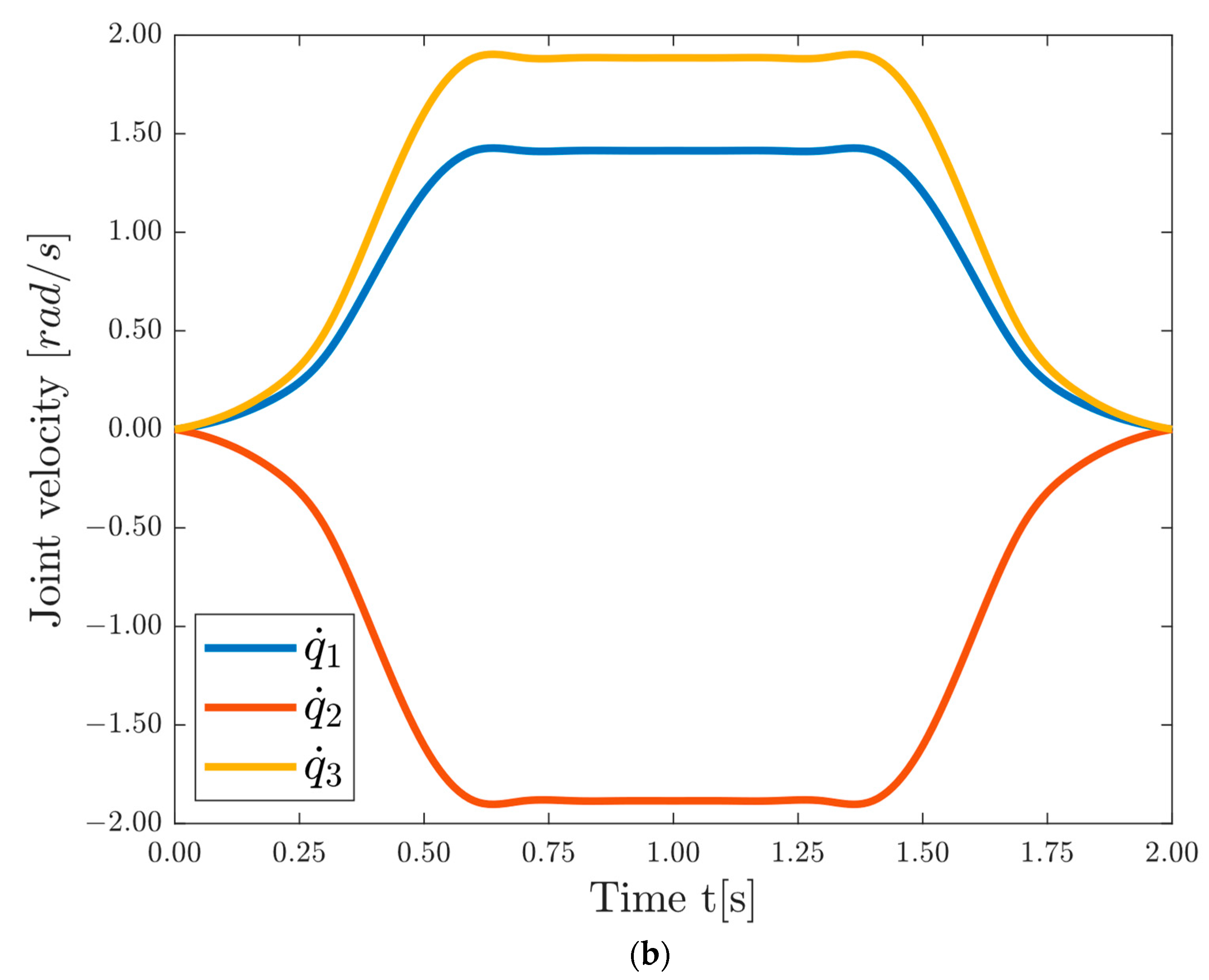
3.2.2. Computer Experiments

The computer experiments are conducted with MATLAB [30] and consider a scenario, where the gripper moves from point A (233, −172, 0) to point B (269, 155, 0) in the workspace. The equations of motion are used to compute the torques necessary to apply in the actuators in order to execute the work task. The desired movement from point A to point B is performed for 2 s by executing commands for applying the computed torques to the actuators in the joints. A trapezoidal motion profile for the variation of the velocities is employed to achieve smooth movement in the joints must smoothly increase. The desired maximal velocities and accelerations for the generalized coordinates $q_1, q_2 \mathrm{and} q_3$ are computed with respect to their physical hard constraints as follows: $1.4137 \left[\mathrm{rad}/\mathrm{s}\right], -0.0698 \left[\mathrm{rad}/\mathrm{s}\right],1.8850 \left[\mathrm{rad}/\mathrm{s}\right]$ and $4.1888 \left[\mathrm{rad}/{\mathrm{s}}^2 \right]$, $5.5851 \left[\mathrm{rad}/{\mathrm{s}}^2 \right]$ and $5.5851 \left[\mathrm{rad}/{\mathrm{s}}^2 \right]$. The displacement in the generalized coordinates, their velocities, accelerations and the torques required to perform the movement are visualized in Figure 9 and Figure 10. The torques ${\mathrm{T}}_1$, ${\mathrm{T}}_2$ and ${\mathrm{T}}_3$ reach their maximum values at time $t=0.4$ [s]. They are $0.4367 \left[\mathrm{Nm}\right]$, $0.0490 \left[\mathrm{Nm}\right]$ and $0.0846 \left[\mathrm{Nm}\right]$, respectively. When the torques are at the maximum, the accelerations in the first and the third joint also reach their maximum values.

4. Discussion

This paper presents a model of the dynamics of a robot arm with an open kinematic chain. The model makes use of the law of conservation of energy and the orthogonality principle to relate energy potential and energy flow characteristics attached to the edges of two non-intersecting graphs. These graphs have identical topological structures and serve to separate the representation of energy flow characteristics of displacement and rotation correspondingly. This approach allows to include in consideration all the external forces, torques and reactions applied to the links of a robot arm with arbitrary degrees of freedom. The graph notation employed to deal separately with displacement and rotation variables provides a uniform and intuitive approach to building the inherently complex model of dynamics. This paper proposes a procedure about how to apply this approach in the general case. Moreover, the implementation of the proposed procedure is demonstrated with a realistic case study. The case study considers a physical model of a robot arm constructed with a 3D printer in our laboratory. The objective of the case study has been to compute the drive torques for the execution of a required motion of the gripper given details of the geometrical and inertial characteristics of the robot arm. These equations of motion are obtained in closed form following the here proposed procedure. The results from computer experiments are provided and demonstrate that the robot arm gripper executes smoothly the required motion. Finally, it is worth mentioning that, unlike models of dynamics founded on the Lagrangian formulation, the proposed procedure allows to compute the reactions in the joints as well. Without loss of generality, in this case study, only rotational joints are taken into consideration. Dynamics in the case of the presence of translational joints can be modeled in a similar way. Finally, the scope of application of the here presented model can be further extended. It can be applied for the description of dynamics in other specific areas where the energy interaction occurs. For example, the elastic characteristics of the robot arm can be included in this model as well.

References

1. AlAttar, A.; Kormushev, P. Kinematic-Model-Free Orientation Control for Robot Manipulation Using Locally Weighted Dual Quaternions. Robotics 2020, 9, 76. [Google Scholar] [CrossRef]
2. Khalil, W. Dynamic Modeling of Robots using Recursive Newton-Euler Techniques. In Proceedings of the 7th International Conference on Informatics in Control, Automation and Robotics, Volume 1, Funchal, Madeira, Portugal, 15–18 June 2010; pp. 19–31. [Google Scholar]
3. Park, F.C.; Lynch, K.M. Modern Robotics. Mechanics, Planning and Control; Cambridge University Press: Cambridge, UK, 2017. [Google Scholar]
4. Xidias, E.K.; Aspragathos, N.A. Time sub-optimal path planning for hyper redundant manipulators amidst narrow passages in 3D workspaces. In Advances on Theory and Practice of Robots and Manipulators; Springer: Cham, Switzerland, 2014; pp. 445–452. [Google Scholar]
5. Valsamos, C.; Moulianitis, V.; Aspragathos, N. Kinematic Synthesis of Structures for Metamorphic Serial Manipulators. ASME J. Mechan. Robot. 2014, 6, 041005. [Google Scholar] [CrossRef]
6. Valsamos, C.; Wolniakowski, A.; Miatliuk, K.; Moulianitis, V.C. Minimization of Joint Velocities During the Execution of a Robotic Task by a 6 D.o.F. Articulated Manipulator. In Advances in Service and Industrial Robotics; Aspragathos, N.A., Koustoumpardis, P.N., Moulianitis, V.C., Eds.; Springer: Cham, Switzerland, 2019; Volume 67, pp. 368–375. [Google Scholar]
7. Bottin, M.; Rosati, G. Trajectory Optimization of a Redundant Serial Robot Using Cartesian via Points and Kinematic Decoupling. Robotics 2019, 8, 101. [Google Scholar] [CrossRef] [Green Version]
8. Jin, L.; Li, S.; La, H.; Luo, X. Manipulability optimization of redundant manipulators using dynamic neural networks. IEEE Trans. Indust. Electron. 2017, 64, 4710–4720. [Google Scholar] [CrossRef]
9. Dimeas, F. Singularity Avoidance in Human-Robot Collaboration with Performance Constraints. In Human-Friendly Robotics. Springer Proceedings in Advanced Robotics; Springer: Berlin/Heidelberg, Germany, 2020; Volume 18, pp. 89–100. [Google Scholar]
10. Rosati, G.; Boschetti, G.; Carbone, G. Advances in Mechanical Systems Dynamics. Robotics 2020, 9, 12. [Google Scholar] [CrossRef] [Green Version]
11. Carabin, G.; Wehrle, E.; Vidoni, R.A. Review on Energy-Saving Optimization Methods for Robotic and Automatic Systems. Robotics 2017, 6, 39. [Google Scholar] [CrossRef] [Green Version]
12. Kurdila, A.J.; Pinhas, B.-T. Dynamics and Control of Robotic Systems; John Wiley & Sons: Hoboken, NJ, USA, 2019. [Google Scholar]
13. Featherstone, R.; Orin, D. Robot Dynamics: Equations and Algorithms. In Proceedings of the IEEE International Conference Robotics & Automation, San Francisco, CA, USA, 24–28 April 2000; pp. 826–834. [Google Scholar]
14. Pryce, J.D.; Nedialkov, N. Another Multibody Dynamics in Natural Coordinates through Automatic Differentiation and High-Index DAE Solving. Acta Cybern. 2020, 24, 315–341. [Google Scholar] [CrossRef] [Green Version]
15. Neimark, J.I. Electromechanical analogies. Lagrange-Maxwell equations. In Mathematical Models in Natural Science and Engineering. Foundations of Engineering Mechanics; Springer: Berlin/Heidelberg, Germany, 2003. [Google Scholar] [CrossRef]
16. Kotev, V.; Boiadjiev, G.; Kawasaki, H.; Mouri, T.; Delchev, K.; Boiadjiev, T. Design of a hand-held robotized module for bone drilling and cutting in orthopedic surgery. In Proceedings of the 2012 IEEE/SICE International Symposium on System Integration (SII), Fukuoka, Japan, 16–18 December 2012; pp. 504–509. [Google Scholar] [CrossRef]
17. Guechi, E.-H.; Bouzoualegh, S.; Zennir, Y.; Blažič, S. MPC Control and LQ Optimal Control of A Two-Link Robot Arm: A Comparative Study. Machines 2018, 6, 37. [Google Scholar] [CrossRef] [Green Version]
18. Yovchev, K.; Delchev, K.; Krastev, E. State Space Constrained Iterative Learning Control for Robotic Manipulators. Asian J. Control 2018, 20, 1–6. [Google Scholar] [CrossRef]
19. Liang, B.; Li, T.; Chen, Z.; Wang, Y.; Liao, Y. Robot Arm Dynamics Control Based on Deep Learning and Physical Simulation. In Proceedings of the 37th Chinese Control Conference (CCC), Wuhan, China, 25–27 July 2018; pp. 2921–2925. [Google Scholar]
20. Franciosa, P.; Gerbino, S. A CAD-Based Methodology for Motion and Constraint Analysis According to Screw Theory. In Proceedings of the 2009 ASME International Mechanical Engineering Congress and Exposition. Volume 4: Design and Manufacturing, Lake Buena Vista, FL, USA, 13–19 November 2009; pp. 287–296. [Google Scholar] [CrossRef]
21. Damic, V.; Cohodar, M.; Kobilica, N. Development of Dynamic Model of Robot with Parallel Structure Based on 3D CAD Model. In Proceedings of the 30th DAAAM International Symposium, Vienna, Austria, 23–26 October 2019; pp. 155–160. [Google Scholar] [CrossRef]
22. Bejczy, A.K. Robot Arm Dynamics and Control; Technical memorandum 33-699, Jet Propulsion Laboratory; NASA: Washington, DC, USA, 1974.
23. Tellegen, B.D.H. A General Network Theorem, with Application. Philips Res. Rep. 1952, 7, 259–296. [Google Scholar]
24. Koenig, H.; Blackwell, W. Electromechanical System Theory; McGraw-Hill: New York, NY, USA, 1961. [Google Scholar]
25. Andrews, G. Dynamics Using Vector-Network Techniques; University of Waterloo, Department of Mechanical Engineering: Waterloo, ON, Canada, 1977. [Google Scholar]
26. Bojadjiev, G.; Lilov, L. Dynamics of Multicomponent Systems Based on the Orthogonality Principle. J. Theor. Appl. Mech. 1993, XXIV, 11–26. [Google Scholar]
27. Schmitke, C.; McPhee, J. Using linear graph theory and the principle of orthogonality to model multibody, multi-domain systems. Adv. Eng. Inform. 2008, 22, 147–160. [Google Scholar] [CrossRef]
28. Boiadjiev, G.; Kotev, V.; Delchev, K.; Boiadjiev, T. Modeling and Development of a Robotized Hand-Hold Bone Cutting Device OCRO. Int. J. Appl. Mech. Mater. 2013, 300–301, 479–483. [Google Scholar] [CrossRef]
29. Boiadjiev, G.; Chavdarov, I.; Miteva, L. Dynamics of a Planar Redundant Robot Based on Energy Conservation Law and Graph Theory. In Proceedings of the 2020 International Conference on Software, Telecommunications and Computer Networks (SoftCOM), Hvar, Croatia, 17–19 September 2020; pp. 1–6. [Google Scholar]
30. Corke, P. Robotics, Vision and Control. Fundamental Algorithms in MATLAB, 2nd ed.; Springer International Publishing: Berlin/Heidelberg, Germany, 2017. [Google Scholar]
Figure 1. Coordinate systems and vectors in two adjacent connected bodies.
Robotics 10 00128 g001
Figure 2. Graphs G p (left) and G r (right) of a free rigid body with mass center C .
Robotics 10 00128 g002
Figure 3. The topological structure of sub-graphs G p and G r of a robot arm with n DoF.
Robotics 10 00128 g003
Figure 4. Sequence of steps for deriving the differential equations of motion.
Robotics 10 00128 g004
Figure 5. Principal scheme of the robot arm.
Robotics 10 00128 g005
Figure 6. Simplified kinematic scheme of the robot arm.
Robotics 10 00128 g006
Figure 7. Topological structure of the 3 DoF robot arm.
Robotics 10 00128 g007
Figure 8. Incidence of edges and vertexes in graphs G p and G r .
Robotics 10 00128 g008
Figure 9. The calculated displacement(a) and the velocities of the generalized coordinates(b).
Robotics 10 00128 g009aRobotics 10 00128 g009b
Figure 10. The accelerations of the generalized coordinates(a) and the driving torques (b).
Robotics 10 00128 g010aRobotics 10 00128 g010b