Article

Reuleaux Triangle–Based Two Degrees of Freedom Bipedal Robot

Robotics and Mechatronics Laboratory, Department of Mechanical Engineering, Virginia Tech, Blacksburg, VA 24061, USA
*
Author to whom correspondence should be addressed.
Robotics 2021, 10(4), 114; https://doi.org/10.3390/robotics10040114
Submission received: 31 August 2021 / Revised: 8 October 2021 / Accepted: 12 October 2021 / Published: 16 October 2021
(This article belongs to the Special Issue Robotics: 10th Anniversary Feature Papers)

Abstract

:
This paper presents the design, modeling, analysis, and experimental results of a novel bipedal robotic system that utilizes two interconnected single degree-of-freedom (DOF) leg mechanisms to produce stable forward locomotion and steering. The single DOF leg is actuated via a Reuleaux triangle cam-follower mechanism to produce a constant body height foot trajectory. Kinematic analysis and dimension selection of the Reuleaux triangle mechanism is conducted first to generate the desired step height and step length. Leg sequencing is then designed to allow the robot to maintain a constant body height and forward walking velocity. Dynamic simulations and experiments are conducted to evaluate the walking and steering performance. The results show that the robot is able to control its body orientation, maintain a constant body height, and achieve quasi-static locomotion stability.

1. Introduction

To mimic the most commonly observed locomotion form in nature, legged robots have been a popular topic since the early days of robotic research. Leg designs with more active degrees of freedom (DOF) help to enhance the mobility and dexterity of legged robots [1], such as the ANYmal quadruped robot [2], the MIT Cheetah series quadruped robots [3,4], the Adaptive Suspension Vehicle [5], the ATRIAS robot [6], and the HyQ quadruped robot [7]. These robots utilize multiple DOFs per leg to position their (primarily) single-point-of-contact (SPOC) feet. The typical configuration of this type of legs uses three DOFs per leg [8,9], namely, one hip abduction/adduction DOF, one hip extension/flexion DOF, and one knee extension/flexion DOF (note that there are other types of leg configuration, such as those using parallel mechanisms [10].) Therefore, a multi-legged robot usually requires 6 n actuators, with n being the number of leg pairs. If non-SPOC feet are implemented, even more actuators are required to control the additional DOFs from the feet [11], which increases the robot complexity and the overall energy consumption [12].
To address the challenges of multiple DOFs leg mechanism, researchers have proposed the reduced-DOF leg designs which aim to utilize two or fewer active DOFs on each leg. This way, with fewer actuators, the overall weight and control complexity of the robotic system could be significantly reduced. For instance, Torige et al. [13] developed a centipede-like robot that consists of six segments. Each segment utilizes four motors to control two legs. Hoffman et al. [14] further promoted this concept by utilizing two passive revolute joints to couple the motion between two legs. This way, the two legs use only two linear actuators to extend the body, to lift the legs, and to drive the robot forward simultaneously. The RHex hexapod [15] robot is another typical reduced-DOF leg design which utilizes six continuously rotating C-shaped legs to drive the robot and uses a differential drive to achieve steering. Yoenda et al. [16] designed a quadruped robot with three active DOFs. This robot consists of a front and a rear section that can rotate about the orientation of the robot. The roll of each section, coupled with rotation of the U-shaped front and rear legs, allows the robot to move forward. Furthermore, single-DOF crank driven mechanisms [8,14,15,16,17,18,19,20,21], and two-DOF legs that generate an approximately straight-line support phase foot trajectories [22,23] have been proposed for the construction of legged robots for simplified control and design complexity. To build an easy-to-use and light legged platform for tail research purposes, the authors also proposed a reduced-DOF leg mechanism named Robotic Modular Leg (RML) [24,25], which has two DOFs per leg and can be implemented in a quadruped or biped robot in a modular manner. The “modular” in this context refers to the mechanical modules inside a robot, which is different from the more generalized “modular” concept that many independent modular robots constitute a larger robotic system. The RML leg mechanism applied decoupled actuation to simplify control and used a double parallelogram mechanism to keep the foot parallel to the robot chassis.
However, this design still requires two actuators, which is too heavy and too complicated (in terms of foot position planning) for the tail research [26]. Therefore, looking for a single DOF leg mechanism that is able to stably walk and steer becomes a practical requirement. However, by reviewing the literature, most existing single DOF leg mechanisms (such as the RHex robot [15] that was frequently used in robotic tail research [27]) are not able to maintain a constant body height, which induces instabilities during locomotion and thus is less attractive for our purpose.
Therefore, motivated by looking for a single DOF leg mechanism that can stably walk and steer, together with three additional requirements based on Kaneko [28], which are (1) to maintain quasi-static stability, (2) to maintain a constant robot body height, and (3) to maintain a constant body orientation, we propose a novel biped robot design, as shown in Figure 1. The new biped robot consists of two improved Robotic Modular Leg Mechanisms (the newer version in this paper is named RML-V2). The new idea relies on using the Reuleaux triangle cam-follower mechanism to couple the hip and knee motions of the old design. This way, the leg mechanism mobility is further simplified to one DOF, and the leg can generate a constant height trajectory due to the special Reuleaux triangle property. Although the cam-follower mechanism has been used in robot actuation [29], our application of the Reuleaux triangle cam-follower mechanism focuses on generating the foot trajectory with a straight-line support phase with minimum active DOFs. The angular orientation of the conjugate square is constrained via the two parallelogram mechanisms connected in series, which maintain the orientation without the use of an additional active DOF on the ankle. Thus, the leg mechanism can be used in conjunction with a flat foot support polygon to enable a quasi-static walking gait. It is worth noting that part of this work was previously published in [30]. The main contributions of this work are summarized as follows:
(1)
A novel single DOF leg mechanism that utilizes the Reuleaux triangle cam-follower mechanism to achieve constant body height during locomotion is proposed.
(2)
The mechanical design, kinematic analysis, dynamic modeling, prototyping, and experiments of a novel bipedal robot based on the novel leg mechanism are carried out, in order to verify the proposed leg mechanism.
The rest of this paper is organized as follows. Section 2 introduces the necessary knowledge of the Reuleaux triangle and presents the corresponding mechanical design of the RML-V2. Section 3 formulates the foot trajectory planning based on the synthesis of the Reuleaux triangle dimensions and its angular rotation. With the mechanical structure and the desired foot trajectory, dynamic analyses and corresponding simulations are presented in Section 4. Section 5 demonstrates a prototype of the proposed robot and presents the walking and steering experiments of the robot. Section 6 recaps the main novel points of the new leg design and concludes the paper.

2. Robotic Modular Leg—V2

This section reviews previous research on the design and implementation of the Reuleaux triangle (Section 2.1). The kinematic analysis of the Reuleaux triangle cam-follower mechanism is presented to formulate the analytical expressions of the foot trajectory, and the synthesis of the Reuleaux triangle dimensions which produce a desired step height and length (Section 2.2). Based on this kinematic knowledge, the main driving mechanism of the RML-V2 design is then presented in Section 2.3.

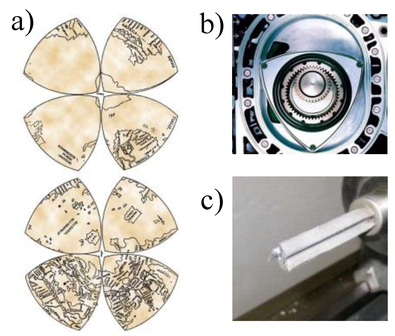
2.1. Reuleaux Triangle Background

The discovery and applications of the Reuleaux triangle trace back to the work of Leonardo da Vinci circa 1514 [31], when he made the Earth map consisting of eight triangular-shaped octants, as shown in Figure 2a. This octant shape was later defined by Franz Reuleaux in his book [32] in 1876 and then was used in Wankel internal combustion engine to produce suitable changing gas volumes in three chambers, as shown in Figure 2b. Harry J. Watts proposed to utilize the Reuleaux triangle property to cut square-shaped holes [33], as seen in Figure 2c, which was later studied by Figliolini et al. [34] and the analytical expressions describing the motion of particular points on the Reuleaux triangle during its rotation within a fixed conjugate square was formulated.

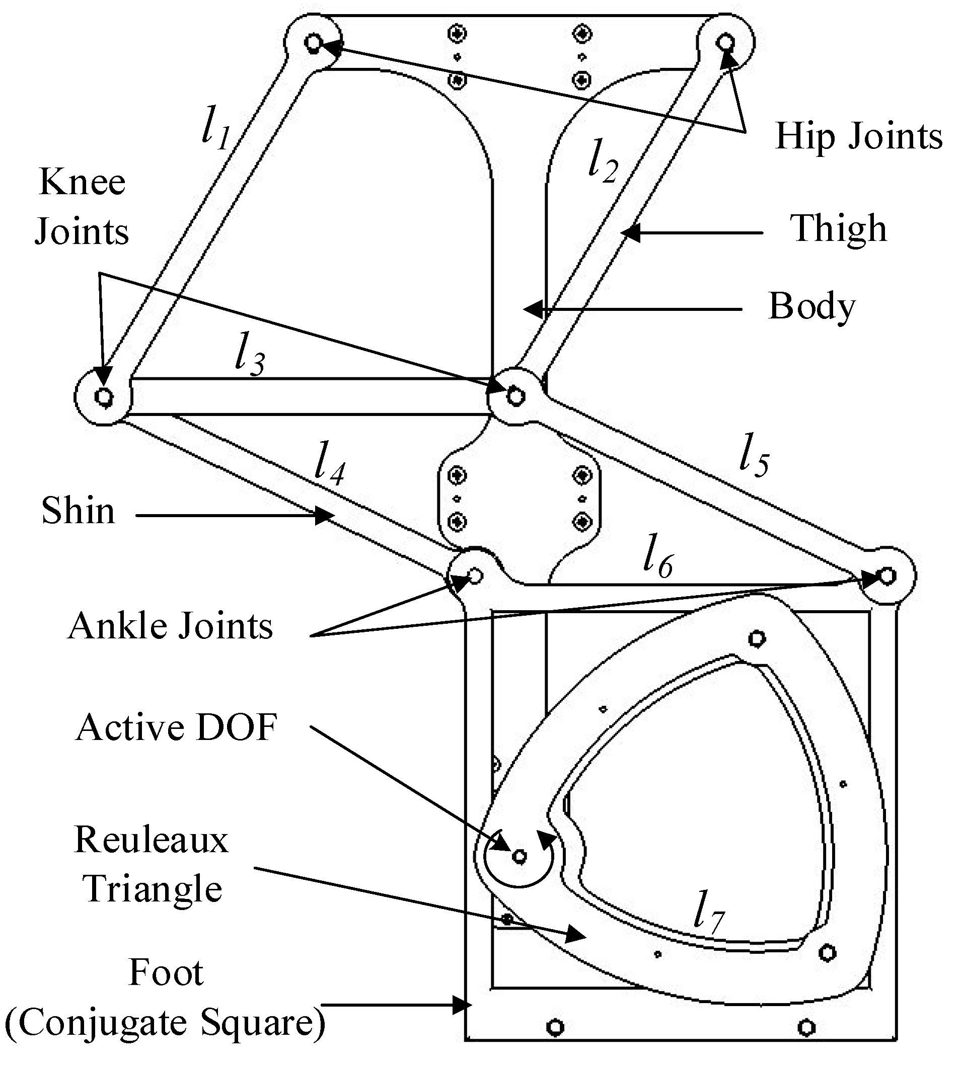
2.2. Kinematic Analysis

This section presents the kinematic analysis of the Reuleaux triangle (cam) and its foot follower (conjugate square). Prior applications [33] and analysis [34] mainly consider the motion of the Reuleaux triangle within a stationary conjugate square. However, in our usage of the Reuleaux triangle, the cam rotates about a point that is offset from its centroid to enable movement of the foot follower. Therefore, specific kinematic analysis is formulated first for this scenario. Based on the kinematic analysis, a desirable conjugate square centroid trajectory is produced such that it maintains a fixed orientation and a constant height. The leg mechanism dimensions are then synthesized to produce this desirable step length and height.
Figure 3 shows the schematic diagram of the Reuleaux triangle driving mechanism of the RML-V2, which is used to construct the biped robot. U , V , W are the three vertices of the Reuleaux triangle with each vertex coinciding its opposing arc center. The distance between any two vertices is l . The triangle rotates within a conjugate square with its four corners labelled as H , I , J , K and its centroid labelled as G . To ensure the conjugation between the Reuleaux triangle and its conjugate square, the length of the square sides should be also l [32]. This way, the Reuleaux triangle and its conjugate square form a two DOFs system such that the rotation of the triangle results in a planar displacement of the conjugate square in the inertial frame ( S ,   x ,   y ) . A body-attached frame of reference ( B ,   i 1 ,   i 2 ) is attached to the Reuleaux triangle at its centroid B , with i 1 pointing at U . The Reuleaux triangle rotates about a fixed-point O with an input angle α . Point O is offset from the centroid B by a distance ρ along i 1 .
The notation p j i represents the position of point j in frame i with i { B ,   S } . Furthermore, the scalar x - and y - components of an arbitrary vector z will be represented as z x and z y ( z = [ z x   z y ] T ) respectively. Note that in Figure 3, the Reuleaux triangle U V W is always in contact with the conjugate square. Therefore, the position vector of the conjugate square centroid G can be obtained from the position of the Reuleaux triangle vertices. The vertices contacting the conjugate square for α [ 0 ,   π / 2 ] are presented in Table 1.
We define the position vector p G S in the global reference frame based on the contact point of each vertex with the sides of the conjugate square. With reference to Table 1, Equation (1) is obtained to calculate the position vector p G S for α [ 0 ,   π / 2 ] . Note that due to the symmetric property of the Reuleaux triangle, the remaining phase ( α [ π / 2 ,   2 π ] ) of the trajectory profile can be generated by finding the corresponding contact points.
p G S = { ( p U S x l 2 ) x + ( p W S y + l 2 ) y ,                     α = [ 0 , π 6 )     ( p V S x + l 2 ) x + ( p W S y + l 2 ) y ,                     α = [ π 6 , π 3 ) ( p V S x + l 2 ) x + ( p U S y l 2 ) y ,                     α = [ π 3 , π 2 ]
The positions of U , V , W in Equation (1) can be obtained by mapping their positions from frame B to frame S using Equation (2).
p U S = R B S ( α ) ( ρ i 1 B + p U B ) + p O S p V S = R B S ( α ) ( ρ i 1 B + p V B ) + p O S p W S = R B S ( α ) ( ρ i 1 B + p W B ) + p O S
where R B S ( α ) is the rotation matrix from frame B to frame S with a given input angle α . The vertex positions in the body fixed frame B are defined in Equation (3).
p U B = l 3 i 1 B p V B = l 2 3 i 1 B + l 2 i 2 B p W B = l 2 3 i 1 B l 2 i 2 B
Substituting Equations (2) and (3) into Equation (1) yields the position of G with respect to the input angle α and offset ρ , as shown in Equation (4) where c α = cos α and s α = sin α .
p G S = { [ ( l 3 ρ ) c α l 2 ] x + [ l 6 ( 3 l + 6 ρ ) S α + l 2 ( 1 C α ) ] y ,                     α = [ 0 , π 6 )     [ ( l 2 ( 1 S α ) l 6 ( l 3 + 6 ρ ) C α ] x + [ l 6 ( 3 l + 6 ρ ) S α + l 2 ( 1 C α ) ] y ,                     α = [ π 6 , π 3 ) [ ( l 2 ( 1 S α ) l 6 ( l 3 + 6 ρ ) C α ] x + [ ( l 3 ρ ) S α l 2 ] y ,                     α = [ π 3 , π 2 ]
Based on Equation (4), the point G trajectories π i are illustrated in Figure 4 for various offset values of ρ . The profiles are normalized with respect to the triangle length l . Note that the trajectory profile varies with respect to different offsets, ρ . The trajectories π 1 , π 2 , π 3 , π 4 , and π 8 are shown in Figure 4a and the trajectories π 5 , π 6 , and π 7 are shown in Figure 4b. The characteristics of these profiles were investigated and presented in Reuleaux’s original book [32] that the ρ = | B U | yields π 1 , a straight-sided quadrilateral profile with corners that are elliptically rounded, as shown in Figure 4a. For values of ρ satisfying the inequality 0.5 ( l | B U | ) < ρ < | B U | , the trajectories π 2 and π 3 are obtained and represent a concaved sided quadrilateral with round corners. For ρ = 0.5 ( l | B U | ) , the trajectory denoted as π 4 represents a super ellipse or Lamé curve.
Similarly, for the profiles in Figure 4b, when ρ value satisfies the inequality ( | B U | l / 2 ) < ρ < 0.5 ( l | B U | ), the trajectory π 5 consists of four intersecting concave elliptical curves which form four loops. When ρ value approaches ( | B U | l / 2 ), the loops expand and eventually are tangent to each other at ρ = ( | B U | l / 2 ) . This home central form of π 5 is π 6 trajectory. For 0 < ρ < ( | B U | l / 2 ) , the four elliptical curves intersect with each other and form the π 7 trajectory. For ρ = 0 , the π 8 trajectory consists of four convex elliptical curves which are tangent to its neighboring curves [32].

2.3. Mechanical Design

Figure 5 shows a side view schematic diagram of the RML-V2. The leg consists of two serially connected parallelogram mechanisms with one being the thigh and the other being the shin. The thigh parallelogram rotates about the hip joint and the shin parallelogram rotates about the knee joint. Due to the parallelogram mechanism, the foot maintains a constant orientation with respect to the body without requiring an additional DOF at the ankle. The size of the foot is chosen to be large enough so that the leg could be statically stable during the support phase. The above presented Reuleaux triangle cam-follower mechanism is placed inside the foot to actuate the RML-V2. The Reuleaux triangle rotates about an axis on the body (the active DOF shown in Figure 5) and thus drives the conjugate square foot to form a quasi-square trajectory, which will be discussed in Section 3. These design features improve the first generation of the RML [24,25] by reducing the two active DOFs to one and generating a foot trajectory with a constant body height. The single DOF actuation facilitates the control system development, and the constant body height foot trajectory makes the locomotion more stable. However, these improvements are mainly based on the flat surface and the quasi-static condition. That is, the robot moves slowly enough so that its dynamic effect is minimized, and the large foot design guarantees that the system center of mass is always inside the supporting polygon.

3. Foot Trajectory Planning

To maintain constant body height and walking speed during locomotion, the foot trajectory planning is discussed in this section. Both the swing phase and the support phase foot trajectories are generated in space relative to the legged robot body. The support phase is defined as the foot trajectory portion that is in contact with the ground, while the swing phase is the portion when the foot is in the air. Since the RML-V2 is a single DOF mechanism with a fixed foot (conjugate square) trajectory, based on the kinematics in Section 2.2, the planning process involves: (1) selecting the optimal α ( t ) for the foot with various values of ρ , (2) synthesizing mechanism design parameters to obtain a desirable step length and step height, and (3) designing the gait sequence for bipedal locomotion.

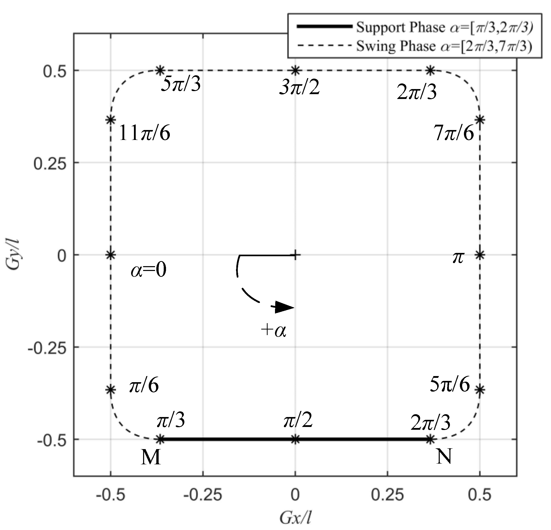
3.1. Single Leg Foot Trajectory Planning

As discussed in Section 2, it is desirable to let the robot maintain a constant body height and orientation such that the energy consumption for a forward walking gait could be minimized. This requires a straight-line support phase for the foot trajectory [28]. Referring to Figure 4a, trajectory profile π 1 illustrates a straight-sided quadrilateral such that one of the straight sides can be used as the straight-line support phase foot trajectory. Therefore, the offset distance from the Reuleaux triangle centroid B to the rotational center O should be set to ρ = | B U | = l / 3 .
For clarity, the stroke length and the stroke height are defined as the maximum range of horizontal and vertical distances shown on the trajectory profile, while the step length and the step height are defined as the horizontal and vertical distances corresponding to the support phase and the swing phase. For instance, in Figure 4a, the distance between point M and point N on the π 1 trajectory defines the step length, while the distance between the two vertical sides defines the stroke length.
Based on Equation (4) and Figure 6, for α [ 0 ,   π / 6 ) , the trajectory profile is represented as a vertical straight line with x -component equivalent to l / 2 , for α [ π / 6 ,   π / 3 ) , the profile is an elliptical curve, and for α [ π / 3 ,   π / 2 ] , the profile is a horizontal straight line with the y -component equivalent to l / 2 . Due to the symmetric property of the Reuleaux triangle cam-follower mechanism presented in Section 2, the other three quadrants of the foot trajectory can be generated by mirroring the α [ 0 ,   π / 2 ] portion with respect to the x -axis first and then with respect to the y -axis. Both the stroke height and the stroke length are l .
As shown in Figure 6, the support phase (highlighted by thick solid line) of the foot trajectory initiates at α = π / 3 and terminates at α = 2 π / 3 . Substituting these values into Equation (4) yields the coordinates of points M and N . Therefore, the step length is calculated as l ( 3 1 ) . These relations could be used to synthesize the dimensions of the Reuleaux triangle mechanism such that a desirable step length and height is achieved.

3.2. Gait Sequencing for Bipedal Locomotion

This section analyzes the additional requirements of the input angle α trajectory such that the RML-V2 achieves a constant body height as well as a constant walking velocity during the support phase. As stated in Section 3.1, the foot trajectory π 1 is selected to ensure a constant body height for the support phase. Since each leg has only one DOF, to avoid motion conflict during forward motion, the two feet should not have different speeds when the feet are both on the ground. Otherwise, the robot body may fluctuate vertically and cause instances of instability. Moreover, to minimize variations in acceleration, it is desirable to have a constant forward velocity for walking gaits. Therefore, this section provides the design of the gait sequencing of the two legs such that the biped achieves stable forward walking with a constant speed v .
Referring to Figure 6, the gait cycle period is the sum of the times for the support and swing phases. In this work, we set the support phase time to be equal to the swing phase time. Therefore, the gait cycle period, for a combined single swing and single support phase, can be obtained from Equation (5).
T = 2 | M N | v = l v ( 2 3 2 )
With the assumption of no slipping condition, the walking velocity v of the robot equals to the velocity of the conjugate square, which could be obtained from taking the time derivative of p G S . Therefore, based on Equation (4), differentiating p G S during the support phase ( π / 3 α π / 2 ) yields the horizontal velocity of the conjugate square for half of the support phase, as shown in Equation (6).
d α d t l 2 cos ( α ) + d α d t 3 2 l sin ( α ) = v
Substitute Equation (5) into Equation (6) and define τ = t / T to be the completed percentage of a gait cycle. Define τ s p p o r t as the duty cycle and τ s w i n g = 1 τ s p p o r t . Since τ s p p o r t is set to be equal to τ s w i n g , τ s p p o r t = 0.5 . Using these relations, solving α from Equation (6) yields Equation (7) for π / 3 α < π / 2 , and Equation (8) for π / 2 α 2 π / 3 , respectively.
α = arcsin ( ( 2 3 2 ) τ C 1 ) + 2 π 3 ,           α [ π 3 , π 2 )
α = arcsin ( ( 2 3 2 ) τ C 2 ) + π 3 ,               α [ π 2 , 2 π 3 ]
Here, C 1 and C 2 are the constants of integration that can be obtained from initial conditions where the transition from the support phase to the swing phase occurs, and vice versa. To achieve smooth transitions from the support phase to the swing phase, cubic splines are interpolated to generate the rotation angle trajectory α ( t ) of the Reuleaux triangle in the time domain for a swing phase that satisfies τ s w i n g = 0.5 .

4. Dynamic Analysis of the Robotic System

This section presents the dynamic analysis of the biped robot. The dynamic model of the robot is obtained using Kane’s method [35]. Since the robot consists of planar mechanisms, for each of the bodies shown in Figure 5, four parameters are defined—three Cartesian coordinates and one rotation angle. Hence, the linear velocity and angular velocity can be calculated as
v k = J v k q ˙ ω k = J ω k q ˙
where q = [ q 1 , q 2 ] T = [ α 1 , α 2 ] T are the generalized coordinates. J v k and J ω k are the Jacobians of the k -th link (labelled as l k in Figure 5) corresponding to v k and ω k respectively. The inertia force of the k -th link is F k * = m a k , and the inertia torque is T k * = ( I k α k + ω k × I k ω k ) where a k , α k , and Ik are the linear acceleration, angular acceleration, and the inertia matrix of the k -th link, respectively. Therefore, the generalized inertia force of the k -th link is obtained as K k * = J v k T F k * + J ω k T T k * , which is further expanded as
K k * = M k q ¨ ( J v k T m i J ˙ v k + J ω k T m k J ˙ ω k ) q ˙ J ω k T ω ˜ k I k ω k
where Mk is the inertia matrix calculated as M k = J v k T m k J v k + J ω k T I k J ω k and ω ˜ k is the skew-symmetric matrix of ω k . The external forces applied to the body are the gravity and the input torques τ l , τ r , which drive the Reuleaux triangle cam on the left leg and the right leg, respectively. The generalized external force is calculated as:
K k = J v k T m k g + J ω k T τ l + J ω k T τ r
The equation of motion of the robot is then derived with J C T as the transpose of the constraint Jacobian and λ as the Lagrange multiplier, as shown in Equation (12). Here, the Lagrange multiplier presents the constraint force caused by the friction and support of the ground during walking. The Lagrange multiplier is a function of q that eliminates the switch between two conditions where the left foot or the right foot is in contact with the ground.
K k + K k * + J C T λ = 0
A Proportional-Integral (PI) compensator is utilized to generate an input torque such that the Reuleaux triangle cams can track the desired foot trajectory described in Section 3. Simulation of the robot walking is performed using MATLAB. The cam mass is set to 0.209 kg, the foot mass to 0.427 kg and the body mass to 1.319 kg. The mass of the remaining robot components is assumed to be negligible. The walking gait cycle was set to 4 s. Initial conditions are q = [ π / 6 , π / 3 ] T and q ˙ = [ 0 ,   0 ] T when one foot initiates the support phase, and the other foot initiates the swing phase. The tracking results of the Reuleaux triangle cam for two gait cycles are presented in Figure 7.
In Figure 7, the blue dash line represents the simulated rotation angle of the Reuleaux triangle cams, and the black solid line is the desired angle trajectory described in Section 3. The average tracking error of the controller for the left foot is 0.0079 radians with a standard deviation of 0.0085 radians, and the average tracking error of the right foot is 0.0078 radians with a standard deviation of 0.0085 radians.
Figure 8 shows the corresponding control efforts on the motor to track the trajectory in Figure 7. The motor torque reaches a maximum during the swing phase of a gait cycle to overcome the gravitational and frictional loading on the foot. During the support phase, the motor torque is mainly used to overcome the friction between the Reuleaux triangle and its conjugate square foot.

5. Experimental Results

This section presents the integration of the RML-V2 prototype (Section 5.1) and the walking experiments of the prototype (Section 5.2).

5.1. Robot Prototype
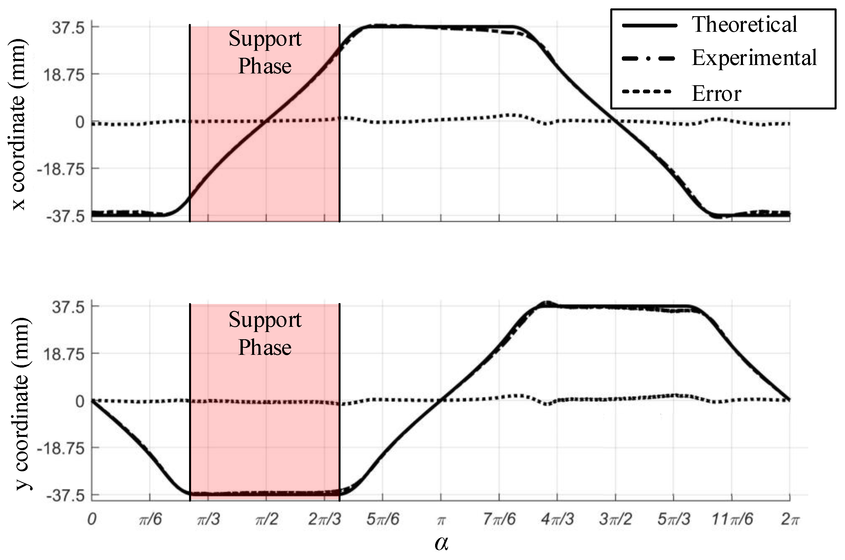
A prototype of the RML-V2 was built to verify the mechanism design and to evaluate the performance of the robot. Acrylonitrile Butadiene Styrene (ABS) based 3D printing was used to manufacture the prototype parts. Two Dynamixel MX-106 smart actuators were used to drive the Reuleaux triangle cams. The prototype measures 230 × 200 × 320 mm and weighs 2.5 kg in total. The Reuleaux triangle dimensions are selected to produce a gait cycle with a step height of 75 mm, and a step length of 54.9 mm.
The prototype was first fixed to a stable surface to measure its actual foot trajectory. The measurement was achieved by tracking a blue marker attached on the foot via computer vision method. The Reuleaux triangle cam was set to rotate at a constant velocity. Tracking results versus theoretical results are presented in Figure 9 where the actual foot trajectory is presented as dashed lines, and the theoretical trajectory π 1 is presented as solid lines. Furthermore, Figure 10 presents the tracking error in the x - and y -coordinates with respect to the rotation angle α , along with the theoretical trajectories for the foot rotation cycle.
In Figure 10, the error shows a relatively straight line around zero. During the swing phase, the average error of the x -coordinate is 0 mm with a standard deviation of 0.86 mm and the average error of the y -coordinate is 0.03 mm with a standard deviation of 0.82 mm. During the support phase, the average y -coordinate error is −0.61 mm with a standard deviation of 0.11 mm. Therefore, it can be concluded that the actual support phase foot trajectory of the prototype is a straight line.

5.2. Indoor Walking

As discussed in Section 3, the input angle trajectories and the gait sequences are designed to produce a constant forward velocity and to satisfy actuation capabilities. The prototype was placed on an indoor floor and a 5 s gait cycle was selected for the testing. According to Equation (5), the robot walking speed is determined to be 21.9 mm/s. Using the same computer vision method in the previous subsection, the robot body horizontal ( x ) and vertical ( y ) displacements with respect to time was obtained and presented in Figure 11. The walking snapshots are presented in Figure 12A–F, and a corresponding video could be found in the Supplementary Materials. In Figure 11, the x and y displacements of the robot body during walking show a linear pattern with respect to time. Regression technique reveals that the correlation coefficient is 0.99 for both x and y displacements, which means that the robot walks at a constant velocity and with a constant body height. Therefore, the prototype is concluded to meet the criteria of having a constant velocity. Further analysis of the dataset shows that the speed of the robot is 21 mm/s, which is very close to the desired walking speed of 21.9 mm. The steering (differential turning) was conducted by locking one foot of the robot in the support phase while the other foot is engaged in a full gait cycle. This generated an 18 degrees reorientation of the robot, which is shown in Figure 12G–L.
As demonstrated in these experiments, the biped robot, which is composed of two single-DOF RML-V2 mechanisms, meets all the design requirements discussed in Section 1. That is, the robot achieves a quasi-static stability on a flat surface while maintaining a constant robot body height and a constant body orientation. The tested results also validated the kinematic analysis (through experimental results in Figure 9 and Figure 10) in Section 2 and the leg motion planning (through experimental results in Figure 12) in Section 3. One observed deficiency is, however, that the biped also requires smooth surface during steering. This is mainly due to the fact that the single DOF leg relies on motion confliction (through ground friction) to change direction. However, this is an inevitable disadvantage as the tradeoff of the reduced mobility.

6. Conclusions

This paper presented the design and implementation of a novel biped robot based on a new single DOF robotic leg mechanism named RML-V2. The RML-V2 utilizes the classic Reuleaux triangle cam-follower mechanism and a double parallelogram mechanism, which is used to restrict the rotation motion of the conjugate square of the Reuleaux triangle mechanism so that the foot is always in parallel with the ground during a gait cycle. Corresponding kinematics of the leg mechanism was derived based on the Reuleaux triangle geometry and a foot trajectory that can guarantee a constant body height and a steady forward velocity was selected. Dynamics model of the bipedal robot was derived, and corresponding walking simulation was performed to verify the design. To practically validate the proposed mechanism and evaluate the theoretical analysis, a prototype was built and various experiments were carried out. The results showed that the robot meets all the design requirements and is able to produce a stable quasi-static forward walking gait as well as an effective differential turning motion.

Supplementary Materials

A supplementary video showing the working prototype is available online at https://www.youtube.com/watch?v=Yny7gS1V9Fg.

Author Contributions

Conceptualization, W.S. and P.B.-T.; methodology, J.Y. and W.S.; validation, J.Y.; data curation, J.Y.; writing—original draft preparation, J.Y.; writing—review and editing, Y.L.; supervision, P.B.-T.; project administration, P.B.-T.; funding acquisition, P.B.-T. All authors have read and agreed to the published version of the manuscript.

Funding

This research was funded by National Science Foundation, grant number 1557312 and 1906727.

Institutional Review Board Statement

Not applicable.

Informed Consent Statement

Not applicable.

Data Availability Statement

The data presented in this study are available upon reasonable request from the corresponding author.

Acknowledgments

The authors also would like to thank Jiamin Wang for the assistance in dynamic analysis, Zhoubao Pang, and Hongxu Guo for their assistance in making the prototype and Shubhdildeep Sohal for his assistance in the experimental set up and data collection.

Conflicts of Interest

The authors declare no conflict of interest.

References

  1. Silva, M.F.; MacHado, J.A.T. A historical perspective of legged robots. J. Vib. Control 2007, 13, 1447–1486. [Google Scholar] [CrossRef] [Green Version]
  2. Hutter, M.; Gehring, C.; Jud, D.; Lauber, A.; Bellicoso, C.D.; Tsounis, V.; Hwangbo, J.; Bodie, K.; Fankhauser, P.; Bloesch, M.; et al. ANYmal—A highly mobile and dynamic quadrupedal robot. In Proceedings of the IEEE International Conference on Intelligent Robots and Systems, Daejeon, Korea, 9–14 October 2016. [Google Scholar]
  3. Seok, S.; Wang, A.; Chuah, M.Y.; Hyun, D.J.; Lee, J.; Otten, D.M.; Lang, J.H.; Kim, S. Design principles for energy-efficient legged locomotion and implementation on the MIT cheetah robot. IEEE/ASME Trans. Mechatron. 2014, 20, 1117–1129. [Google Scholar] [CrossRef] [Green Version]
  4. Katz, B.; Di Carlo, J.; Kim, S. Mini cheetah: A platform for pushing the limits of dynamic quadruped control. In Proceedings of the International Conference on Robotics and Automation, Montreal, QC, Canada, 20–24 May 2019. [Google Scholar]
  5. Waldron, K.J.; McGhee, R.B. The adaptive suspension vehicle. IEEE Control Syst. Mag. 1986, 6, 7–12. [Google Scholar] [CrossRef]
  6. Hubicki, C.; Grimes, J.; Jones, M.; Renjewski, D.; Spröwitz, A.; Abate, A.; Hurst, J. ATRIAS: Design and validation of a tether-free 3D-capable spring-mass bipedal robot. Int. J. Robot. Res. 2016, 35, 1497–1521. [Google Scholar] [CrossRef]
  7. Semini, C.; Tsagarakis, N.G.; Vanderborght, B.; Yang, Y.; Caldwell, D.G. HyQ-hydraulically actuated quadruped robot: Hopping leg prototype. In Proceedings of the 2nd Biennial IEEE/RAS-EMBS International Conference on Biomedical Robotics and Biomechatronics, Scottsdale, AZ, USA, 19–22 October 2008. [Google Scholar]
  8. Kaneko, M.; Abe, M.; Tanie, K.; Tachi, S.; Nishizawa, S. Basic experiments on a hexapod walking machine (MELWALK-III) with an approximate straight-line link mechanism. In Proceedings of the International Conference on Advanced Robotics, St. Louis, MO, USA, 9–10 September 1985. [Google Scholar]
  9. Nelson, G.M.; Quinn, R.D. Posture control of a cockroach-like robot. IEEE Control Syst. Mag. 1999, 19, 9–14. [Google Scholar]
  10. Wang, S.; Chen, Z.; Li, J.; Wang, J.; Li, J.; Zhao, J. Flexible motion framework of the six wheel-legged robot: Experimental results. IEEE/ASME Trans. Mechatron. 2021, in press. [Google Scholar] [CrossRef]
  11. Schwab, A.L.; Wisse, M. Basin of attraction of the simplest walking model. In Proceedings of the International Design Engineering Technical Conferences and Computers and Information in Engineering Conference, Pittsburgh, PA, USA, 9–12 September 2001. [Google Scholar]
  12. Galvez, J.A.; Estremera, J.; De Santos, P.G. A new legged-robot configuration for research in force distribution. Mechatronics 2003, 13, 907–932. [Google Scholar] [CrossRef]
  13. Torige, A.; Noguchi, M.; Ishizawa, N. Centipede type multi-legged walking robot. In Proceedings of the IEEE/RSJ International Conference on Intelligent Robots and Systems, Yokohama, Japan, 26–30 July 1993. [Google Scholar]
  14. Hoffman, K.L.; Wood, R.J. Passive undulatory gaits enhance walking in a myriapod millirobot. In Proceedings of the IEEE International Conference on Intelligent Robots and Systems, San Francisco, CA, USA, 25–30 September 2011. [Google Scholar]
  15. Saranli, U.; Buehler, M.; Koditschek, D.E. RHex: A simple and highly mobile hexapod robot. Int. J. Robot. Res. 2001, 20, 616–631. [Google Scholar] [CrossRef] [Green Version]
  16. Yoneda, K.; Ota, Y.; Ito, F.; Hirose, S. Construction of a quadruped with reduced degrees of freedom. In Proceedings of the Industrial Electronics Conference, Nagoya, Japan, 22–28 October 2000. [Google Scholar]
  17. Funabshi, H.; Ogawa, K.; Gotoh, Y.; Kojima, F. Synthesis of leg-mechanisms of biped walking machines: Part i, synthesis of ankle-path-generator. Bull. JSME 2011, 28, 537–543. [Google Scholar] [CrossRef]
  18. Liang, C.; Ceccarelli, M.; Takeda, Y. Operation analysis of a one-dof pantograph leg mechanisms. In Proceedings of the 17th International Workshop on Robotics in Alpe-Adria-Danube Region, Ancona, Italy, 15–17 September 2008. [Google Scholar]
  19. Tavolieri, C.; Ottaviano, E.; Ceccarelli, M.; Di Rienzo, A. Analysis and design of a 1-dof leg for walking machines. Proc. RAAD 2006, 6, 63–71. [Google Scholar]
  20. Liu, Y.; Ben-Tzvi, P. An articulated closed kinematic chain planar robotic leg for high-speed locomotion. J. Mech. Robot. 2020, 12, 041003–041018. [Google Scholar] [CrossRef]
  21. Park, J.; Kim, K.S.; Kim, S. Design of a cat-inspired robotic leg for fast running. Adv. Robot. 2014, 28, 1587–1598. [Google Scholar] [CrossRef]
  22. Adachi, H.; Koyachi, N.; Nakano, E. Mechanism and control of a quadruped walking robot. IEEE Control Syst. Mag. 1988, 8, 14–19. [Google Scholar] [CrossRef]
  23. Ch, L.E.; Pop, C.; Pop, F.; Dolga, V. Novel solution for leg motion with 5-link belt mechanism. Int. J. Appl. Mech. Eng. 2014, 19, 699–708. [Google Scholar] [CrossRef] [Green Version]
  24. Saab, W.; Ben-Tzvi, P. Design and analysis of a robotic modular leg mechanism. In Proceedings of the International Design Engineering Technical Conferences and Computers and Information in Engineering Conference, Charlotte, NC, USA, 21–24 August 2016. [Google Scholar]
  25. Saab, W.; Rone, W.; Ben-Tzvi, P. Robotic modular leg: Design, analysis, and experimentation. J. Mech. Robot. 2017, 9, 024501–024506. [Google Scholar] [CrossRef]
  26. Rone, W.S.; Saab, W.; Kumar, A.; Ben-Tzvi, P. Controller Design, Analysis, and Experimental Validation of a Robotic Serpentine Tail to Maneuver and Stabilize a Quadrupedal Robot. J. Dyn. Syst. Meas. Control 2019, 141, 081002. [Google Scholar] [CrossRef] [Green Version]
  27. Libby, T.; Johnson, A.M.; Chang-Siu, E.; Full, R.J.; Koditschek, D.E. Comparative design, scaling, and control of appendages for inertial reorientation. IEEE Trans. Robot. 2016, 32, 1380–1398. [Google Scholar] [CrossRef]
  28. Kaneko, M.; Abe, M.; Tachi, S.; Nishizawa, S.; Tanie, K.; Komoriya, K. Legged locomotion machine based on the consideration of degrees of freedom. Theory Pract. Robot. Manip. 2012, 403–410. [Google Scholar] [CrossRef]
  29. Sun, Q.; Wang, C.; Zhao, D.; Zhang, C. Cam drive step mechanism of a quadruped robot. J. Robot. 2014, 2014, 851680. [Google Scholar] [CrossRef] [Green Version]
  30. Yang, J.; Saab, W.; Ben-Tzvi, P. A two-dof bipedal robot utilizing the reuleaux triangle drive mechanism. In Proceedings of the IEEE/RSJ International Conference on Intelligent Robots and Systems, Macau, China, 3–8 November 2019. [Google Scholar]
  31. Bower, D.I. The unusual projection for one of john dee’s maps of 1580. Cartogr. J. 2012, 49, 55–61. [Google Scholar] [CrossRef]
  32. Reuleaux, F. Kinematics of Machinery: Outlines of a Theory of Machines; Dover Publications Inc.: New York, NY, USA, 1963. [Google Scholar]
  33. Watts, H.J. Drill or Boring Member. U.S. Patent 1,241,176, 25 September 1917. [Google Scholar]
  34. Figliolini, G.; Rea, P.; Grande, S. Higher-pair reuleaux-triangle in square and its derived mechanisms. In Proceedings of the International Design Engineering Technical Conferences and Computers and Information in Engineering Conference, Chicago, IL, USA, 12–15 August 2012. [Google Scholar]
  35. Featherstone, R. Rigid Body Dynamics Algorithms; Springer: Berlin, Germany, 2014. [Google Scholar]
Figure 1. The design concept of the biped robot constructed with two RML-V2 mechanisms.
Robotics 10 00114 g001
Figure 2. Applications of Reuleaux triangle: (a) Earth map made by da Vinci, (b) Wankel internal combustion engine, and (c) Square hole cutting tool.
Robotics 10 00114 g002
Figure 3. Schematic diagram of the Reuleaux triangle and its conjugate square.
Robotics 10 00114 g003
Figure 4. Trajectory profiles of point G normalized with respect to l for various offset values ρ : (a) five profiles without self-intersection, and (b) three profiles with self-intersection. The stars (M and N) in the figure indicate the endpoints of the support phase trajectory.
Robotics 10 00114 g004
Figure 5. Side view schematic diagram of the RML-V2.
Robotics 10 00114 g005
Figure 6. Foot trajectory profile with input angle α where the stars represent the points on the trajectory that correspond to the evenly distributed α value of π / 6 .
Robotics 10 00114 g006
Figure 7. Simulated PI compensator tracking results.
Robotics 10 00114 g007
Figure 8. Calculated torque on both motors.
Robotics 10 00114 g008
Figure 9. Experimental and calculated foot trajectory where the cross in the center indicates the symmetric center of the trajectory, which is also the rotation center of the Reuleaux triangle cam.
Robotics 10 00114 g009
Figure 10. x - and y -coordinate errors of experimental results versus theoretical results.
Robotics 10 00114 g010
Figure 11. Straight walking prototype body x and y displacement.
Robotics 10 00114 g011
Figure 12. Biped robot demonstrating forward locomotion (AF), and differential turning (GL).
Robotics 10 00114 g012
Table 1. Conjugate square side that Reuleaux triangle vertices land on for α [ 0 ,   π / 2 ] .
Rotation Angle α U V W
α [ 0 ,   π / 6 ] I J Inside the square K J
α [ π / 6 ,   π / 3 ] Inside the square H K K J
α [ π / 3 ,   π / 2 ] H I H K Inside the square
Publisher’s Note: MDPI stays neutral with regard to jurisdictional claims in published maps and institutional affiliations.

