1. Introduction
Detailed knowledge of robot dynamic parameters can be beneficial for several applications. However, in contrast with the kinematic ones, these values are usually not fully provided by the manufacturer. As an example, Universal Robots, one of the main brands in collaborative robotics, details only the expected values of the mass and the position of the center of mass of each joint/link of its manipulators [
1], for a total of 24 (4 × 6) parameters. On the other hand, the remaining 54 (9 × 6), which include links and motors inertia and Coulomb and viscous friction, remain unknown, thus preventing the definition of accurate dynamic models. According to [
2,
3], this is of primary importance for control algorithms currently adopted for industrial manipulators which often rely on control strategies far more complex than simple Proportional-Integral-Differential (PID) ones [
4]. On the other hand, a different approach could be derived from [
5], where deterministic artificial intelligence has been effectively used to learn the dynamic properties of an unmanned underwater vehicle for autonomous trajectory generation and control.
Moreover, an imprecise estimate of the torques required to execute the desired trajectory could negatively influence the effectiveness of algorithms used to provide performance indexes to evaluate the energy consumption of a manipulator [
6], or to define optimal trajectories to minimize the power required by the robot without compromising its productivity [
7,
8]. Since these methods use the Lagrange formulation [
9], more accurate knowledge of the dynamic parameters of the robot arm could lead to a better estimate of the joints torques.
High-Fidelity (HF) mathematical models could be also used for diagnostics and prognostics purposes. To do so, most of the algorithms currently employed rely on data-driven methods, which need to be trained on large data sets representative of the statistical distribution of the system behavior in both nominal and off-nominal conditions [
10]. However, since the Mean Time Between Failures (MTBF) of a robot is in the order of tens of thousands of hours [
11], there is a general lack of data associated with operation under degraded health conditions. To overcome this limitation, and quickly generate extensive data sets through which design and evaluate dedicated prognostic routines, simulated faults and failures can be inserted in the HF model of the manipulator. The effectiveness of this approach in industrial robots applications is discussed in [
12], where prognostics routines have been applied to predict fault and failures in a roller hemming head mounted on a 5 DOF manipulator. Given these premises, reliable results can be obtained through the exact definition of both the kinematic and dynamic parameters of the robot arm, as well as through the modeling of its components.
Diagnostics and prognostics algorithms are crucial not only to minimize downtimes and economical losses in production or assembly lines, but also to guarantee the safety of the operator who is sharing his workspace with the robot. Despite the old idea of industrial automation where robots are surrounded by fences and cages to which access is usually restricted, in tasks involving Human–Robot Collaboration (HRC), the worker and the machine operate in close proximity as in the case of hand-over applications analyzed in detail in [
13]. According to the norms in force, such cooperation is feasible only if the operator’s safety is always guaranteed. A possible solution consists of preventing an impact between the operator and the robot arm by implementing collision avoidance algorithms [
14,
15]. An example of a practical implementation of this approach has been proposed by [
16], where a human–robot assembly task is disclosed. However, especially in the case of continuous cooperation of the worker and the robot, advanced algorithms for human–robot workspace sharing cannot always be developed with a satisfying safety level. As a consequence, norms require the development of the application so that the negative effects of possible undesired events would be minimized. To do so, energy approaches are often used to estimate the kinetic energy of the manipulator, which must always be under a specific threshold defined according to the possible impact zones on the worker’s body. Within this framework, a more reliable risk assessment can be reached by accurately identifying the dynamic parameters of the robot adopted. Offline simulators, effectively used to program the movements of the manipulator, often do not fully take into account its dynamic properties. Then, the kinetic energy of the robot, evaluated over its entire trajectory, does not reflect the one of the real system. This could lead to label as safe an application that is actually not. Within this framework, since the experimental campaign has been carried out using two largely adopted collaborative robots, the UR3 and UR5 manipulators from Universal Robots, the present research also aims to provide a tool for a fast and reliable classification of human–robot collaborative tasks into safe or hazardous ones.
A simple approximation of the dynamic parameters can be obtained from the CAD models of the robot arm provided by the manufacturer. However, since complex components, like the joints, are not modeled in detail and friction cannot be considered, this method is usually not effective. A better solution is proposed in [
17], where a sequential identification of the dynamic properties of manipulator links is performed. Nevertheless, this is not optimal since error propagation and accumulation from one step to the next one negatively affect the algorithm performance. On the contrary, by identifying the robot dynamic parameters in a single step, the effect of the error is reduced, and the time required for the entire process is minimized. Due to the better results provided by this approach, recent studies have been using it for several industrial manipulators. As an example, in [
18] the dynamic parameters of a four Degrees Of Freedom (DOF) robot have been identified, while in [
19] the case of a six DOF robot arm mounted on a linear axis has been analyzed. Other studies, involving seven DOF collaborative robots, can be found in [
20,
21], where the inertial parameters of an ABB IRB14000 (YuMi) and a Franka Panda Emika, respectively, have been estimated.
To guarantee a complete and reliable identification of the robot dynamic parameters, specifically designed trajectories are commanded to the manipulators. To do so, different approaches, as B-splines adopted in [
22] and fifth order polynomials used in [
23,
24] for a three DOF robot and in [
25] for a six DOF manipulator, can be found in the literature. However, other authors [
19,
26,
27] preferred Finite Fourier Series (FFS) due to their advantages in signal processing and noise reduction [
28].
The present paper describes the algorithm implemented to identify the dynamic parameters of an industrial manipulator. Similar work can be found in [
26], where the dynamic calibration of a UR5 collaborative robot has been carried out. However, simplifying assumptions based on the manipulator geometry have been implemented, leading to the definition of a mathematical model effective only with that specific machine. On the contrary, a more general approach, as in [
29], has been used in this research, allowing the proposed methodology to be easily adapted to different industrial robots. In particular, the flexibility and the reliability of the developed mathematical model have been tested during an experimental campaign carried out with the collaborative robots UR3 and UR5.
The novelty of the present work relies on the fact that, despite other similar studies [
18,
19,
20,
21,
26], the effects of temperature and mounting configuration on the robot dynamics have been taken into account and investigated with the same procedure used for the identification of the robot inertial parameters, while in studies like [
30,
31], friction coefficients were estimated by exciting one joint at the time through a customized trajectory. Since in the literature the dynamic parameters of a manipulator are identified only once, their variations, caused by changes in the robot working conditions, are not considered, leading to possible wrong estimates of the joints torques. As an example, joints temperatures vary during a task and they can be responsible for up to half the amount of the friction torque [
32]. The effect of temperature on the dynamic parameters, and in particular on joints viscous friction coefficients, has been studied and quantified by repeating several times the identification process for both robots.
Moreover, since industrial manipulators are often positioned on the ground or on a horizontal bench, previous studies have been focused on the identification of the base dynamic parameters only in such scenarios [
19,
26,
29]. Nevertheless, due to their high flexibility, reduced weight, and compact dimensions, collaborative robots can be easily mounted in several configurations. The mathematical model has been developed to be easily adapted to different setups to guarantee reliable estimates of the joints torques.
In addition, by mounting the robot such that the axis of its first joint is not aligned with the gravitational acceleration vector, it is possible to identify two additional base dynamic parameters, that are otherwise not identifiable. The importance of the definition of the robot mounting configuration is highlighted by estimating the joints torques of a digital twin of the UR5 mounted on the ceiling using the official offline simulator (URSim) developed by the same manufacturer.
3. Mathematical Model of the Industrial Manipulator
By considering the robot as a rigid body, its dynamic behavior can be described by a Lagrangian energy-based approach [
9] which leads, for a
n-DOF manipulator, to write:
where
is the symmetric positive definite mass matrix,
is the Coriolis and centripetal coupling matrix,
. is the friction force vector,
is the gravitational force vector,
is the joints torques vector while
are, respectively, the generalized joints angular positions, velocities, and accelerations.
However, for the proposed application, it is necessary to rewrite Equation (1) with respect to a set of dynamic parameters
[
26] as:
where
is called
regression matrix or
regressor. The robot geometric parameters used to build
are the ones specified by the manufacturer [
1]. Even though Universal Robots provides, for each robot, the corrections to the Denavit–Hartenberg (DH) parameters as a result of the kinematic calibration procedure, they cannot be implemented in a dynamic model of the manipulator. This is related to the fact that these values have been calculated to optimize the position accuracy of the manipulator Tool Center Point (TCP) via numerical optimization without taking into account their physical meaning. As an example, for the UR5 adopted in this study, some link lengths have negative values which, even if impossible from a physical point of view, allow a correct estimate of TCP poses derived using forward kinematics. Nevertheless, since possible mismatches among nominal and real DH parameters are related to production tolerances and mounting errors, their values are expected to be small. As a consequence, their influence on the calculation of the dynamic parameters and the predicted joints torques can be neglected.
Moreover, the regressor matrix is also a function of the mounting configuration. This has been implemented in
while defining the kinematic chain of the robot arm. To do this, the first DH matrix, which describes the position and the orientation of the first robot joint with respect to its base, has been multiplied by the 3 × 3 rotation matrix
WAB defined as:
where
,
, and
θ are, respectively, the roll, pitch, and yaw angles describing the orientation between the robot base (
B) and the fixed world (
W) reference frames. So, in a common scenario where
B and
W are aligned, as for the robots mounted on the ground, it would be
, leading to
WAB = I, where
I is the 3 × 3 identity matrix. On the other hand, if the robot would be mounted on the ceiling, for example, it would be
and
.
In more detail, for a generic trajectory point
k,
is defined as:
where
is the regressor block built according to [
34]. Besides, for a complete model of the manipulator, Coulomb and viscous friction phenomena are described for each joint
i by respectively:
and
. The effects of motors inertia have been implemented in
. Since each body of the robot arm can only affect the dynamics of the previous ones, the regressor matrix has an upper triangular structure, where the generic element
represents the contribution of the
bth body to the dynamics of the
ath one. Similarly,
is composed by
where, for the single body
i,
, which contains the information about its mass, the position of the center of mass according to the x
i, y
i, and z
i axes, and its moments of inertia. Coulomb and viscous coefficients have been grouped inside
and
respectively, while motor inertia are stored in
.
3.1. Regressor Reduction Using SVD and QR Decomposition
Since not all the manipulator dynamic parameters are linearly independent, it is necessary to remove all the null columns from the regressor
to obtain a reduced matrix
, so that
, where
is the vector of the
base dynamic parameters. To do so, two different approaches, explained in detail in [
35], can be adopted: QR decomposition and Singular Value Decomposition (SVD). This last method has been applied to
obtained by stacking every regressor
evaluated in one of the 25 random sets of angular positions, velocities, and accelerations as suggested in [
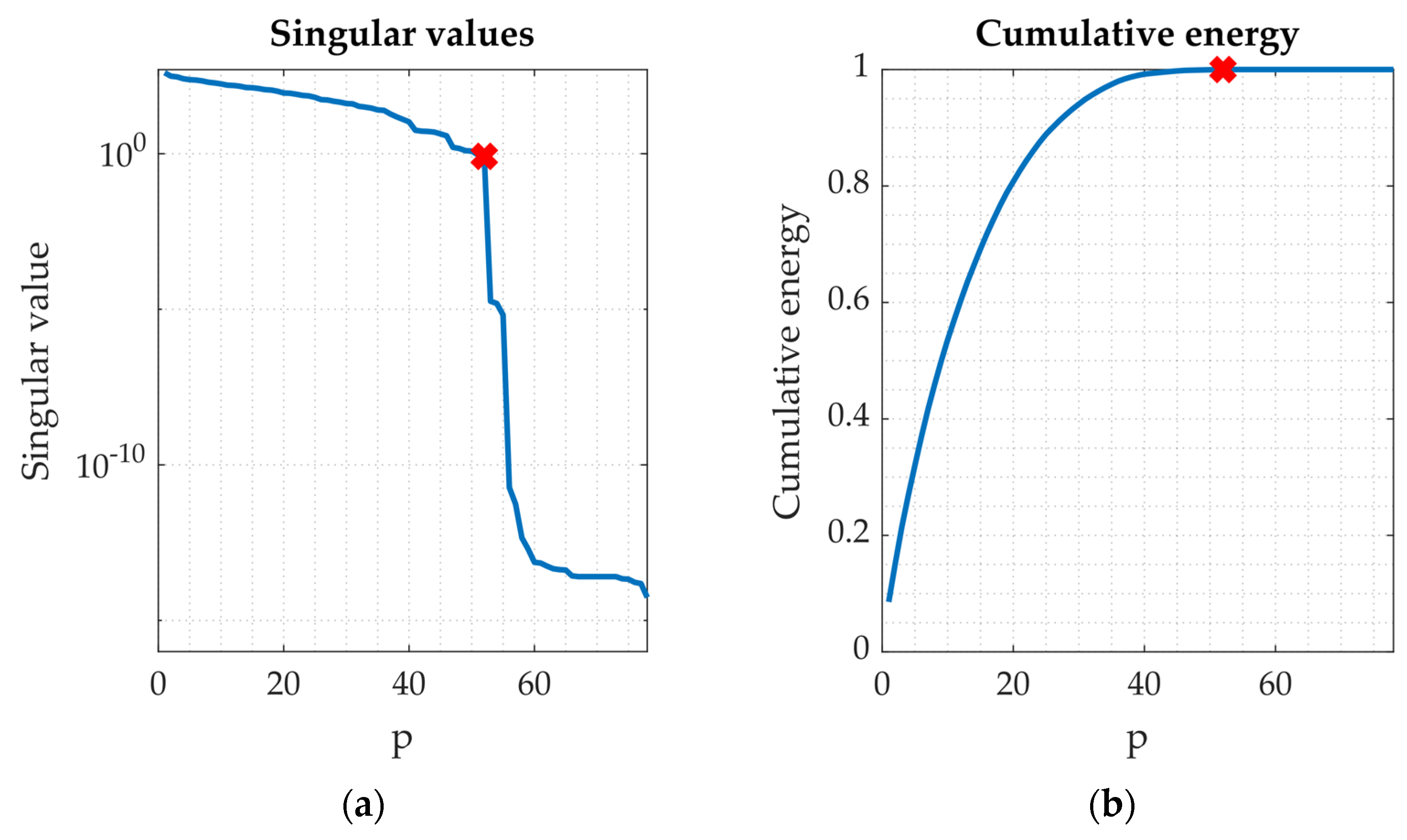
19].
is then written as
, where
is a diagonal matrix, whose non-null elements are the singular values
of
reported in
Figure 1a.
By analyzing the trend of the singular values of
and its cumulative energy [
36] in
Figure 1b, it is possible to see, as also reported in [
29], how 52 base dynamic parameters must be used to fully describe the robot dynamic behavior. If more are adopted, the condition number of
, defined as the ratio between the highest and the lowest singular value
, would drop, jeopardizing the identification process [
37]. A high value of this index, in fact, makes the base dynamic parameters strongly dependent on slight variations of the signals measured from the robot that are affected by noise.
This information is then used to check the quality of the QR decomposition adopted in this work to reduce the system from to and from to . This analysis highlights that not all the 78 dynamic parameters of the manipulator (13 for each joint) can be identified. Indeed, only 30 of them are totally identifiable; 39 are identifiable with linear dependency, while the remaining 9 do not play any role in the dynamics of the manipulator.
On the other hand, when mounting the robot in different configurations (i.e., on a wall, being
and
), the SVD analysis applied to
assesses that the manipulator dynamics is fully described by 54 base dynamic parameters, leading to
. Since the rotation axis of the robot base is not aligned with the gravitational acceleration vector, the mass and two coordinates of the position of the center of mass of the first joint/link need to be identified. So, while the number of the totally identifiable dynamic parameters remains unchanged, 42 of them are now identifiable with linear dependency and only 6 do not affect the robot dynamics. The symbolic equations describing the 54 elements of the vectors
of both the UR3 (
and the UR5 (
are reported in
Appendix A. In the case study in which the robot is positioned on the ground or on the ceiling, the 52 base dynamic parameters are still described by Equations (A1) and (A2), but without the first two rows.
3.2. Optimized Excitation Trajectory
For proper identification of the base dynamic parameters
, a persistent trajectory, built using 5th order Finite Fourier Series (FFS), has been commanded to both the UR3 and the UR5. Angular positions, velocities, and accelerations of each joint
i are calculated according to:
where:
is the fundamental frequency equal for each joint to guarantee the periodicity of the robot’s movement. It is defined as
, where
is the identification trajectory period set to 10 s as in [
29], while similar or lower frequencies have been adopted in [
19,
26,
38];
is the joint position offset equal to [0, −π/2, 0, 0, 0, 0] rad;
and are the coefficients of the FFS that have to be found by optimization to define a trajectory able to continuously excite all the base dynamic parameters.
Since the identification trajectory must be feasible, physical constraints, regarding the maximum joints angular positions (
), velocities (
), and accelerations (
) of the manipulator, were added to the minimization problem. Such values were chosen both according to the mechanical constraints of the robots (
and
are equal to π rad/s and 5.5π rad/s
2, respectively) and to avoid any collision of the robots with themselves or with the external environment by setting
= [2π, π, π, 2π, 2π, 2π] rad. By adapting the equations reported in [
39], these limits have been implemented as:
Moreover, since non-zero values of the joints angular velocities and accelerations would lead to high vibrations at the start and the end of the commanded trajectory, their initial and final values have been set to 0 using:
The FFS coefficients
and
can be identified using different approaches like artificial bee colony [
38], particle swarm [
40], or a Genetic Algorithm (GA) [
18,
41]. In the present work, the MATLAB Global Optimization Toolbox has been used to implement a GA with a population of 300 individuals to minimize the objective function:
where
is the
observation matrix built by piling the single regressors
calculated for each trajectory point
k of the identification trajectory. Other types of cost functions can be found in [
42].
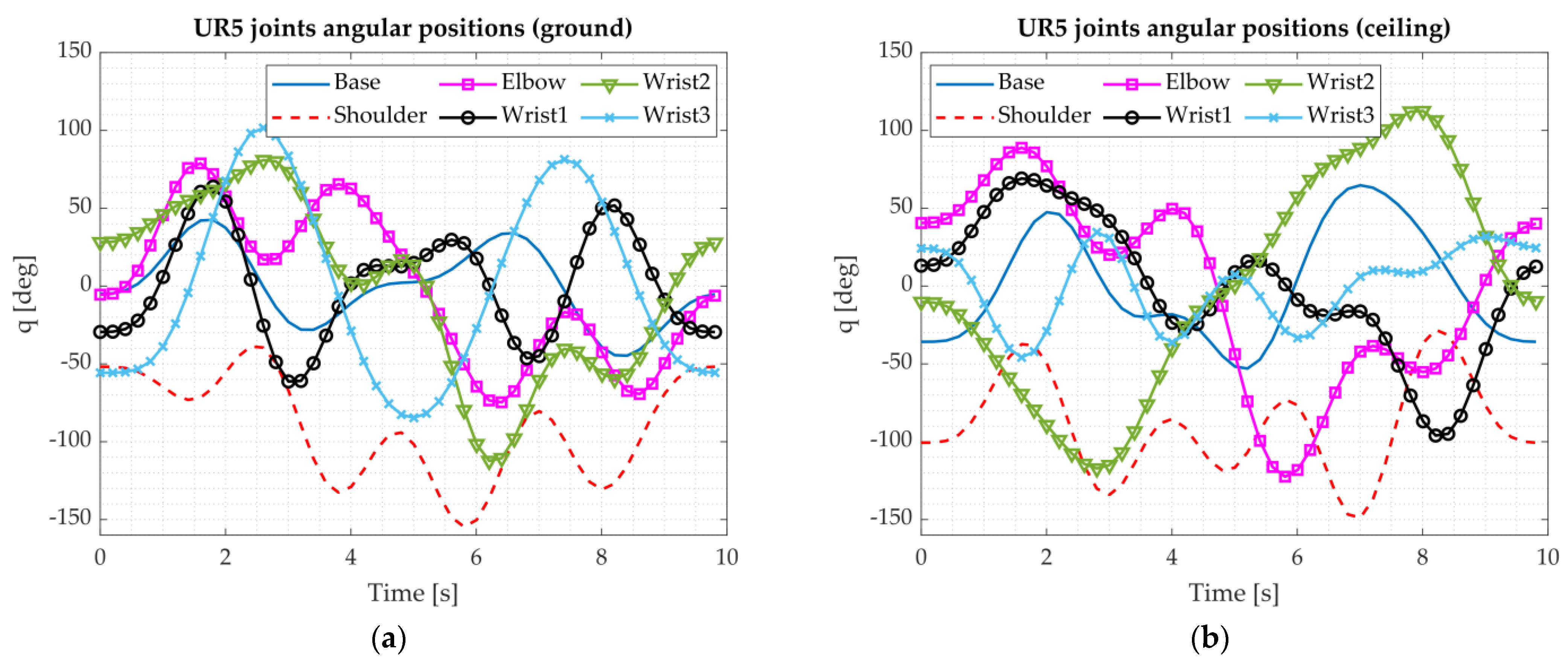
The resulting angular positions obtained for the UR5 collaborative robot are reported in
Figure 2a. Similar values have been also found for the UR3.
A condition number of about half the one related to the trajectory of
Figure 2a has been obtained for the one reported in
Figure 2b in the case the robot would be mounted on the ceiling. This result suggests that more reliable identification of the base dynamic parameters would be obtained by mounting the manipulator on the ceiling rather than on the ground. Nevertheless, as reported in
Section 5, good approximations of the joints torques of both robots have been obtained by calculating their base dynamic parameters while mounted on the ground.
To reduce the risk of an ill-conditioned
, the identified trajectory is repeated three times, leading to a total excitation period of 30 s. To do this, it has been necessary to use the
servoj function created to directly control the joints angular positions and defined as:
servoj(target joint configuration, acceleration, velocity, time, lookahead time, gain) [
43]. Since they are not used in the current version of the robot software, the
acceleration and the
velocity parameters have been set to 0. On the contrary, the
time has been set to 0.008 s being the communication frequency between the robot and the external computer equal to 125 Hz. Experimental tests showed that, for a smooth movement of the robot arm, optimal values for the
lookahead time and the
gain should be 0.03 and 500, respectively. This approach only allows for specifying a set of angular positions to the manipulator, while joints angular velocities and accelerations cannot be directly commanded.
4. Base Dynamic Parameters Identification
As in [
19,
26,
44], to calculate the robots base dynamic parameters
, the Least Squares (LS) algorithm has been adopted as:
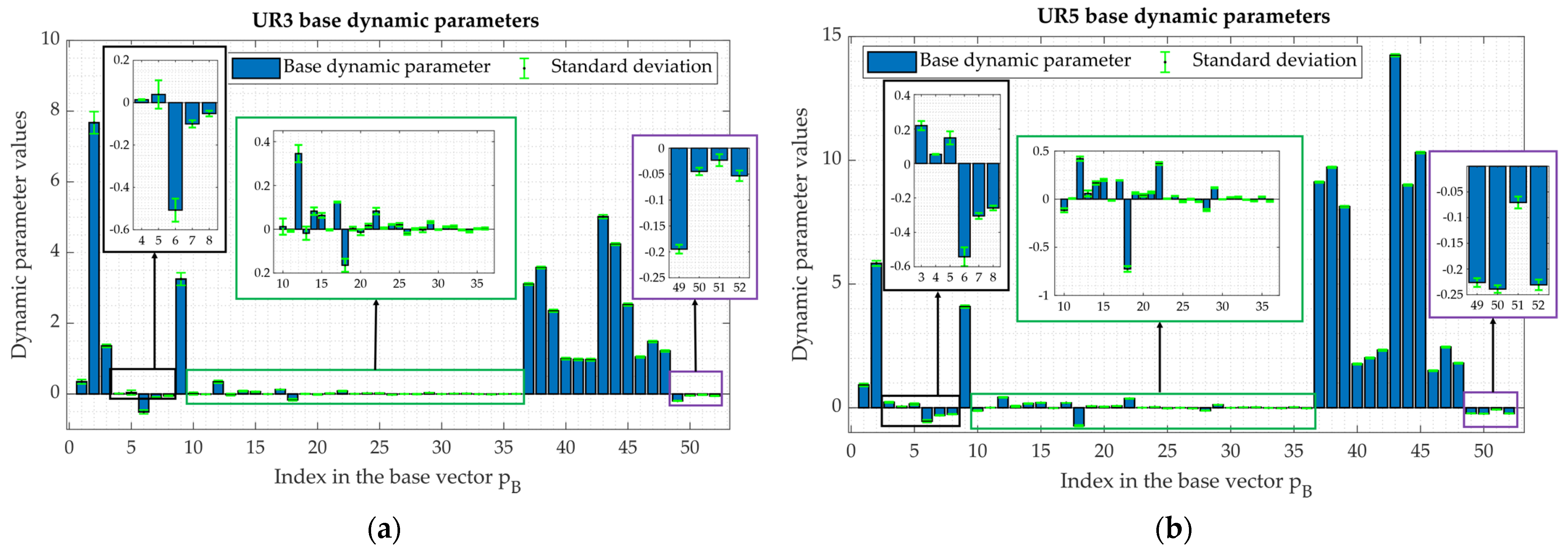
where
is the joints torques vector derived from the motor currents. These values are reported, together with their standard deviations, in
Figure 3a,b for the UR3 and the UR5, respectively. Additional frames have been inserted for better visualization of the small values which cannot be read at full scale.
Since both robots have been mounted on the ground, their dynamic behavior is fully described by 52 base dynamic parameters. In
Figure 3a,b are reported, respectively, the numerical values associated with the elements
and
of the vectors reported in
Equations (A1) and (A2).
Moreover, the standard deviation of each element of has been calculated, resulting in maximum values of 0.313 for the UR3 and 0.107 for the UR5.
An alternative to Equation (9), which takes into account the different sizes of the manipulator joints, is proposed in [
19]. By applying a Weighted Least Squares (WLS) method, the base dynamic parameters are calculated as:
where the coefficients
, for each trajectory point
k, are
with
being the maximum torques of the joint
j, reported in
Table 2.
In the proposed application, the LS method has been preferred to the WLS one for two main reasons:
A third approach is described in [
46], where a Constrained Weighted Least Squares (CWLS) method has been implemented using the constraints associated with links masses and inertia tensors reported in [
47]. This ensures a positive definite mass matrix for each trajectory point
k. If such condition is not satisfied, the algorithm provides physically impossible results, such as the negative motors inertia (
) of the last four joints of both manipulators. Although more accurate, this method requires a global optimization algorithm to calculate the base dynamic parameters, hence resulting in a far more time-consuming procedure than the LS and WLS. Alternative approaches can be found in [
48], where an extensive review of the most used algorithms for dynamic parameters calculation is reported.
Besides, since both Coulomb (
) and viscous friction (
) coefficients are fully identifiable, it would be possible to use the proposed identification algorithm to estimate the health status of all the manipulator joints. An increment of the friction parameters, for example, could be related to a higher level of wear in the joint bearings and gearbox. Even though it would not be possible to locate the root cause of the fault, this information could be used, together with other health features extracted from the robot signals, to estimate the overall operating condition of the machine and its remaining useful life. The reliability of the identified friction coefficients is also highlighted by the similar values of
and
and of
and
of the UR3 and the UR5, respectively. Since, as reported in
Table 2, the joints mounted at the UR3 elbow and the UR5 wrists are the same, also their Coulomb and viscous friction coefficients are similar.
The values reported in
Figure 3a,b have been calculated for the robot arm only. In the case a tool is mounted, the identified dynamic parameters must be updated to allow the model to correctly estimate the joints torques. To do so, it would be only necessary to execute again the excitation trajectory and apply the LS method reported in Equation (9). A tool, in fact, can be considered as an extension of the robot last link and it does not add any additional degree of freedom to the manipulator, so the regression matrix does not change. On the other hand, in the case of a cumbersome tool, it could be necessary to find another persistent trajectory for the identification process since some changes to the robot constraints
could be required to avoid possible collisions.
5. Validation of the Identified Base Dynamic Parameters
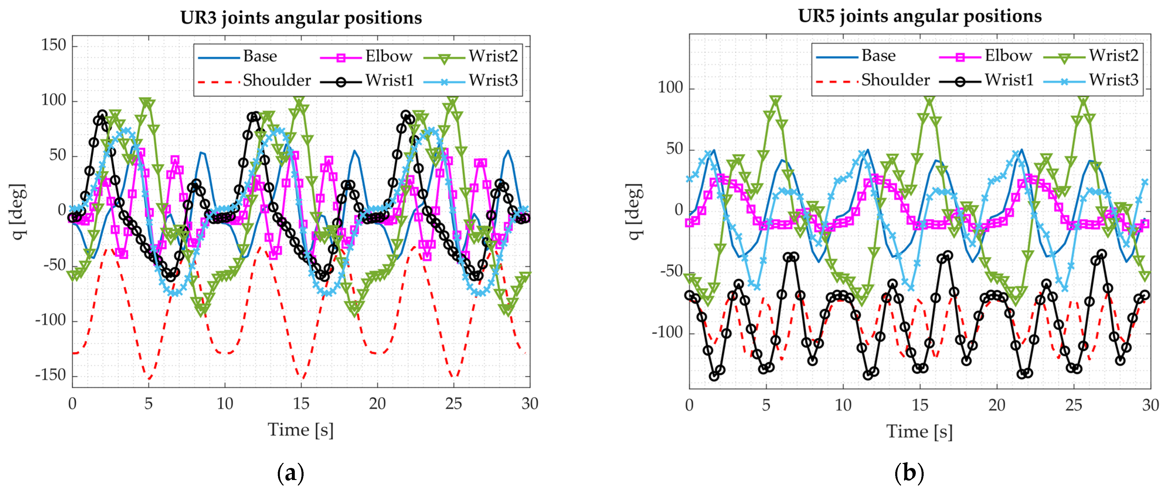
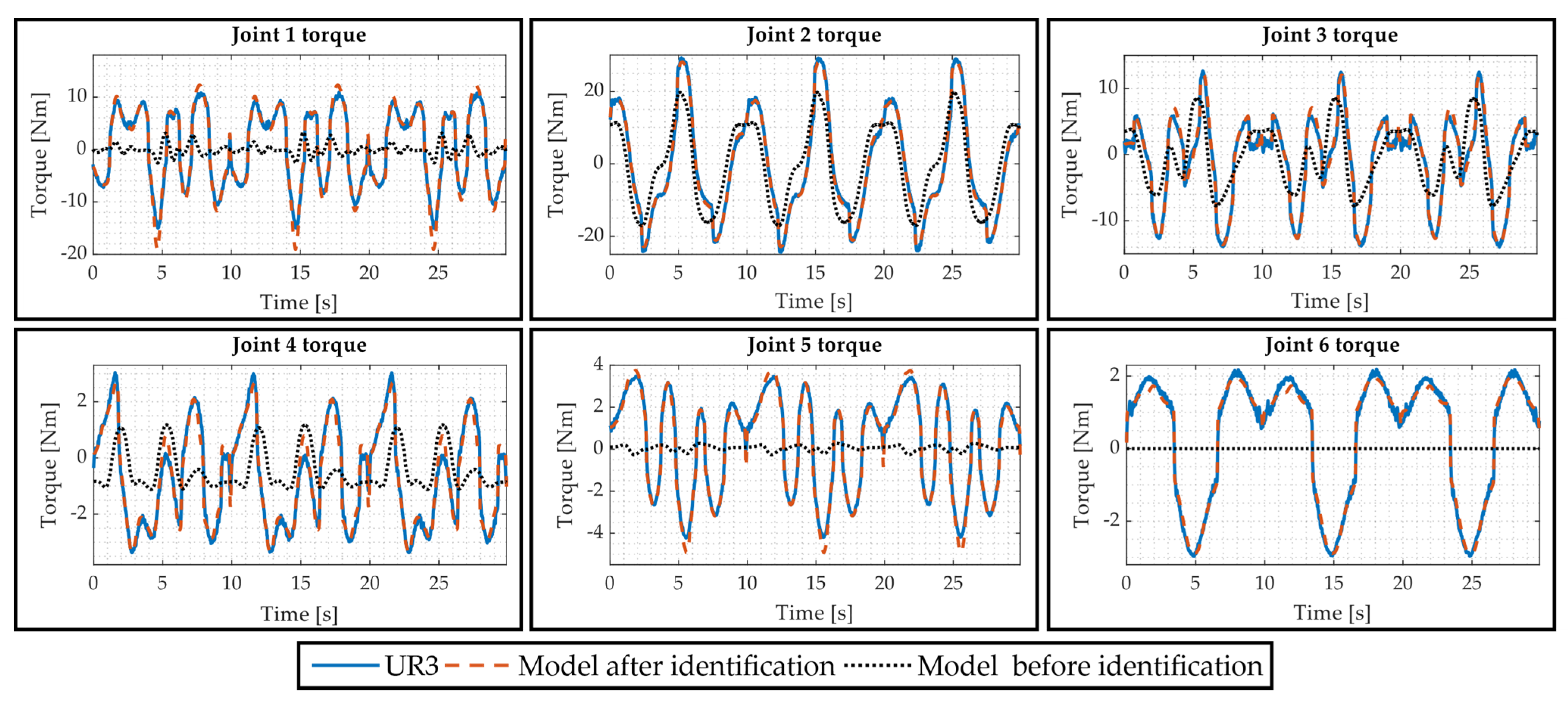
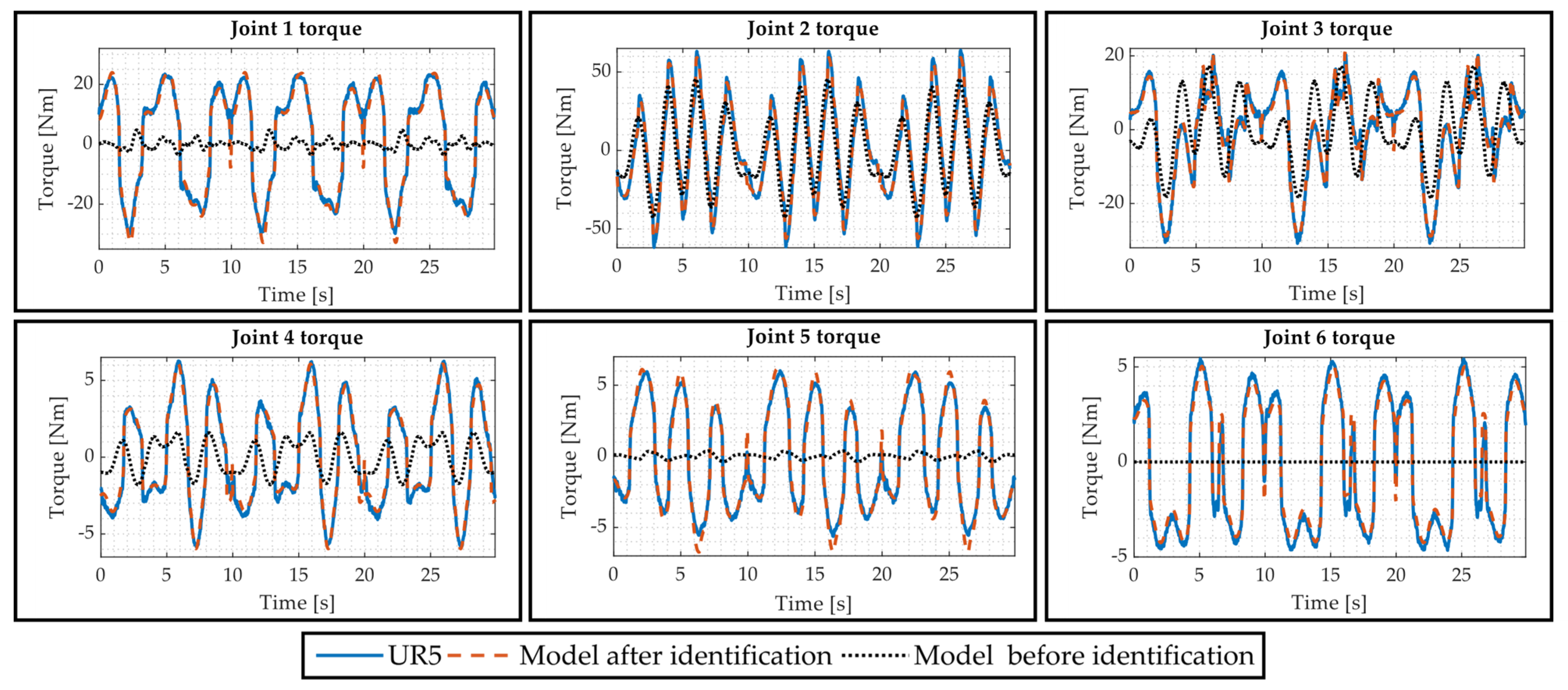
The validation of the proposed algorithm has been done by commanding the two robots with several persistent trajectories, like the ones reported in
Figure 4a,b. These have been obtained by substituting pseudo-random values to the FFS coefficients
ai,l and
bi,l in Equation (5) so that the boundary conditions of Equations (6) and (7) are respected. This approach allows defining persistent trajectories able to excite all the identified base dynamic parameters reported in
Appendix A. The corresponding joints torques of the UR3 and the UR5 are reported in
Figure 5 and
Figure 6, respectively.
To evaluate the accuracy of the identified base dynamic parameters, in
Figure 5 and
Figure 6 the measured torques (UR3 and UR5, respectively) are compared with the ones estimated with the proposed mathematical model once that the base dynamic parameters
have been identified (Model after identification). In addition, the joints torques (Model before identification), obtained using only the dynamic parameters provided by the manufacturer [
1], are also reported.
This analysis highlights how a proper identification of the robot dynamic parameters is crucial for a correct estimate of the joints torques of a manipulator. As in [
26], the normalized error, defined as
, is adopted to better quantify the mismatch among measured and modeled joint torques. In the present study, the error vector
has been calculated in three different ways:
, where
and
are the measured torques for each point
k of the validation trajectory and the ones obtained using only the dynamic parameters found in [
1];
, with being the observation matrix calculated for the validation trajectory;
, where, instead of the base dynamic parameters , the ones obtained through the WLS method have been used.
For the validation trajectories depicted in
Figure 4a,b, the normalized errors are reported in
Table 3.
By both comparing the trends of the measured and the estimated torques of
Figure 5 and
Figure 6 and the values of the normalized errors of
Table 3, the validation process has been considered to be successful.
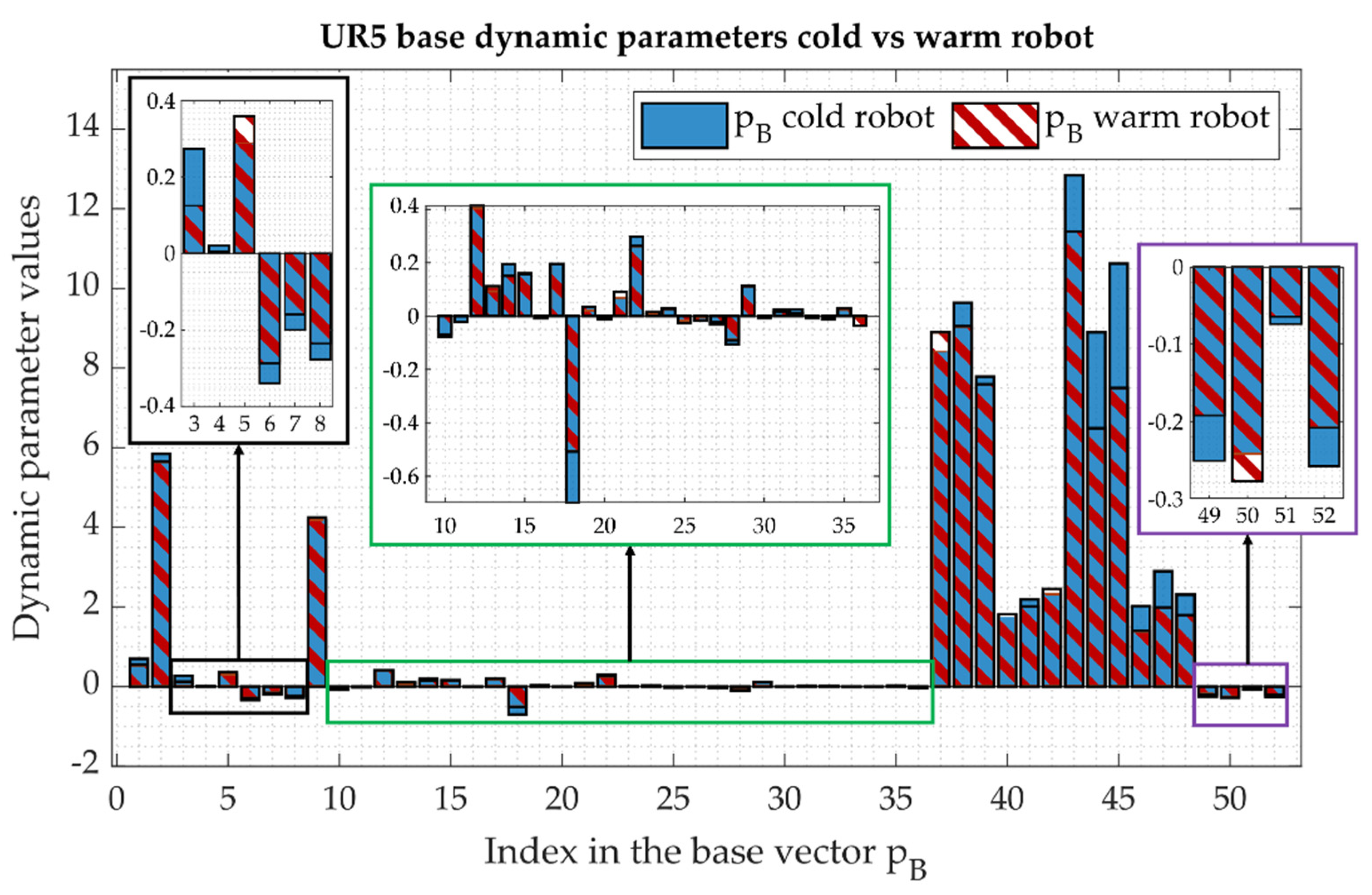
6. Temperature Effect on the Base Dynamic Parameters
For a proper modeling and control strategy of a manipulator, the effect of temperature on the robot dynamics should be taken into account. To better show its impact on the base dynamic parameters, the identification trajectory of
Figure 2a has been commanded to the UR5 just after its power-up (cold robot) and after half an hour warm-up (warm robot). Joints temperatures have been measured by built-in robot sensors and acquired at 125 Hz via TCP/IP communication using port 30003. Their mean values are hereby reported:
Cold robot: T = [25.2, 24.9, 22.2, 26.1, 22.4, 23.2] °C;
Warm robot: T = [36.5, 34.6, 32.6, 37.9, 39.7, 40.1] °C.
The identified base dynamic parameters are depicted in
Figure 7, where additional frames have been inserted for better visualization of the small values which cannot be read at full scale.
The values (
) and (
), which should not depend on temperature, are nearly the same in both working conditions, proving the stability of the algorithm. On the other hand, there are differences in the friction parameters (
), with a reduction of up to 31% of the viscous ones. Similar percentual variations have been also observed in [
19,
49].
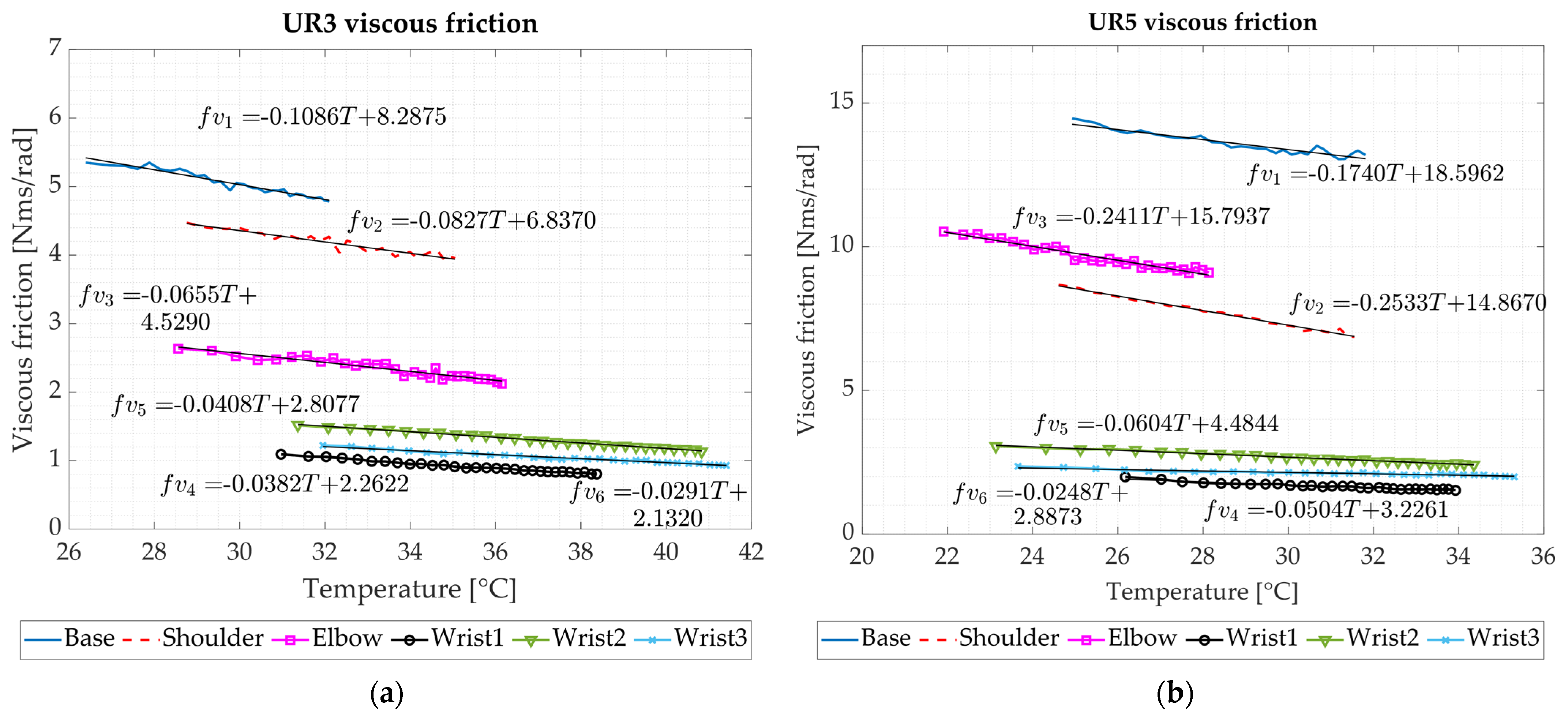
Since viscous friction depends on joints temperature, a more detailed analysis to better quantify such a correlation has been carried out with both the UR3 and the UR5. To do so, the identification process of the base dynamic parameters has been sequentially repeated multiple times for both manipulators by commanding the same persistent trajectory of
Figure 2a. The results are reported in
Figure 8a,b.
Since an increment of the joint temperature reduces the viscosity of the grease used to lubricate the joints, the values of the viscous friction coefficients linearly decrease with the rise of temperature in the considered range. The overall percentage reductions of the viscous friction coefficients, between the initial and the final robot operating conditions, are reported in
Table 4.
This analysis also highlights the different operating conditions of the two robots even if commanded with the same persistent trajectory. By considering the temperature ranges in
Figure 8a,b, it can be seen how, because of their different heat dissipation properties, smaller joints tend to reach higher temperatures than the bigger ones. So, since grease viscosity and joint temperature are inversely proportional in the considered temperature range, this also explains why the viscous friction coefficients of the UR3 face, on average, higher percentage reductions than the ones of the UR5.
Moreover, by comparing the curves related to the UR3 elbow and the three UR5 wrist joints, which are the same, it is possible to observe how the four trends are comparable although different. The slight variations among the three wrist joints of the UR5 could be caused by their possible different lubrication conditions. On the other hand, since the UR3 has been operative for longer than the UR5, their mismatch with the UR3 elbow joint may be related to wear [
50]. However, since the manufacturer does not provide any information related to the single joint usage, this assumption, although plausible, cannot be confirmed.
Moreover, to better highlight the impact of changes in grease viscosity on the joints torques necessary to execute the persistent trajectory of
Figure 2a, their average and maximum differences, between the initial and the final operating conditions of both manipulators, have been reported in
Table 5 and
Table 6.
Even though the average variations of
Table 5 could be neglected, it should be pointed out that viscous friction torques directly depend on joints angular velocities, so the values reported in this study would be different for other trajectories. This dependency is particularly relevant for industrial robots which usually reach high speeds to maximize productivity. However, by analyzing the values reported in
Table 6, it becomes clear how temperature variations affect the dynamic behavior of the tested robots. Such a dependency of joints friction on temperature is also highlighted when comparing the values of
Table 6 with the maximum torques, listed in
Table 2, that the single joints can provide. The weighted percentage variations, reported as an average among all the joints of the same size belonging to the same robot, are reported in
Table 7.
Future studies will be devoted to mapping the dependency of the robot viscous friction coefficients with temperature in the entire working range 0–50 °C defined by Universal Robots.
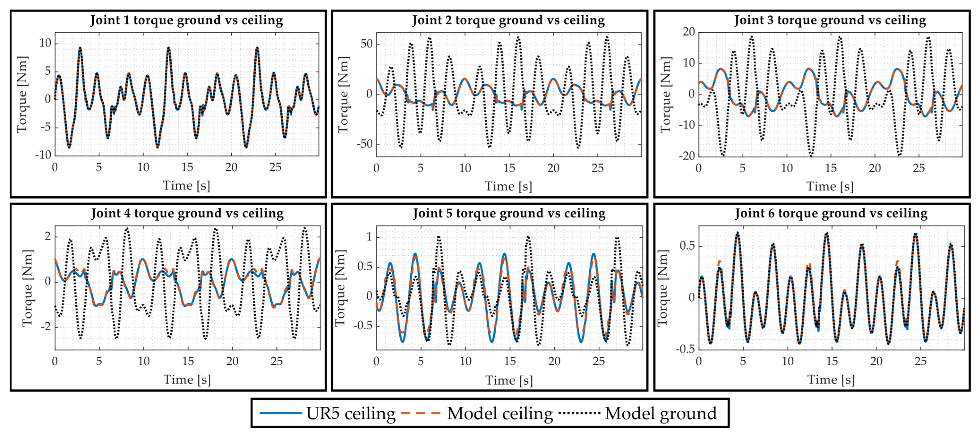
7. Mounting Configuration Effect on Joints Torques Estimate
To prove the adaptability and reliability of the proposed mathematical model, URSim has been adopted to estimate the torques of the digital twin of a UR5 mounted on the ceiling using the same validation trajectory depicted in
Figure 4b. Despite the case in which a tool is added, since the system under analysis is only composed of the UR5, the base dynamic parameters are the same as the ones identified when the manipulator is positioned on the ground. On the contrary, the regressor
is a function of the robot mounting configuration, so it must be recalculated. If not, there would be a mismatch among the estimated and the measured joints torques since URSim and the proposed mathematical model would describe two different physical systems. As reported in
Figure 9, by updating the regression matrix, the estimated torques (Model ceiling) well approximate the ones measured from URSim (UR5 ceiling). On the contrary, if the same regressor obtained for the robot mounted on the ground would have been used, the predicted torques (Model ground) would have not correctly describe the dynamic behavior of the system under analysis, as also proved by the high value of the normalized error
reported in
Table 7.
This can be also seen by calculating the joints torques errors, and the corresponding normalized errors reported in
Table 8, of the simulated robot in three different scenarios:
, where are the torques read from URSim for each point of the validation trajectory in the case the robot is mounted on the ground, while are the predicted ones obtained using the base dynamic parameters identified through Equation (9) using the data from URSim;
, where the acquired () and the predicted torques () have been calculated as in the previous point, but in the case of the robot mounted on the ceiling;
, where the two mounting configurations are compared to emphasize the high errors that would have been made if the robot mounting configuration would have not been taken into account.
By comparing the normalized error for the UR5 obtained after the identification of its base dynamic parameters using the LS method (
Table 3) with the one in
Table 8 for the simulated robot in the same operating conditions (
), it can be seen that the first one is higher than the second one. This is related to the fact that there is no noise in the signals coming from the simulated robot, so the negative effect of the regressor condition number is limited. So, the main advantage of testing both the identification and the validation processes with URSim is that the quality of the manipulator base dynamic parameters and, as a consequence, the one of the predicted torques, is higher than the one obtained using the real robot. The stability of the identification process and the ability of the model to effectively predict joints torques in different mounting configurations are also confirmed by the low value of
, which is comparable with the one obtained when the robot is mounted on the ground.
It is also worth noting that, in the case of the UR5 mounted on the ground, the estimated torques (Model ground) and the ones reported in
Figure 6 are not equal. This difference is related to the fact that URSim does not take into account link inertia and joints friction. This proves that the official offline simulator developed by the robot manufacturer cannot be effectively used for an accurate estimate of the dynamic behavior of the manipulator.
8. Conclusions
The present paper highlights how changes in the robot operating conditions affect its dynamic behavior. To do so, a mathematical model able to identify the dynamic parameters of an industrial manipulator is presented and validated with the collaborative robots UR3 and UR5. The two manipulators have been both commanded with persistent exciting trajectories based on 5th order finite Fourier series optimized using a genetic algorithm. Based on the data sampled during the experimental campaign, after the identification of the robots’ base dynamic parameters, the normalized error among the measured and the simulated joints torques is reduced by about the 90% with respect to the one obtained with only the manipulators dynamic properties provided by Universal Robots.
The identification process has been then used to investigate and quantify the effects of temperature on joints viscous friction parameters, allowing a more reliable estimate of the joints torques of the real robot in different working conditions. In the considered temperature range, experimental data showed a reduction of the viscous friction coefficients of about 20% and 17% for the UR3 and the UR5, respectively. This leads to a variation of the joints torques of up to about 8% of the maximum ones transmissible from the robots, showing how this dependency cannot be neglected in the definition of a high-fidelity model of an industrial manipulator.
Due to the possibility to fully identify both Coulomb and viscous friction coefficients and their strict relation with wear, future tests will be run to evaluate the implementation of the proposed algorithm to estimate the health status of the manipulator joints.
In addition, the proposed model has been developed to take into account different mounting configurations which affect the number of base dynamic parameters necessary to fully describe the robot dynamic behavior. The adaptability of the identification algorithm to different setups has been validated using the official simulator developed by the same manufacturer of the tested robots.
The next steps will be focused on testing the proposed algorithm on other robots mounted in different configurations. Moreover, since this work is part of a larger research project whose goal is the definition of a high-fidelity model of an industrial manipulator, more accurate and physically reliable dynamic parameters are required. To do so, the least square method used for the identification process will be replaced with a global optimization algorithm. This would allow building a digital twin of a specific machine in which diagnostics and prognostics algorithms will be implemented to study the fault to failure mechanisms in an industrial robot and their effects on its behavior.


 ,
, 


