Plane Symmetric Cosmological Model with Strange Quark Matter in f(R,T) Gravity

Abstract

A plane symmetric Bianchi-I model filled with strange quark matter (SQM) was explored in $f(R,T)=R+2\lambda T$ gravity, where R is the Ricci scalar, T is the trace of the energy-momentum tensor, and $\lambda$ is an arbitrary constant. Three different types of solutions were obtained. In each model, comparisons of the outcomes in $f(R,T)$ gravity and bag constant were made to comprehend their roles. The first power-law solution was obtained by assuming that the expansion scalar is proportional to the shear scalar. This solution was compared with a similar one obtained earlier. The second solution was derived by assuming a constant deceleration parameter q. This led to two solutions: one power-law and the other exponential. Just as in the case of general relativity, we can obtain solutions for each of the different eras of the universe, but we cannot obtain a model which shows transitional behavior from deceleration to acceleration. However, the third solution is a hybrid solution, which shows the required transition. The models start off with anisotropy, but are shear free at late times. In general relativity, the effect of SQM is to accelerate the universe, so we expect the same in $f(R,T)$ gravity.

1. Introduction

Observational data [1,2,3] suggest that the universe is currently in an accelerating epoch. A plethora of attempts have been made to explain this phenomenon, but none of them is compelling. The first attempt is “Dark energy” (DE), which is the hypothesis of exotic matter with the unique feature of anti-gravity due to its negative pressure, albeit small, thereby accelerating the universe [4]. The cosmological constant (CC) is the primary candidate for DE [5]. However, the shortcomings of the $\mathsf{\Lambda }CDM$ model [6] enable researchers to consider other alternatives to the CC. There are variable DE candidates, e.g., quintessence [7] and phantom energy [8,9]. An alternative approach to explain the acceleration of the universe is modified theories of gravity, e.g., higher derivative theories, Gauss–Bonnet $f\left(G\right)$ gravity, $f\left(R\right)$ theory, and $f\left(T\right)$ and $f(R,T)$ gravity theories (for a detailed review, see [10]). In 2011, Harko et al. [11] introduced $f(R,T)$ gravity, where $f(R,T)$ is an arbitrary function of the Ricci scalar R, and the trace T of the energy-momentum tensor. A noticeable feature of this theory is the presence of acceleration due to the coupling between matter and spacetime geometry. This phenomenon produces significant signatures and effects, which distinguishes it from other theories of gravity. The theory is compatible with spacetime symmetries (for details, see ref. [12]). In addition, it does not have ghosts or Laplacian instabilities [13]. The theory has also been tested on galactic and intra-galactic scales [14,15,16,17], etc. Therefore, this theory has caught the attention of many researchers for the study of various cosmological and astrophysical phenomena (see [18] for an extensive list of references).

Most of the early studies were focused on a spatially flat homogeneous and isotropic universe, well articulated by the Friedmann–Lemaitre–Robertson–Walker (FLRW) metric. Due to anisotropy at small scales supported by both observational and theoretical data [19,20], several authors have also considered an anisotropic background (see [21,22] and the references therein). The Bianchi type-I (B-I) model is one of the favored spacetimes to study the effects of early-time anisotropy since it is a basic generalization of the FLRW $k=0$ model.

In order to comprehend the early stages of the evolution of the universe, it is important to study quark gluon plasma (QGP). It is understood that two phase transitions occurred in the very early universe as it cooled down, namely, the quark gluon phase and the quark hadron phase. During the first few seconds after the big-bang, a phase known as the quark gluon phase occurred, where quark matter (QM) is thought to have originated. The second phase occurred at a temperature of $T=$ 200 MeV due to adiabatic expansion of the universe, when the QGP was transformed into a hadron gas [23,24,25]. Later on, many authors [26,27,28,29,30] proposed the theoretical possibility of strange quark matter (SQM) constituting the ground state of hadronic matter, which implies that neutron stars could become strange stars. Though SQM has not yet been confirmed, the properties and possibilities of locating it have been extensively explored by many researchers [31,32,33,34,35,36,37,38,39,40,41].

There are many aspects of QGP, QM, and SQM that have been investigated, e.g., SQM in the Godel universe [42], inflation with SQM at the quantum chromodynamics (QCD) phase transition [43], the spacetime structure of the first few seconds after the big bang when QGP may exist [44], QM as DE and dark matter (DM) at galactic scales [45], and thermodynamics and the geometry of SQM [46]. Many authors have studied cosmological models containing QM and SQM in 5-D Kaluza–Klein spacetime [47], higher dimensional spacetimes [48,49,50], self-creation cosmology [51,52] and Brans–Dicke theory [53]. Some authors have considered axially symmetric anisotropic cosmological models [54,55]. Yilmaz [56] studied B-I and B-V cosmological models with QM and SQM in $f\left(R\right)$ gravity.

Recently, Singh and Beesham [57] studied a locally rotationally symmetric (LRS) B-I model with SQM and a time-dependent cosmological term in $f(R,T)$ gravity and found that SQM could be a possible candidate of DE. Agrawal and Pawar [58] considered a plane-symmetric B-I model with SQM; however, the field equations obtained by those authors were incorrect. Also, the authors over determined the solutions. In this paper, we explored the model considered in ref. [58] and extend the solutions by considering three different models, namely, the constant deceleration parameter model describing a decelerated universe, a model with special law of Hubble parameter, which can describe a decelerated as well as an accelerated universe, and a model exhibiting a transition from a decelerated to an accelerated universe.

The work is organized as follows. The formalism of $f(R,T)$ gravity theory is presented in Section 2. Considering a specific form of $f(R,T)=R+2\lambda T$ in the presence of SQM, the field equations for plane-symmetric spacetime are obtained in Section 3. In Section 4, the solutions are obtained by considering the expansion scalar to be proportional to the shear scalar. In Section 5, a special law of the Hubble parameter is considered to find the solutions. A transit model by assuming a hybrid scale factor is considered in Section 6. The findings of each model are summarized in the concluding Section 7.

2. The Formalism of $\mathit{f}(\mathit{R},\mathit{T})$ Gravity Theory

The general action of $f(R,T)$ gravity with units $8\pi G=1=c$ is given by [11]

$$S=\frac{1}{2}\int \left[f(R,T)+2L_m\right]\sqrt{-g}{d}^{4}x,$$

(1)

where $f(R,T)$ is an arbitrary function of the scalar curvature R, and the trace T of the energy-momentum tensor (EMT), $L_m$ is the matter Lagrangian density, and g is the determinant of the metric tensor $g_{ij}$.

The EMT is defined by

$$T_{ij}=-\frac{2}{\sqrt{-g}}\frac{\delta \left(\sqrt{-g}{L}_m\right)}{\delta g^{ij}},$$

(2)

Since $L_m$ depends on the metric tensor $g_{ij}$ rather than its derivatives, (2) becomes

$$T_{ij}=g_{ij}{L}_m-2\frac{\partial L_m}{\partial g^{ij}}.$$

(3)

Varying (1) with respect to $g_{ij}$, one obtains the field equations for $f(R,T)$ gravity

$$f_R{R}_{ij}-\frac{1}{2}f(R,T)g_{ij}+\left(g_{ij}\square -{\nabla }_i{\nabla }_j\right)f_R=T_{ij}-f_T{T}_{ij}-f_T{\mathsf{\Theta }}_{ij},$$

(4)

where $f_R$ and $f_T$ represent the partial derivatives of $f(R,T)$ with respect to R and T, respectively, ${\nabla }_i$ is the covariant derivative, $\square \equiv {\nabla }_{\delta }{\nabla }^{\delta }$ is the d’Alembertian operator, and ${\mathsf{\Theta }}_{ij}$ is defined as

$${\mathsf{\Theta }}_{ij}\equiv g^{\mu \nu }\frac{\delta T_{\mu \nu }}{\delta g^{ij}}.$$

(5)

Substituting (3) in (5) results in

$${\mathsf{\Theta }}_{ij}=-2T_{ij}+g_{ij}{L}_m-2g^{\mu \nu }\frac{{\partial }^2{L}_m}{\partial g^{ij}\partial g^{\mu \nu }}.$$

(6)

Since the field equations in $f(R,T)$ depend on ${\mathsf{\Theta }}_{ij}$, an array of models depending on the nature of the matter source can be generated. This is analogous to choosing various forms of $f(R,T)$. However, the equations in $f(R,T)$ gravity are much more complicated even for the FLRW metric as compared to GR. Therefore, it is very difficult working with a general form of $f(R,T)$ or to solve the field equations in general. Therefore, most of the works in $f(R,T)$ gravity have been carried out by assuming a number of suitable forms of $f(R,T)$, such as $f(R,T)=R+2f\left(T\right)$, $f(R,T)=Rf\left(T\right)$, $f(R,T)={\lambda }_3{f}_1\left(R\right)+{\lambda }_4{f}_2\left(T\right)$, where $f_1\left(R\right)$ and $f_2\left(T\right)$ are arbitrary functions of R and T, and ${\lambda }_3$ and ${\lambda }_4$ are real constants, respectively (see [59] and the references therein). In this work, we study $f(R,T)$ gravity in the form [11]

$$f(R,T)=R+2f\left(T\right),$$

(7)

for which (4) becomes

$$R_{ij}-\frac{1}{2}R{g}_{ij}=T_{ij}-2(T_{ij}+{\mathsf{\Theta }}_{ij})f^{\prime }\left(T\right)+f\left(T\right)g_{ij},$$

(8)

where a prime represents an ordinary derivative of $f\left(T\right)$ with respect to T.

3. The Model and Field Equations

The spatially homogeneous and anisotropic LRS B-I spacetime metric is given by

$$d{s}^2=d{t}^2-A^2(d{x}^2+d{y}^2)-B^{2}d{z}^2,$$

(9)

where A and B are the scale factors and are functions of the cosmic time t. The average scale factor is defined as

$$\begin{array}{ccc}\hfill a& =& {\left(A^{2}B\right)}^{\frac{1}{3}}.\hfill \end{array}$$

(10)

The rates of expansion along the x, y, and z-axes are defined as

$$H_1=\frac{\dot{A}}{A}=H_2,H_3=\frac{\dot{B}}{B},$$

(11)

where a dot represents a derivative with respect to t. The average expansion rate, which is the generalization of the Hubble parameter in an isotropic scenario, is given by

$$H=\frac{1}{3}\left(\frac{2\dot{A}}{A}+\frac{\dot{B}}{B}\right).$$

(12)

The expansion scalar, $\theta$, and the shear scalar, ${\sigma }^2$, are, respectively, defined as

$$\theta =u^i{\nabla }_i=3H,$$

(13)

$${\sigma }^2=\frac{1}{2}{\sigma }_{ij}{\sigma }^{ij}=\frac{1}{3}{\left(\frac{\dot{A}}{A}-\frac{\dot{B}}{B}\right)}^2,$$

(14)

where $u^i$ is the four-velocity of the fluid.

Since QGP behaves similarly to a perfect fluid [60,61], the EMT of SQM is given by

$$T_{ij}=({\rho }_{sq}+p_{sq})u_i{u}_j-p_{sq}{g}_{ij},$$

(15)

where ${\rho }_{sq}$ is the energy density and $p_{sq}$ the thermodynamic pressure of the SQM. In co-moving coordinates, $u^i={\delta }_0^i$, where $u_i$ is the four-velocity of the fluid that satisfies the condition $u_i{u}^i=1$.

The trace $T=g^{ij}{T}_{ij}$ of (15) gives

$$T={\rho }_{sq}-3p_{sq}.$$

(16)

In a bag model [62],

$${\rho }_{sq}={\rho }_q+B_c,$$

(17)

$$p_{sq}=p_q-B_c,$$

(18)

where ${\rho }_q$, $p_q$ are the energy density and pressure of the QM, respectively, and $B_c$ is the bag constant. With the assumption that quarks are non-interacting and massless particles, their pressure is approximated by an equation of state (EoS)

$$p_q=\frac{{\rho }_q}{3}.$$

(19)

The SQM follows an EoS $p_{sq}=\frac{1}{3}\left({\rho }_{sq}-{\rho }_0\right)$, where ${\rho }_0$ is the energy density at zero pressure. In a bag model ${\rho }_0=4B_c$, hence

$$p_{sq}=\frac{{\rho }_{sq}-4B_c}{3}.$$

(20)

The matter Lagrangian is not distinctive. Hence, to be consistent with the variation of the EMT (15) with respect to $g_{ij}$, the assumption $L_m=-p_{sq}$ is used. Consequently, not only the theory becomes compatible with spacetime symmetry, but the second-order variation of the matter Lagrangian in (6) also vanishes, and ${\mathsf{\Theta }}_{ij}$ becomes

$${\mathsf{\Theta }}_{ij}=-2T_{ij}-p_{sq}{g}_{ij}.$$

(21)

Now, the question that arises is whether isotropy is compatible with SQM. This question has been studied in detail by Yilmaz and Aktas [12], who studied a general setting for SQM and concluded that isotropy is indeed compatible with SQM. This is also borne out by several experiments [60,61].

Since the choice of the matter Lagrangian $L_m=-p_{sq}$ is not unique for a perfect fluid, Moraes [63] has eliminated this arbitrariness by deriving the following matter Lagrangian:

$$L=\left[T+\frac{dT}{dF}(R+T+2F)\right]$$

where F is a function of T only. The choice above eliminates the need for choosing a particular matter Lagrangian density.

Inserting (21) into (8), one obtains

$$R_{ij}-\frac{1}{2}R{g}_{ij}=\left[1+2f^{\prime }\left(T\right)\right]T_{ij}+\left[2p_{sq}{f}^{\prime }\left(T\right)+f\left(T\right)\right]g_{ij}.$$

(22)

The structure of $f(R,T)$ gravity is such that there are many choices for the function $f(R,T)$, each of which leads to a different set of models. The main aim of this paper was to study the effects of SQM in $f(R,T)$ gravity, and so we chose the simplest parametrization of $f(R,T)$, i.e., $f(R,T)=R+2f\left(T\right)=R+\lambda T$, where $\lambda$ is an arbitrary constant. The simplest non-minimal matter–geometry coupling within $f(R,T)$ gravity is given by $f(R,T)=R+\lambda RT$ (see, e.g., [64]). However, to study SQM in such a coupling would be tantamount to writing another paper, and this is beyond the scope of the present analysis.

From (16)–(20), we have $T=4B_c$, which is a constant. Consequently, $f\left(T\right)=4\lambda B_c$, which implies $f^{\prime }\left(T\right)=0$. Hence, (22) reduces to

$$R_{ij}-\frac{1}{2}R{g}_{ij}=T_{ij}+4\lambda B_c{g}_{ij}.$$

(23)

Assuming, $4\lambda B_c=\mathsf{\Lambda }$, the above field equations become equivalent to Einstein’s field equations with a cosmological constant. Then, $f(R,T)=R+2\lambda T$ becomes $f(R,T)=R+8\lambda B_c$. Hence, $f(R,T)=R+2\lambda T$ for $f\left(T\right)=\lambda T$ with SQM is equivalent to the $\mathsf{\Lambda }$CDM ($\mathsf{\Lambda }$ cold dark matter) model. Interestingly, while a cosmological constant is added to Einstein’s field equations ad hoc, here it results naturally from the coupling of $f(R,T)$ gravity and the bag constant. If $\lambda =0$ or $B_c=0$, (23) reduces to the field equations in GR.

The field Equations (23) for the Metric (9) and EMT (15), yield

$$\begin{array}{ccc}\hfill {\left(\frac{\dot{A}}{A}\right)}^2+2\frac{\dot{A}\dot{B}}{AB}& =& \left({\rho }_q+B_c\right)+4\lambda B_c,\hfill \end{array}$$

(24)

$$\begin{array}{ccc}\hfill {\left(\frac{\dot{A}}{A}\right)}^2+2\frac{\ddot{A}}{A}& =& -\left(p_q-B_c\right)+4\lambda B_c,\hfill \end{array}$$

(25)

$$\begin{array}{ccc}\hfill \frac{\ddot{A}}{A}+\frac{\ddot{B}}{B}+\frac{\dot{A}\dot{B}}{AB}& =& -\left(p_q-B_c\right)+4\lambda B_c.\hfill \end{array}$$

(26)

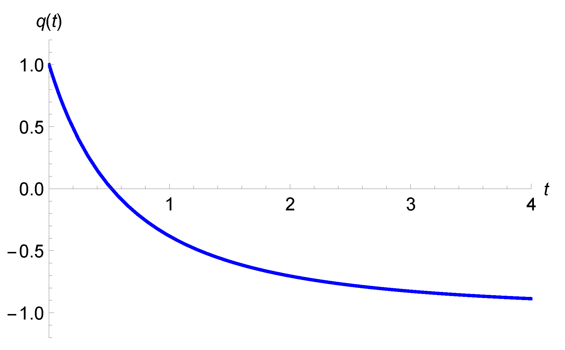
4. Model I: Expansion Scalar Proportional to the Shear Scalar

Equations (24)–(26) are three independent equations consisting of four unknowns, namely, A, B, $p_q$, and ${\rho }_q$. Therefore, in order to find exact solutions, one supplementary constraint is required. In this section, we take the expansion scalar, $\theta$ (=3H), to be proportional to the shear scalar, $\sigma$ [65,66], which leads to

$$B=A^n,$$

(27)

where n is an arbitrary constant. Using (27) in (25) and (26), one obtains

$$\frac{\ddot{A}}{A}+(n+1){\left(\frac{\dot{A}}{A}\right)}^2=0,$$

(28)

which gives

$$A=c{\left[(n+2)t\right]}^{\frac{1}{n+2}},$$

(29)

Consequently,

$$B=d{\left[(n+2)t\right]}^{\frac{n}{n+2}}.$$

(30)

where c is an integration constant and $d=c^n$. Note that these solutions are valid for $n\ne 1$ since to obtain (28), we have divided by the factor $(n-1)$.

It is to be noted that both the metric potentials are independent of the additional terms of $f(R,T)$ gravity and are similar to the solutions in GR.

From (10), (29), and (30), the solution for the scale factor is

$$a={\left[c^{2}d(n+2)t\right]}^{\frac{1}{3}}.$$

We now compare our solution with that of Agrawal and Pawar [58] who considered the same model earlier. They over-determined the solutions in the sense that they assumed two relations instead of one: the first one being the shear proportional to the expansion scalar, which we considered here in (27). However, they also assumed a second relation, viz., a form for the Hubble parameter, viz., $H=k{a}^{-m/3}$, where k and m are constants [58]. This is equivalent to a constant $q=m-1$. Consequently, even if it is supposed that their field equations are correct, their solutions are not valid. One may readily verify that their solutions do not satisfy the field equations. Instead, the two different assumptions give rise to two different solutions. Here, we shall continue with Assumption (27). The solutions with the other assumption are obtained in Section 4.

The anisotropic parameter for a plane symmetric model is defined as $\mathcal{A}=6{\left(\frac{\sigma }{\theta }\right)}^2$, which gives $\mathcal{A}=\frac{{(n-1)}^2}{9{(n+2)}^2}$. Hence, the model remains anisotropic throughout the evolution as $n\ne 1$. This fact can also be seen from (27), i.e., that for $n=1$, one has $A=B$, which corresponds to isotropic universe. The deceleration parameter $q=-\frac{a\ddot{a}}{{\dot{a}}^2}$ returns a constant value of $q=2$. Therefore, the model can only describe a decelerated universe. Hence, this model describes the past decelerated phase of the universe, which is anisotropic. These results are identical to the model in GR. This is because the directional scale factors are independent of the additional terms of $f(R,T)$ gravity. For more details on the discussion of the geometrical behavior of the model, we refer to ref. [65].

The energy density and pressure for the quark matter are calculated to be

$$\begin{array}{ccc}\hfill {\rho }_q& =& \frac{1+2n}{{(2+n)}^2{t}^2}-(1+4\lambda )B_c,\hfill \end{array}$$

(31)

$$\begin{array}{ccc}\hfill p_q& =& \frac{1}{3}\left[\frac{1+2n}{{(2+n)}^2{t}^2}-(1+4\lambda )B_c\right].\hfill \end{array}$$

(32)

Consequently, the density and pressure of SQM are, respectively,

$$\begin{array}{ccc}\hfill {\rho }_{sq}& =& \frac{1+2n}{{(2+n)}^2{t}^2}-4\lambda B_c,\hfill \end{array}$$

(33)

$$\begin{array}{ccc}\hfill p_{sq}& =& \frac{1}{3}\left[\frac{1+2n}{{(2+n)}^2{t}^2}-4B_c(1+\lambda )\right].\hfill \end{array}$$

(34)

These are the correct expressions for the energy density and pressure, which clearly differ from those obtained in ref. [58].

For any physically realistic cosmological model, the energy density must be positive. Technically, the weak energy density condition (WEC) ought to be satisfied. From (31) and (33), one may find the constraints for the positive energy densities. However, the constraints would depend on the cosmic time. We are not interested in a model that is physically viable only for a restricted period of time. However, the model satisfies the WEC throughout the evolution providing that

$$\lambda <-\frac{1}{4},\mathrm{and}n>-\frac{1}{2}.$$

(35)

From (33), we observe that ${\rho }_{sq}\to \infty$ as $t\to 0$ and ${\rho }_{sq}\to -4\lambda B_c$ as $t\to \infty$, i.e., the coupling term of $f(R,T)$ gravity and the bag constant dominate at late times, and the energy density of SQM becomes constant. Similarly, from (34), we see that $p_{sq}\to \infty$ as $t\to 0$ and $p_{sq}\to -\frac{4}{3}(1+\lambda )B_c$ as $t\to \infty$.

The Behavior of Strange Quark Matter

The EoS parameter of SQM, ${\omega }_{sq}=\frac{p_{sq}}{{\rho }_{sq}}$, can be expressed as

$${\omega }_{sq}=\frac{\frac{1}{3}\left[\frac{1+2n}{{(2+n)}^2{t}^2}-4B_c(1+\lambda )\right]}{\frac{1+2n}{{(2+n)}^2{t}^2}-4\lambda B_c},$$

(36)

which shows that the additional terms due to $f(R,T)$ gravity affect the behavior of SQM. However, they play no role when $B_c=0$, i.e., ${\omega }_{sq}=\frac{1}{3}={\omega }_q$, where ${\omega }_q$ is the EoS of QM. The behavior of SQM under the constraints obtained in Equation (35) is shown in Figure 1.

From Figure 1, we observe that the EoS parameter, irrespective of any values of n, $B_c$, and $\lambda$, starts from ${\omega }_{sq}=\frac{1}{3}$ and tends to ${\omega }_{sq}=\frac{1+\lambda }{3\lambda }$, as $t\to \infty$. Hence, the late-time behavior of SQM depends solely on the additional terms of $f(R,T)$ gravity, i.e., on the terms with $\lambda \ne 0$. The case $\lambda =0$ corresponds to GR and the EoS describes the transition from ${\omega }_{sq}=\frac{1}{3}$ to phantom matter ${\omega }_{sq}<-1$. In $f(R,T)$ gravity, ${\omega }_{sq}$ does not cross the phantom dividing line. It describes the transition from ultra-relativistic radiation to dust (${\omega }_{sq}=0$) for $\lambda =-1$, quintessence (${\omega }_{sq}=-\frac{1}{3}$) for $\lambda =-\frac{1}{2}$, and a cosmological constant (${\omega }_{sq}=-1$) for $\lambda =-\frac{1}{4}$. Though the model only describes a decelerated universe, the DE nature of SQM is not a contradiction because SQM, showing these characteristics are not the net or total matter content.

We mentioned in the introduction that, due to the coupling of matter and geometry, some extra terms do appear in the field equations. These terms, which have $\lambda$ in (24)–(26), can be associated with so-called coupled matter. They can be distinguished as ${\rho }_f$ and $p_f$, respectively. Therefore, ${\rho }_f=4\lambda B_c=-p_f$, and hence, ${\omega }_f=-1$. Thus, these extra terms contribute as a cosmological constant.

The deceleration (geometrical behavior) of the model and the characteristic of stiff matter are consistent with past results as discussed in refs. [65,66] and are identical to that in GR (also see refs. [49,50,67].)

5. Model II: Special Law of Hubble Parameter

As we mentioned in the introduction, Agrawal and Pawar [58] over-determined the solutions. They considered two assumptions simultaneously to find the exact solutions. However, only one of them is sufficient as we saw in the previous section. Here, we consider a model with the other assumption the authors considered in their model, i.e., a special law of variation of the Hubble parameter [68]:

$$H=k{\left(A^{2}B\right)}^{-\frac{m}{3}},$$

(37)

where $k>0$, $m\ge 0$ are constants.

The deceleration parameter, $q=-1-\frac{\dot{H}}{H^2}$, for the above law yields a constant value

$$q=m-1,$$

(38)

which shows that the models with $m<1$ describe an accelerating universe, while the models with $m>1$ correspond to a decelerating universe. Hence, whilst one could obtain decelerating and accelerating models separately, it is not possible to obtain a model with a transition from one to the other.

From (25) and (26), the condition for isotropy of pressure is

$$\frac{\dot{A}}{A}-\frac{\dot{B}}{B}=\frac{\beta }{A^{2}B},$$

(39)

where $\beta$ is a constant of integration. It is to be noted that $\beta =0$ corresponds to the isotropic model.

Substituting (37) in (12) and solving, and doing the same with (39), one obtains

$$\begin{array}{ccc}\hfill A& =& \left\{\begin{array}{cc}\alpha t^{\frac{1}{m}}exp\left[\frac{\beta mt{\left(kmt\right)}^{-\frac{3}{m}}}{3(m-3)}\right];\hfill & m\ne 3,\hfill \\ \alpha t^{\frac{3k+\beta }{9k}};\hfill & m=3,\hfill \end{array}\right.\hfill \end{array}$$

(40)

$$\begin{array}{ccc}\hfill B& =& \left\{\begin{array}{cc}\alpha t^{\frac{1}{m}}exp\left[-\frac{2\beta mt{\left(kmt\right)}^{-\frac{3}{m}}}{3(m-3)}\right];\hfill & m\ne 3,\hfill \\ \alpha t^{\frac{3k-2\beta }{9k}};\hfill & m=3,\hfill \end{array}\right.\hfill \end{array}$$

(41)

where $\alpha$ is an integration constant. Since the directional scale factors are independent of the additional terms of $f(R,T)$ gravity, the geometrical behavior of the model remains identical to GR as discussed in detail by Singh and Beesham in refs. [22,69].

• Case (i) $m=3$

The energy density and pressure of QM are obtained as

$$\begin{array}{ccc}\hfill {\rho }_q& =& \frac{9k^2-{\beta }^2}{27k^2{t}^2}-(1+4\lambda )B_c,\hfill \end{array}$$

(42)

$$\begin{array}{ccc}\hfill p_q& =& \frac{1}{3}\left[\frac{9k^2-{\beta }^2}{27k^2{t}^2}-(1+4\lambda )B_c\right].\hfill \end{array}$$

(43)

Consequently, the energy density and pressure of SQM become

$$\begin{array}{ccc}\hfill {\rho }_{sq}& =& \frac{9k^2-{\beta }^2}{27k^2{t}^2}-4\lambda B_c,\hfill \end{array}$$

(44)

$$\begin{array}{ccc}\hfill p_{sq}& =& \frac{1}{3}\left[\frac{9k^2-{\beta }^2}{27k^2{t}^2}-(1+\lambda )4B_c\right].\hfill \end{array}$$

(45)

The constraints ${\beta }^2\le 9k^2$ and $\lambda <-\frac{1}{4}$, imply that the WEC holds.

The EoS parameter of the matter can be expressed as

$${\omega }_{sq}=\frac{\frac{1}{3}\left[\frac{9k^2-{\beta }^2}{27k^2{t}^2}-4(1+\lambda )B_c\right]}{\frac{9k^2-{\beta }^2}{27k^2{t}^2}-4\lambda B_c}.$$

(46)

The energy density and pressure of the effective fluid are given by

$${\rho }_{eff}=\frac{9k^2-{\beta }^2}{27k^2{t}^2}=p_{eff}.$$

(47)

In this case, since the directional scale factors follow power-law expansions, all of the above mathematical expressions are almost similar to the model discussed in the previous section. Hence, the physical descriptions given in Section 4 hold true for this model also.

• Case (ii) $m\ne 3$

The energy density and pressure of QM in this case become

$$\begin{array}{ccc}\hfill {\rho }_q& =& \frac{3}{m^2{t}^2}-\frac{1}{3}{\beta }^2{\left(kmt\right)}^{-\frac{6}{m}}-(1+4\lambda )B_c,\hfill \end{array}$$

(48)

$$\begin{array}{ccc}\hfill p_q& =& \frac{1}{m^2{t}^2}-\frac{1}{9}{\beta }^2{\left(kmt\right)}^{-\frac{6}{m}}-\frac{1}{3}(1+4\lambda )B_c.\hfill \end{array}$$

(49)

Therefore, the energy density and pressure of SQM turn out to be

$$\begin{array}{ccc}\hfill {\rho }_{sq}& =& \frac{3}{m^2{t}^2}-\frac{1}{3}{\beta }^2{\left(kmt\right)}^{-\frac{6}{m}}-4\lambda B_c,\hfill \end{array}$$

(50)

$$\begin{array}{ccc}\hfill p_{sq}& =& \frac{1}{m^2{t}^2}-\frac{1}{9}{\beta }^2{\left(kmt\right)}^{-\frac{6}{m}}-\frac{4}{3}(1+\lambda )B_c.\hfill \end{array}$$

(51)

From (48), we see that for $\lambda >-\frac{1}{4}$, the model violates the WEC at late times and at early times. However, the violation of the WEC at late times can be avoided by the restriction $\lambda \le -\frac{1}{4}$, but it cannot be avoided at early times unless $\beta =0$ (an isotropic model). Hence, an anisotropic model is not physically viable for $m\ne 3$ since the WEC is violated.

The EoS parameter of SQM can be expressed as

$${\omega }_{sq}=\frac{\frac{1}{3}\left[\frac{3}{m^2{t}^2}-\frac{1}{3}{\beta }^2{\left(kmt\right)}^{-\frac{6}{m}}-(1+\lambda )4B_c\right]}{\frac{3}{m^2{t}^2}-\frac{1}{3}{\beta }^2{\left(kmt\right)}^{-\frac{6}{m}}-4\lambda B_c}.$$

(52)

It is clear that ${\omega }_{sq}$ relies on both the additional terms of $f(R,T)$ gravity and the bag constant. If $B_c=0$, we are back to GR even when $\lambda \ne 0$, and ${\omega }_{sq}=\frac{1}{3}={\omega }_q$, hence exhibiting ultra-relativistic radiation. In GR ($\lambda =0$), the density of SQM becomes independent of the bag constant, but the pressure is reduced by a factor of $\frac{4}{3}{B}_c$.

The Effective Matter

The energy density and pressure of the effective fluid for $m=3$ is given by

$${\rho }_{eff}=\frac{9k^2-{\beta }^2}{27k^2{t}^2}=p_{eff}.$$

(53)

Hence, effective matter behaves as stiff matter. For positive energy density, we must have $9k^2>{\beta }^2$.

In case of $m\ne 3$, we have

$$\begin{array}{ccc}\hfill {\rho }_{eff}& =& -\frac{1}{3}{\beta }^2{\left(kmt\right)}^{-\frac{6}{m}},\hfill \end{array}$$

(54)

$$\begin{array}{ccc}\hfill p_{eff}& =& \frac{1}{3}{\left(kmt\right)}^{\frac{6}{m}}\left(6k\beta {\left(kmt\right)}^{-1+\frac{3}{m}}-{\beta }^2\right).\hfill \end{array}$$

(55)

Since, in this case, ${\rho }_{eff}<0$ always, this model is not physically viable.

6. Model III: Hybrid Scale Factor

Based on a great deal of observational data [1,2], it is evident that the cosmic acceleration of the universe is a recent phenomenon, and hence, there must be a transition from early deceleration to late-time accelerated expansion at a certain time in the recent past. In view of this phenomenon, in this section, we use a time-varying deceleration parameter (TVDP) to comprehend the current universe, which flips the signature from early deceleration to late-time acceleration. Mathematically, the deceleration parameter should be positive ($q>0$) during early evolution and, at a certain time, signature flipping occurs, after which $q<0$.

We consider a hybrid scale factor [70,71,72] given by

$$a\left(t\right)=e^{rt}{t}^s,$$

(56)

which has the property of a signature flip. Here, r and s are positive constants. Many studies have been done with this form of scale factor in isotropic and anisotropic spacetime models (e.g., [57,67,73,74,75,76,77,78,79,80]).

The average expansion rate becomes

$$H=r+\frac{s}{t}.$$

(57)

Using it in (12) and solving with (39), we obtain the directional expansion rate

$$\begin{array}{ccc}\hfill H_1& =& r+\frac{s}{t}+\frac{1}{3}\beta e^{-3rt}{t}^{-3s},\hfill \end{array}$$

(58)

$$\begin{array}{ccc}\hfill H_2& =& r+\frac{s}{t}-\frac{1}{3}2\alpha e^{-3rt}{t}^{-3s}.\hfill \end{array}$$

(59)

The DP for the above form of the scale factor becomes $q=\frac{s}{{(rt+s)}^2}-1$. We have $q\to -1$ as $t\to \infty$ for any values of r and s. Hence, the late-time acceleration is guaranteed irrespective of the values of r and s. On the other hand, $q=\frac{1}{s}-1$ as $t\to 0$, which can be positive only if $0<s<1$. Hence, to start with a decelerating phase, one must have $0<s<1$. Thus, a transition model is possible only for $0<s<1$. Akarsu et al. [72] constrained the parameters with various observational data sets and obtained the best fit values $r=0.4$ and $s=0.5$. The transition of the deceleration parameter q against time t with the best observationally fitted values found in [72] is shown in Figure 2.

The anisotropic parameter gives

$$\mathcal{A}=\frac{2\beta e^{-3rt}{t}^{2-3s}}{9{(rt+s)}^2}.$$

(60)

Using the best fit values of $r=0.4$ and $s=0.5$ with the observational data and for some different values of $\beta$, the dynamics of $\mathcal{A}$ is depicted in Figure 3.

We see that the anisotropy of the model grows, reaches a maximum, and then decreases, eventually becoming isotropic at late times.

The energy density and pressure of QM in this model are obtained as

$$\begin{array}{ccc}\hfill {\rho }_q& =& 3r^2+\frac{3s^2}{t^2}+\frac{6rs}{t}+\frac{{\beta }^2{t}^{-6s}}{3e^{6rt}}-(1+4\lambda )B_c,\hfill \end{array}$$

(61)

$$\begin{array}{ccc}\hfill p_q& =& \frac{1}{3}\left[3r^2+\frac{3s^2}{t^2}+\frac{6rs}{t}+\frac{{\beta }^2{t}^{-6s}}{3e^{6rt}}-(1+4\lambda )B_c\right].\hfill \end{array}$$

(62)

Consequently, the energy density and pressure of SQM are:

$$\begin{array}{ccc}\hfill {\rho }_{sq}& =& 3r^2+\frac{3s^2}{t^2}+\frac{6rs}{t}+\frac{{\beta }^2{t}^{-6s}}{3e^{6rt}}-4\lambda B_c,\hfill \end{array}$$

(63)

$$\begin{array}{ccc}\hfill p_{sq}& =& \frac{1}{3}\left[3r^2+\frac{3s^2}{t^2}+\frac{6rs}{t}+\frac{{\beta }^2{t}^{-6s}}{3e^{6rt}}-(1+\lambda )4B_c\right].\hfill \end{array}$$

(64)

The restriction $\lambda <-\frac{1}{4}$ implies that the WEC holds at all times.

The EoS parameter of the matter can be expressed as

$${\omega }_{sq}=\frac{\frac{1}{3}\left[3r^2+\frac{3s^2}{t^2}+\frac{6fs}{t}+\frac{{\beta }^2{t}^{-6s}}{3e^{6rt}}-(1+\lambda )4B_c\right]}{3r^2+\frac{3s^2}{t^2}+\frac{6rs}{t}+\frac{{\beta }^2{t}^{-6s}}{3e^{6rt}}-4\lambda B_c}.$$

(65)

From (61) and (63), the WEC can be assured if $\lambda <-\frac{1}{4}$. Further, we observe that, with $\lambda =-\frac{1}{4}$, the model evolves from radiation to a cosmological constant. Similarly, when $\lambda =-\frac{1}{2}$, the model initially evolves from a radiation phase, and mimics quintessence at late times. When $\lambda =-1$, the density becomes the same as in GR, but the pressure is increased by a factor of $\frac{4}{3}{B}_c$. When $B_c=0$, then ${\omega }_{sq}=\frac{1}{3}={\omega }_q$.

On the other hand, when $\lambda =0$ (GR), the model relies on the bag constant only, and (66) takes the form

$${\omega }_{sq}=\frac{\frac{1}{3}\left[3r^2+\frac{3s^2}{t^2}+\frac{6rs}{t}+\frac{{\beta }^2{t}^{-6s}}{3e^{6rt}}-4B_c\right]}{3r^2+\frac{3s^2}{t^2}+\frac{6rs}{t}+\frac{{\beta }^2{t}^{-6s}}{3e^{6rt}}}.$$

(66)

In this model, the EoS exhibits a smooth transition from ${\omega }_{sq}=\frac{1}{3}$ (ultra-relativistic radiation) to ${\omega }_{sq}\to -\infty$ (phantom matter). Thus, in GR, SQM alone exhibits the characteristics of all kinds of known matter, viz., radiation, dust, quintessence, cosmological constant, and phantom matter, in their respective eras. One can see that the effective matter in this model also behaves as stiff matter.

7. Conclusions

In this paper, we studied a plane symmetric Bianchi-I spacetime model in $f(R,T)$ gravity, where $f(R,T)=R+2f\left(T\right)$ with $f\left(T\right)=\lambda T$. The model primarily contains SQM; however, due to the coupling of the matter and geometry of $f(R,T)$ gravity, some additional terms appear that can be taken on the matter side of the field equations and can be treated as additional matter content. The model was previously considered by Agrawal and Pawar [58]. However, the solutions obtained therein are not valid as the geometrical part of their field equations is incorrect. Also, the authors over-determined the solution by considering an extra assumption rather than the minimum required.

The solutions were obtained for three different models. In the first model, an expansion scalar is considered proportional to the shear scalar to determine the solutions. The model only describes the early decelerated phase ($q=2$) of the universe and remains anisotropic throughout the evolution. The solutions are found to be physically viable for the decelerated era for $\lambda <-1/4$. The behavior of SQM was depicted by the EoS parameter as shown in Figure 1. We can see that $f(R,T)$ gravity enables a transition of SQM matter from ultra-relativistic radiation to a constant value (${\omega }_{sq}=\frac{1+\lambda }{3\lambda }$), which corresponds to dust (${\omega }_{sq}=0$) for $\lambda =-1$, quintessence (${\omega }_{sq}=-\frac{1}{3}$) for $\lambda =-\frac{1}{2}$, and a cosmological constant $\left({\omega }_{sq}=-1\right)$ for $\lambda =-\frac{1}{4}$. We note that $f(R,T)$ gravity prevents ${\omega }_{sq}$ from crossing the phantom dividing line. In GR, ${\omega }_{sq}$ not only crosses the phantom barrier but approaches ${\omega }_{sq}\to -\infty$. Moreover, in GR, the model relies merely on the bag constant. Again, we can see clearly that the model starts off as radiation and later becomes all dynamical candidates including the phantom stage. Hence, in the absence of the additional terms of $f(R,T)$ gravity, the bag constant enables a transition from ultra-relativistic radiation to phantom matter. The effective matter behaves as stiff fluid. The geometrical behavior of the model and the characteristic of stiff matter are consistent with the past results discussed in refs. [65,66] and are identical to GR.

In the second model, a special-law of variation of the Hubble parameter ($H=k{\left(A^{2}B\right)}^{-m}$, where $m,k>0$), was considered. The models with $m>1$ correspond to decelerated universes, whereas for $m<1$, the models describe accelerating universes. The geometrical behavior of the model is addressed in detail in ref. [69] (also see [22]). The solutions are divided into two parts, i.e, $m=3$ and $m\ne 3$. The solutions for $m=3$ are found to be similar to the model I. However, for the latter case where $m\ne 3$, the WEC of SQM only holds for a restricted period of time. Moreover, the effective matter violates the WEC throughout the evolution. Therefore, the latter model is not physically viable.

While the first two models have constant values of the deceleration parameter, the hybrid form of the scale factor in the third model describes a transition from a decelerating phase to an accelerating phase as depicted in Figure 2. The most promising feature of this model is that it is anisotropic at early times, but it gradually attains isotropy at late times as shown in Figure 3. The rest of the kinematical behavior of the model remains identical to that in GR as discussed in ref. [72].

As far as the physical behavior of this model is concerned, the model is found to be physically viable throughout the evolution under the constraint $\lambda \le -\frac{1}{4}$. For $\lambda =-\frac{1}{4}$, the model evolves from radiation to a cosmological constant. When $\lambda =-\frac{1}{2}$, the model again evolves from a radiation phase initially, and mimics quintessence at late-times. In the case of $\lambda =-1$, the density of SQM becomes the same as in GR but the pressure is increased by a factor of $\frac{4}{3}{B}_c$. In the absence of SQM ($B_c=0$), QM behaves like stiff matter. On the other hand, in GR, the model solely relies on the bag constant. The EoS reflects a smooth transition from ${\omega }_{sq}=\frac{1}{3}$ to ${\omega }_{sq}\to -\infty$. Hence, in GR, SQM describes all kinds of known matter, viz., radiation, dust, quintessence, cosmological constant, and phantom matter. The effective matter acts as stiff matter.

Thus, this study shows that $f(R,T)$ gravity is not only compatible to describe the present accelerating expansion of the universe, it can play an important role in describing the early evolution of the universe. SQM could also be a possible candidate for DE. In the first and third models, we see that SQM allows for a transition from radiation to pressureless dust, quintessence, the cosmological constant, and even a phantom type of DE at late times. Thus, we can say that the models can also address the formulation of large-scale structure during the transition from the radiation era to the matter era. $f(R,T)$ gravity also allows for a dynamic cosmological parameter, which may help alleviate the cosmological constant problem as shown in ref. [57].

It is to be noted that, in the cosmological models where the scale factor is considered to be an ad hoc assumption to determine the solutions, the geometrical behavior of the models merely depends only on the form of the scale factor. Since we followed an identical approach, the geometrical behavior in all the three models remains the same as in GR. However, the behavior of the dynamical/physical quantities such as the pressure and density definitely vary in each model. Consequently, the geometrical behavior and physical behavior of the effective matter in each model are consistent with the past investigations: Model I [65,66], Model II [22,69], and Model III [72], but the physical behavior of the individual matter sources is different and new.

Finally, we would like to point out that we studied a toy model of SQM for the following reasons: SQM is quantum matter whilst gravitational theories are classical, and we do not really know how gravity works at the quantum level. The strange quark participates in all four interactions, but here we only studied gravity. We considered strange quarks to be non-interacting, which may not be the case.

References

1. Riess, A.G.; Filippenko, A.V.; Challis, P.; Clocchiatti, A.; Diercks, A.; Garnavich, P.M.; Gillil, R.L.; Hogan, C.J.; Jha, S.; Kirshner, R.P.; et al. Observational evidence from supernovae for an accelerating universe and a cosmological constant. Astron. J. 1998, 116, 1009–1038. [Google Scholar] [CrossRef]
2. Perlmutter, S.; Aldering, G.; Goldhaber, G.; Knop, R.A.; Nugent, P.; Castro, P.G.; Deustua, S.; Fabbro, S.; Goobar, A.; Groom, D.E.; et al. Measurements of Ω and Λ from 42 high-redshift supernovae. Astrophys. J. 1999, 517, 565–586. [Google Scholar] [CrossRef]
3. Schmidt, B.P.; Suntzeff, N.B.; Phillips, M.M.; Schommer, R.A.; Clocchiatti, A.; Kirshner, R.P.; Garnavich, P.; Challis, P.; Leibundgut, B.R.U.N.O.; Spyromilio, J.; et al. The high-z supernova search: Measuring cosmic deceleration and global curvature of the universe using type Ia supernovae. Astrophys. J. 1998, 507, 46–63. [Google Scholar] [CrossRef]
4. Bamba, K.; Capozziello, S.; Nojiri, S.; Odintsov, S.D. Dark energy cosmology: The equivalent description via different theoretical models and cosmography tests. Astrophys. Space Sci. 2012, 342, 155–228. [Google Scholar] [CrossRef]
5. Zlatev, I.; Wang, L.; Steinhardt, P.J. Quintessence, cosmic coincidence, and the cosmological constant. Phys. Rev. Lett. 1999, 82, 896. [Google Scholar] [CrossRef]
6. Peebles, J.E.; Ratra, B. The cosmological constant and dark energy. Rev. Mod. Phys. 2003, 75, 559. [Google Scholar] [CrossRef]
7. Martin, J. Quintessence: A mini-review. Mod. Phys. Lett. A 2008, 23, 1252–1265. [Google Scholar] [CrossRef]
8. Caldwell, R.R.; Kamionkowski, M.; Weinberg, N.N. Phantom energy: Dark energy with ω < −1 causes a cosmic doomsday. Phys. Rev. Lett. 2003, 91, 071301. [Google Scholar]
9. Tonry, J.L.; Schmidt, B.P.; Barris, B.; Candia, P.; Challis, P.; Clocchiatti, A.; Coil, A.L.; Filippenko, A.V.; Garnavich, P.; Hogan, C.; et al. Cosmological results from high-z supernovae. Astrophys. J. 2003, 594, 1. [Google Scholar] [CrossRef]
10. Nojiri, S.; Odintsov, S.D. Unified cosmic history in modified gravity: From F(R) theory to Lorentz non-invariant models. Phys. Rep. 2011, 505, 59–114. [Google Scholar] [CrossRef]
11. Harko, T.; Lobo, F.S.N.; Nojiri, S.; Odintsov, S.D. f(R,T) gravity. Phys. Rev. D 2011, 84, 024020. [Google Scholar] [CrossRef]
12. Yilmaz, I.; Aktas, C. Space-time geometry of quark and strange quark matter. Chin. J. Astron. Astrophys. 2007, 7, 757. [Google Scholar] [CrossRef]
13. Tretyakov, P.V. Cosmology in modified f(R,T)-gravity. Eur. Phys. J. C 2018, 78, 896. [Google Scholar] [CrossRef]
14. Alhamzawi, A.; Alhamzawi, R. Gravitational lensing by f(R,T) gravity. Int. J. Mod. Phys. D 2016, 35, 1650020. [Google Scholar] [CrossRef]
15. Ordines, T.M.; Carlson, E.D. Limits on f(R,T) gravity from Earth’s atmosphere. Phys. Rev. D 2019, 99, 104052. [Google Scholar] [CrossRef]
16. Rudra, P.; Giri, K. Observational constraints in f(R,T) gravity from the cosmic chronometers and some standard distance measurement parameters. Nucl. Phys. B 2021, 967, 115428. [Google Scholar] [CrossRef]
17. Sardar, G.; Bose, A.; Chakraborty, S. Observational constraints on f(R,T) gravity with f(R,T) = R + h(T). Eur. Phys. J. C 2023, 83, 41. [Google Scholar] [CrossRef]
18. Singh, V.; Beesham, A. The f(R,Tϕ) gravity models with conservation of energy-momentum tensor. Eur. Phys. J. C 2018, 78, 564. [Google Scholar] [CrossRef]
19. Bennett, C.L.; Larson, D.; Weil, J.L.; Jarosik, N.; Hinshaw, G.; Odegard, N.; Smith, K.M.; Hill, R.S.; Gold, B.; Halpern, M.; et al. Nine-year Wilkinson Microwave Anisotropy Probe (WMAP) observations: Final maps and results. Astrophys. J. Supp. Ser. 2013, 208, 20. [Google Scholar] [CrossRef]
20. Aghanim, N. et al. [Planck Collaboration] Planck 2018 results. VI. Cosmological parameters. Astron. Astrophys. 2020, 641, A6. [Google Scholar] [CrossRef]
21. Singh, V.; Beesham, A. LRS Bianchi I model with constant expansion rate in f(R,T) gravity. Astrophys. Space Sci. 2020, 365, 125. [Google Scholar] [CrossRef]
22. Singh, V.; Beesham, A. Plane symmetric model in f(R,T) gravity. Eur. Phys. J. Plus 2020, 135, 319. [Google Scholar] [CrossRef]
23. Itoh, N. Hydrostatic equilibrium of hypothetical quark stars. Prog. Theor. Phys. 1970, 44, 291–292. [Google Scholar] [CrossRef]
24. Bodmer, A.R. Collapsed nuclei. Phys. Rev. D 1971, 4, 1601–1606. [Google Scholar] [CrossRef]
25. Witten, E. Cosmic separation of phases. Phys. Rev. D 1984, 30, 272. [Google Scholar] [CrossRef]
26. Farhi, E.; Jaffe, R.L. Strange matter. Phys. Rev. D 1984, 30, 2379. [Google Scholar] [CrossRef]
27. Alcock, C.; Farhi, E.; Olinto, A. Strange stars. Astrophys. J. 1986, 310, 261–272. [Google Scholar] [CrossRef]
28. Haensel, P.; Zdunik, J.L.; Schaefer, R. Strange quark stars. Astron Astrophys. 1986, 160, 121–128. [Google Scholar]
29. Madsen, J. Physics and astrophysics of strange quark matter. In Hadrons in Dense Matter and Hadrosynthesis; Lecture Notes in Physics; Springer: Berlin/Heidelberg, Germany, 1999; Volume 516, pp. 162–203. [Google Scholar]
30. Mak, M.K.; Harko, T. Quark stars admitting a one-parameter group of conformal motions. Int. J. Mod. Phys. D 2004, 13, 149–156. [Google Scholar] [CrossRef]
31. Drake, J.J.; Marshall, H.L.; Dreizler, S.; Freeman, P.E.; Fruscione, A.; Juda, M.; Kashyap, V.; Nicastro, F.; Pease, D.O.; Wargelin, B.J.; et al. Is RX J185635-375 a quark star? Astrophys. J. 2002, 572, 996–1001. [Google Scholar] [CrossRef]
32. Weber, F. Strange quark matter and compact stars. Prog. Part. Nucl. Phys. 2005, 54, 193–288. [Google Scholar] [CrossRef]
33. Yilmaz, İ.; Baysal, H. Rigidly rotating strange quark stars. Int. J. Mod. Phys. D 2005, 14, 697–705. [Google Scholar] [CrossRef]
34. Berger, M.S.; Jaffe, R.L. Quark exchange in nuclei and the european muon collaboration effect. Phys. Rev. C 1987, 35, 113. [Google Scholar]
35. Peng, G.X.; Li, A.; Lombardo, U. Deconfinement phase transition in hybrid neutron stars from the Brueckner theory with three-body forces and a quark model with chiral mass scaling. Phys. Rev. C 2008, 62, 025801. [Google Scholar] [CrossRef]
36. Alford, M.K.; Reddy, S. Compact stars with color superconducting quark matter. Phys. Rev. D 2003, 67, 7. [Google Scholar] [CrossRef]
37. Weissenborn, S.; Sagert, I.; Pagliara, G.; Hempel, M.; Schaffner-Bielich, J. Quark matter in massive compact stars. Astrophys. J. Lett. 2011, 740, L14. [Google Scholar] [CrossRef]
38. Sinha, B. The microsecond old universe relics of QCD phase transition. Int. J. Mod. Phys. A 2014, 29, 23. [Google Scholar] [CrossRef]
39. Xia, C.J.; Peng, G.X.; Zhao, E.G.; Zhou, S.G. Properties of strange quark matter objects with two types of surface treatments. Phys. Rev. D 2016, 93, 085025. [Google Scholar] [CrossRef]
40. Geng, J.J.; Huang, Y.F.; Lu, T. Coalescence of strange-quark planets with strange stars: A new Kind of source for gravitational wave bursts. Astrophys. J. 2015, 804, 21. [Google Scholar] [CrossRef]
41. Fraga, E.S.; Kurkela, A.; Vuorinen, A. Interacting quark matter equation of state for compact stars. Astrophys. J. Lett. 2014, 781, L25. [Google Scholar] [CrossRef]
42. Yilmaz, İ. Domain wall solutions in the nonstatic and stationary Godel universes with a cosmological constant. Phys. Rev. D 2005, 71, 103503. [Google Scholar] [CrossRef]
43. Boeckel, T.; Schaffner-Bielich, J.A. Little inflation in the early universe at the QCD phase transition. Phys. Rev. Lett. 2010, 105, 041301. [Google Scholar] [CrossRef] [PubMed]
44. Aktas, C.; Yilmaz, I. Is the universe homogeneous and isotropic in the time when quark-gluon plasma exists? Gen. Relativ. Gravit. 2011, 43, 1577–1591. [Google Scholar] [CrossRef]
45. Rahaman, F.; Kuhfittig, P.K.F.; Amin, R.; Mandal, G.; Ray, S.; Islam, N. Quark matter as dark matter in modeling galactic halo. Phys. Lett. B 2012, 714, 131–135. [Google Scholar] [CrossRef]
46. Gholizade, H.; ltaibayeva, A. Thermodynamics and geometry of strange quark matter. Int. J. Theor. Phys. 2015, 54, 2107–2118. [Google Scholar] [CrossRef]
47. Yilmaz, İ. String cloud and domain walls with quark matter in 5-D Kaluza-Klein cosmological model. Gen. Rev. Gravit. 2006, 38, 1397–1406. [Google Scholar] [CrossRef]
48. Adhav, K.S.; Nimkar, A.S.; Dawande, M.V. String cloud and domain walls with quark matter in n-Dimensional Kaluza-Klein cosmological model. Int. J. Theor. Phys. 2008, 47, 2002–2010. [Google Scholar] [CrossRef]
49. Khadekar, G.S.; Rupali, W. Geometry of quark and strange quark matter in higher dimensional general relativity. Int. J. Theor. Phys. 2012, 51, 1408–1415. [Google Scholar] [CrossRef]
50. Khadekar, G.S.; Shelote, R. Higher dimensional cosmological model with quark and strange quark matter. Int. J. Theor. Phys. 2012, 51, 1442–1447. [Google Scholar] [CrossRef]
51. Mahanta, K.L.; Biswal, S.K.; Sahoo, P.K.; Adhikary, M.C. String cloud with quark matter in self-creation cosmology. Int. J. Theor. Phys. 2012, 51, 1538–1544. [Google Scholar] [CrossRef]
52. Rao, V.U.M.; Neelima, D. Axially symmetric space-time with strange Quark matter attached to string cloud in self creation theory and general relativity. Int. J. Theor. Phys. 2013, 52, 354–361. [Google Scholar] [CrossRef]
53. Rao, V.U.M.; Neelima, D. Cosmological models with strange quark matter attached to string cloud in GR and Brans-Dicke theory of gravitation. Eur. Phys. J. Plus 2014, 129, 122. [Google Scholar] [CrossRef]
54. Yavuz, I.; Yilmaz, I.; Baysal, H. Strange quark matter attached to the string cloud in the spherical symmetric space-time admitting conformal motion. Int. J. Mod. Phys. D 2005, 14, 1365–1372. [Google Scholar] [CrossRef]
55. Aktas, C.; Yilmaz, İ. Magnetized quark and strange quark matter in the spherical symmetric space-time admitting conformal motion. Gen. Relativ. Gravit. 2007, 39, 849–862. [Google Scholar] [CrossRef]
56. Yılmaz, I.; Baysal, H.; Aktaş, C. Quark and strange quark matter in f(R) gravity for Bianchi type I and V space-times. Gen. Relativ. Gravit. 2012, 44, 2313–2328. [Google Scholar] [CrossRef]
57. Singh, V.; Beesham, A. LRS Bianchi I model with strange quark matter and Λ(t) in f(R,T) gravity. New Astron. 2021, 89, 101634. [Google Scholar] [CrossRef]
58. Agrawal, P.K.; Pawar, D.D. Plane symmetric cosmological model with quark and strange quark matter in f(R,T) theory of gravity. J. Astrophys. Astron. 2017, 38, 2. [Google Scholar] [CrossRef]
59. Singh, V.; Singh, C.P. Modified f(R,T) gravity theory and scalar field cosmology. Astrophys. Space Sci. 2015, 356, 153. [Google Scholar] [CrossRef]
60. Back, B.B.; Baker, M.D.; Ballintijn, M.; Barton, D.S.; Becker, B.; Betts, R.R.; Bickley, A.A.; Bindel, R.; Budzanowski, A.; Busza, W.; et al. The PHOBOS perspective on discoveries at RHIC. Nucl. Phys. A 2005, 757, 28–101. [Google Scholar] [CrossRef]
61. Adams, J. et al. [STAR Collaboration] Experimental and theoretical challenges in the search for the Quark Gluon Plasma: The STAR Collaboration’s critical assessment of the evidence from RHIC collisions. Nucl. Phys. A 2005, 757, 102–183. [Google Scholar] [CrossRef]
62. DeTar, C.E.; Donoghue, J.F. Bag models of hadrons. Ann. Rev. Nucl. Part. Sci. 1983, 33, 235–264. [Google Scholar] [CrossRef]
63. Moraes, P.H.R.S. The trace of the energy-momentum tensor-dependent Einsteins field equations. Eur. Phys. J. C 2019, 79, 674. [Google Scholar] [CrossRef]
64. Moraes, P.H.R.S.; Sahoo, P.K. The simplest non-minimal matter-geometry coupling in the f(R,T) cosmology. Eur. Phys. J. C 2017, 77, 480. [Google Scholar] [CrossRef]
65. Shamir, M.F. Locally-rotationally-symmetric Bianchi type I cosmology in f(R,T) Gravity. Eur. Phys. J. C 2015, 75, 354. [Google Scholar] [CrossRef]
66. Jokweni, S.; Singh, V.; Beesham, A. LRS Bianchi I model with bulk viscosity in gravity. Gravit. Cosmol. 2021, 27, 169–177. [Google Scholar] [CrossRef]
67. Nagpal, R.; Singh, J.K.; Aygun, S. FLRW cosmological models with quark and strange quark matters in f(R,T)f(R,T) gravity. Astrophys. Space Sci. 2018, 363, 114. [Google Scholar] [CrossRef]
68. Singh, C.P.; Kumar, S. Bianchi type-II cosmological models with constant deceleration parameter. Gen. Relativ. Gravit. 2006, 15, 419. [Google Scholar] [CrossRef]
69. Singh, V.; Beesham, A. LRS Bianchi I model with constant deceleration parameter. Gen. Relativ. Gravit. 2019, 51, 166. [Google Scholar] [CrossRef]
70. Zhuravlev, V.M.; Chervon, S.V.; Shchigolev, V.K. New classes of exact solutions in inflationary cosmology. J. Exp. Theor. Phys. 1998, 87, 223–228. [Google Scholar] [CrossRef]
71. Fomin, I.; Chervon, S.V. Exact and slow-roll solutions for exponential power-law inflation connected with modified gravity and observational constraints. Universe 2020, 6, 199. [Google Scholar] [CrossRef]
72. Akarsu, Ö.; Kumar, S.; Myrzakulov, R.; Sami, M.; Xu, L. Cosmology with hybrid expansion law: Scalar field reconstruction of cosmic history and observational constraints. J. Cosmol. Astropart. Phys. 2014, 2014, 022. [Google Scholar] [CrossRef]
73. Kumar, S. Anisotropic Model of a Dark Energy Dominated Universe with Hybrid Expansion Law. Gravit. Cosmol. 2013, 19, 284. [Google Scholar] [CrossRef]
74. Mishra, B.; Ray, P.P.; Pacif, S.K.J. Dark energy cosmological models with general forms of scale factor. Eur. Phys. J. Plus 2017, 132, 429. [Google Scholar] [CrossRef]
75. Mishra, B.; Tripathy, S.K.; Tarai, S. Cosmological models with a hybrid scale factor in an extended gravity theory. Mod. Phys. Lett. A 2018, 33, 1850052. [Google Scholar] [CrossRef]
76. Yadav, A.K.; Sahoo, P.K.; Bhardwaj, V. Bulk viscous Bianchi-I embedded cosmological model in f(R,T) = f1(R) + f2(R)f3(T) gravity. Mod. Phys. Lett. A 2019, 34, 1950145. [Google Scholar] [CrossRef]
77. Tripathy, S.K.; Mishra, B.; Kopov, M.; Ray, S. Cosmological models with a Hybrid Scale Factor. Int. J. Mod. Phys. D 2021, 30, 2140005. [Google Scholar] [CrossRef]
78. Mishra, B.; Tripathy, S.K.; Tarai, S. Accelerating models with a hybrid scale factor in extended gravity. J. Astrophys. Astron. 2018, 42, 2. [Google Scholar] [CrossRef]
79. Bishi, B.K.; Beesham, A.; Mahanta, K.L. Domain Walls and Quark Matter Cosmological Models in f(R,T) = R + νR2 + λT Gravity. J. Sci. Technol. Trans. A Sci. 2021, 45, 1–11. [Google Scholar] [CrossRef]
80. Vijaya, S.M.; Chinnappalanaidu, T. Bianchi type strange quark cosmological models in a modified theory of gravity. Afr. Mat. 2022, 33, 98. [Google Scholar] [CrossRef]
Figure 1. ω s q versus t with n = 2 , B c = 1 , and different values of λ . Note that, in the system of units that we are using, 1 unit is equivalent to 15.6 Gyr.
Universe 09 00408 g001
Figure 2. q ( t ) versus t with r = 0.4 and s = 0.5 . Note that, in the system of units that we are using, 1 unit of time is equivalent to 15.6 Gyr.
Universe 09 00408 g002
Figure 3. A ( t ) versus t with r = 0.4 , s = 0.5 and different values of β . Note that, in the system of units that we are using, 1 unit of time is equivalent to 15.6 Gyr.
Universe 09 00408 g003
Disclaimer/Publisher’s Note: The statements, opinions and data contained in all publications are solely those of the individual author(s) and contributor(s) and not of MDPI and/or the editor(s). MDPI and/or the editor(s) disclaim responsibility for any injury to people or property resulting from any ideas, methods, instructions or products referred to in the content.