Review

Cosmological Probes of Structure Growth and Tests of Gravity

by
Jiamin Hou
1,2,*,
Julian Bautista
3,
Maria Berti
4,5,6,
Carolina Cuesta-Lazaro
7,8,9,
César Hernández-Aguayo
10,11,
Tilman Tröster
12 and
Jinglan Zheng
13
1
Department of Astronomy, University of Florida, Gainesville, FL 32611, USA
2
Max–Planck–Institut für Extraterrestische Physik, Postfach 1312, Giessenbachstr., D-85748 Garching, Germany
3
Aix Marseille Univ, CNRS/IN2P3, CPPM, Marseille, France
4
SISSA—International School for Advanced Studies, Via Bonomea 265, 34136 Trieste, Italy
5
INFN—National Institute for Nuclear Physics, Via Valerio 2, 34127 Trieste, Italy
6
IFPU—Institute for Fundamental Physics of the Universe, Via Beirut 2, 34151 Trieste, Italy
7
Center for Astrophysics, Harvard & Smithsonian, 60 Garden St., Cambridge, MA 02138, USA
8
The NSF AI Institute for Artificial Intelligence and Fundamental Interactions, 77 Massachusetts Avenue, Cambridge, MA 02139, USA
9
Department of Physics, Massachusetts Institute of Technology, Cambridge, MA 02139, USA
10
Max–Planck–Institut für Astrophysik, Karl-Schwarzschild-Str. 1, D-85748 Garching, Germany
11
Excellence Cluster ORIGINS, Boltzmannstrasse 2, D-85748 Garching, Germany
12
Institute for Particle Physics and Astrophysics, ETH Zürich, Wolfgang-Pauli-Strasse 27, 8093 Zürich, Switzerland
13
Fakultät für Physik, Universität Bielefeld, Postfach 100131, D-33501 Bielefeld, Germany
*
Author to whom correspondence should be addressed.
Universe 2023, 9(7), 302; https://doi.org/10.3390/universe9070302
Submission received: 10 March 2023 / Revised: 6 June 2023 / Accepted: 14 June 2023 / Published: 22 June 2023
(This article belongs to the Special Issue Cosmological Constant)

Abstract

:
The current standard cosmological model is constructed within the framework of general relativity with a cosmological constant Λ , which is often associated with dark energy, and phenomenologically explains the accelerated cosmic expansion. Understanding the nature of dark energy is one of the most appealing questions in achieving a self-consistent physical model at cosmological scales. Modification of general relativity could potentially provide a more natural and physical solution to the accelerated expansion. The growth of the cosmic structure is sensitive in constraining gravity models. In this paper, we aim to provide a concise introductory review of modified gravity models from an observational point of view. We will discuss various mainstream cosmological observables, and their potential advantages and limitations as probes of gravity models.

1. Introduction

Our current physical description of gravity, Einstein’s general relativity (GR), has profound implications for various astrophysical observables. The theory precisely predicts the orbital decay of binary pulsars [1], gravitational time dilation observed in the spectra of white dwarf Sirius B [2], and gravitational waves (GWs) from merging black holes [3] or other compact objects [4].
General relativity is also one of the cornerstones for our understanding of the Universe over billions of years of evolution. However, there still lacks a satisfying explanation for the observed accelerated expansion of our Universe. The first evidence for cosmic acceleration was found in measurements of type-Ia supernovae [5,6] and was later supported by various observations including the cosmic microwave background (CMB), the 3D distribution of large-scale structures, and GW measurements. To explain the observed acceleration under GR, an exotic form of energy with negative pressure has to be introduced in the field equations, the so-called “dark energy” (DE) (see reviews, e.g., [7,8]). In its simplest form, DE is just a cosmological constant Λ . This additional source of energy could be explained through vacuum energy predicted by quantum field theory. However, this simplest explanation faces various theoretical problems [9], mainly driven by the fact that the vacuum energy predicted by quantum field theory disagrees with the observed values by more than a hundred orders of magnitude.
In addition to DE, an exotic form of matter that only interacts gravitationally, “dark matter”, also needs to be introduced to describe, e.g., the observed cosmic structure formation and rotation curves of galaxies [10]. The Λ CDM model—a model containing DE in the form of a cosmological constant plus cold dark matter—is currently the best fit to most observations. Although the Λ CDM model can well explain various astrophysical observations, the nature of its dark sectors is not well understood: neither DE nor dark matter could be detected so far in lab experiments. Therefore, theoretical physicists around the world have been trying to come up with solutions for the accelerated expansion of our Universe that do not involve introducing new exotic components but rather modify or extend Einstein’s theory of gravity.
This paper is one of the review series on the cosmological constant problem. The series will discuss the cosmological constant problem from different perspectives. Here, we will be focusing on testing modified theories of GR, “Modified Gravity” (MG) through probes of the growth of structure or the gravitational potential at extragalactic scales O ( 1 h 1 Mpc ) . For each probe, we will present their motivations, their promise to detect modifications of GR, as well as their challenges and limitations.
The review organised as follows. We will start with a brief overview of the modified gravity models in Section 2; we will cover two of the most popular parametrizations of the MG models, the screening mechanisms, and various parameterised frameworks of gravity. We will proceed with astrophysical probes at different scales in Section 3 and tools to distinguish the deviation from GR and list constraints from current surveys. We will discuss the available simulations which assist further tests and our understanding of a few most popular MG parametrizations in Section 4. In the next Section 5, we will outline current and next-stage cosmological surveys, including galaxy, CMB, and radio surveys. Finally, we will conclude the work in Section 6.

2. An Overview of the Modified Gravity Models

In this section, we briefly overview the most popular MG models. As discussed in Section 1, although the cosmological constant provides an excellent explanation for the accelerated cosmic expansion, more natural choices for the cosmological constant can be classified into two categories: (i) modifications of the stress-energy tensor on the right-hand side of Einstein’s field equation, leading to DE models; (ii) modifications of, e.g., the Einstein–Hilbert action on the left-hand side of the field equation, leading to MG models. In practice, there are no clear boundaries between DE or MG models (for a review see, e.g., [11]). Nevertheless, it is possible to make certain distinctions based on the strong equivalence principle and observe whether ordinary matter experiences additional forces beyond gravity. Figure 1 presents a flowchart distinguishing MG vs. DE following [11].
In the conformal Newtonian gauge, the line element is given by
d s 2 = a 2 ( 1 + 2 Ψ ) d τ 2 + ( 1 2 Φ ) d x 2 ,
with τ being the conformal time; the gauge invariant Newtonian potential Ψ and curvature potential Φ are functions of space and time. In the case of GR, the difference between two potentials is negligibly small, and the 00 component of the Einstein equation on sub-horizon scales is given by the Poisson equation
2 Ψ = 4 π G a 2 δ ρ m ,
where δ ρ m ρ m ρ ¯ m is the fluctuation of the matter density. In the presence of a fifth force, Equation (2) is modified and the structure formed, albeit from the one predicted by GR.There are different ways to “modify gravity”, among which scalar–tensor theories (e.g., Brans and Dicke [12]) are probably the most well-studied models. One of the most general scalar–tensor theories with second-order field equations in four dimensions is the Horndeski theory [13], whose action is constructed as
S = d 4 x g i = 2 5 L i ϕ , g μ ν + L m ( g μ ν , ψ ) .
Each of the four Lagrangian densities in the summation is a function of four parameters { L 2 [ K ] , L 3 [ G 3 ] , L 4 [ G 4 ] , and L 5 [ G 5 ] } , where { K , G 3 , G 4 , G 5 } are arbitrary functions of ( ϕ , X ) , with ϕ as a scalar field, X ν ϕ ν ϕ / 2 . L m as the matter Lagrangian density, and ψ as the matter field.
In the following, we will only review two MG models, the f ( R ) model and the braneworld model, which can be linked to Horndeski theory by properly choosing the four Horndeski functions. These two models are also the most representative and have been widely tested using different astrophysical probes (see Section 3) and implemented in cosmological simulations (see Section 4).

2.1. Conformal Coupling Models: f ( R ) Gravity

f ( R ) gravity [14,15] is a very popular class of MG models, described by the following gravitational action
S = 1 16 π G d 4 x g R + f ( R ) + S m [ g μ ν , ψ ] ,
where the cosmological constant Λ is replaced by an algebraic function of the Ricci scalar, f ( R ) , and S m is the action for the matter field ψ . Various functional forms for f ( R ) were proposed in early works to explain the cosmic acceleration [16,17,18]. However, they do not pass solar system tests of gravity [19,20]. The authors of [21] suggested the functional form of f ( R ) which is compatible with local gravity tests
f ( R ) = m 2 c 1 R m 2 n c 2 R m 2 n + 1 ρ Λ , eff + f R 0 R R ¯ 0 n .
This functional form is chosen such that in the small curvature limit ( lim R 0 f ( R ) 0 ) we recover Λ CDM at high redshift and in the large curvature limit ( lim R f ( R ) const . ) it mimics cosmic acceleration at low redshift. R ¯ 0 is the background Ricci scalar today. To satisfy cosmological and local observations, the condition R / m 2 1 is required, with m being a free parameter representing a mass scale. The two free parameters c 1 and c 2 are adjusted accordingly such that the effective DE density ρ Λ , eff gives rise to a cosmological constant that matches observations. f R 0 f R ( z = 0 ) is the present-day value of the background field, with the scalar field being f R d f ( R ) / d R . This scalar field f R is of particular importance, and the impact of f ( R ) gravity can be viewed in terms of the dynamics of f R . The larger the amplitude of the scalar field | f R | , the stronger deviation from GR.
In varying the action in Equation (4) with respect to the metric, we can derive the modified Einstein equations, whose trace can be interpreted as the equation of motion for f R
f R = V eff f R , V eff ( f R ) = V ( f R ) + A ( f R ) ρ ¯ m ,
where μ μ is the d’Alembert operator. The effective potential V eff consists of two parts; one is a bare function that depends on the scalar field itself; another part knows the external matter field density ρ ¯ m (see Equation (20) in Hu and Sawicki [21] for the exact form of V eff ). The density-dependent term of the effective potential in Equation (6) is the key that this functional form of f ( R ) can pass the local gravity tests as its dynamics associate high-density regions with the high curvature of spacetime (see Section 2.3).
The interaction range of the scalar field is determined by the Compton wavelength λ c :
m f R 2 2 V eff f R 2 , λ c m f R 1 ,
the larger the scalar field, the shorter the Compton wavelength, and the shorter range the fifth force can mediate its interaction. The presence of the fifth force leads to a different structure formation history, embodied in the modified Poisson equation. Under the quasi-static1 and weak field approximations,2 the Poisson equation takes the following modified form
2 Ψ 16 π G 3 a 2 δ ρ m 1 6 a 2 δ R = 4 π G a 2 δ ρ m 1 2 2 f R ,
where the first term is the standard Poisson equation, and the second term represents the fifth force, F 5 th f R , generated by the scalar field f R . Under the static limit, Equation (6) can be rewritten as
2 f R = a 2 3 δ R 8 π G δ ρ m ,
where δ R = R ( f R ) R ¯ and δ ρ m = ρ m ρ ¯ m is the perturbation of non-relativistic matter density. The f ( R ) model can be shown to be equivalent to a scalar–tensor theory in which the scalar field has a universal coupling to different matter species by a conformal transformation [19,22]. At the same time, the connection between the f ( R ) gravity and Horndeski can be seen by setting [23]
G 4 = ϕ = f R , K = f ( R ) R f R , G 3 = 0 .
Hereafter, we follow the naming convention for the f ( R ) model: for a given value of the present-day f R 0 , we take the absolute value of its logarithm and call it F | log ( f R 0 ) | . As an example, f R 0 = 10 5 is called the F5 model.

2.2. Derivative Coupling Models: DGP Gravity

In the DGP model [24], the Universe is a four-dimensional “brane” embedded in a five-dimensional spacetime or bulk. The total action of the model is
S = brane d 4 x g R 16 π G + d 5 x g ( 5 ) R ( 5 ) 16 π G ( 5 ) + S m ( g μ ν , ψ i ) ,
where g μ ν , g, R and G are the metric tensor, the determinant of the metric, the Ricci scalar and the gravitational constant in the 4D brane, respectively, and g ( 5 ) , R ( 5 ) and G ( 5 ) are their equivalents in the 5D bulk. S m is the action of the matter fields ψ i which are assumed to be confined on the brane. The transition from 4D to 5D is governed by the crossover scale r c G ( 5 ) / ( 2 G ) .
There are two branches of solutions for the DGP model. The self-accelerating branch [25] can lead to cosmic acceleration purely gravitationally without introducing a cosmological constant. However, this branch of the solution is theoretically unstable [26] and the observed expansion history does not seem to align with the predictions of the self-accelerating DGP model [27]. The normal branch is theoretically stable, but it cannot lead to an accelerated Hubble expansion; a trivial negative pressure energy stress component [28] or an extra DE component must be added to match the observational data [29]. Nevertheless, the DGP model remains attractive as a benchmark model with the so-called Vainshtein screening mechanism that will be described in detail below, and in this paper, we will only discuss the normal branch of the DGP model (nDGP). The structure formation in the nDGP model is governed by the modified Poisson and scalar equations in the quasi-static and weak field limits [30]:
2 Ψ = 4 π G a 2 δ ρ m + 1 2 2 ϕ ,
2 ϕ + r c 2 3 β dgp a 2 c 2 ( 2 ϕ ) 2 i j ϕ 2 = 8 π G a 2 3 β dgp δ ρ m ,
where ϕ is a scalar degree of freedom related to the bending modes of the brane, i.e., it describes the position of the brane in the fifth dimension. The total modified gravitational potential Ψ is given by Ψ = Ψ N + ϕ / 2 , with Ψ N being the standard Newtonian potential. Again, the fifth force is proportional to the field’s gradient and is given by F 5 th = ϕ / 2 . The parameter β dgp ( a ) is a time-dependent function that depends on the crossover scale r c (see Equation (2.25) in [30]).
The DGP model gives rise to a cubic interaction ( ϕ ) 2 ϕ in its four-dimensional effective theory [26], with ϕ being the Galileon [31]. The Galileon is a scalar field with a shift symmetry (in analogy to Galilei transformation in classical mechanics). The generalized Galileon [32] can be mapped to the Horndeski theory [33]. The cubic Galileon model can be reduced to a Horndeski model with the mapping
G 4 = 1 , K = c 2 X , G 3 = c 3 X / M 3 ,
where c 3 and M are free parameters in the Galileon model. Note that it is common to fix c 2 = 1 .
In this paper, we follow the naming convention for the nDGP model and denote the model as N H 0 r c , where the product of the Hubble parameter at z = 0 and the crossover scale characterises the departure from GR. As an example, H 0 r c = 5.0 is called the N5 model.

2.3. Screening Mechanisms

As discussed in Section 2.1 and Section 2.2, MG models lead to a change in the Poisson equation, which inevitably results in an altered equation of motion for the gravitational acceleration. To pass the constraints imposed within the solar system, such as radio frequency shift [34], the lunar laser ranging constraints [35,36], and the earth-based torsion balance experiments [37,38], one needs solutions such that suppresses the modification of GR within the solar system. In the examples of early f ( R ) models, the problem was that those models introduce an extremely light scalar degree of freedom, producing a long-range fifth force and dissociate the space-time’s curvature from the local density. Therefore, the essence of the screening mechanism is to re-associate the fifth force with the local environment. Suppose we focus on the modified Poisson equation; in this case, the mechanisms can be summarized as (i) thin-shell screening: adding a non-linear scalar potential such that the effective potential becomes density-dependent via the dynamics of the scalar field itself; (ii) kinetic screening: non-linear generalization of the Laplacian operator.

2.3.1. Thin-Shell Screening

In the thin-shell models, the effective potential is usually split into two terms: a bare potential that only depends on the scalar field and an environmental-dependent term V eff = V ( ϕ ) + ρ m A ( ϕ ) , with ρ m being the environmental density (see Equation (6)). By adjusting the functions V ( ϕ ) and A ( ϕ ) , the scalar field can acquire a large mass in the high-density regions. Given that the Compton wavelength is inversely proportional to the mass λ c m eff 1 , the larger the mass, the shorter the distance the scalar field can mediate the fifth force. There are two widely studied screening mechanisms, the chameleon mechanism and symmetron mechanism. In the following, we will focus on the chameleon mechanism since it is related to the f ( R ) model, presented in Section 2.1. More discussions about the symmetron mechanisms can be found in [39,40].
Chameleon screening can be achieved with certain choices of the function f ( R ) [41,42,43,44]. A typical choice of the potential for the chameleon mechanism is
V ( ϕ ) ϕ n , A ( ϕ ) e β ϕ / M pl ,
with M pl as the reduced Planck mass and β as the coupling strength of the scalar field to the matter. The choice of the potential leads to the modified Poisson equation in Equations (8) and (9), where one can have a quick peek into two opposite regimes of solutions. In the large-field limit, when | f R | is relatively large (e.g., in the case of large | f R 0 | ), the perturbation δ f R is small compared to the background field | f ¯ R | , and | δ R | 8 π G δ ρ m , so that the Poisson Equation (8) can be approximated as
2 Ψ 16 π G 3 δ ρ m a 2 .
Comparing Equation (16) with the standard Poisson equation in Λ CDM, the enhancement of gravity is 4 / 3 the strength of the standard Newtonian force (see also Equation (8) in [25]). In the small-field where | f R | takes very small values, the left-hand side of Equation (9) is negligible and therefore we have δ R 8 π G δ ρ m . Plugging this into Equation (8) we recover the standard Poisson equation.

2.3.2. Kinetic Screening

Kinetic screening works by modifying the Laplacian operator in the equation of motion. Two examples of kinetic screenings are the Vainshtein mechanism and the K-mouflage mechanism. In the following, we will briefly overview the Vainshtein mechanism since the nDGP model (see Section 2.2) is a representative class of modified gravity models that feature the Vainshtein screening mechanism [45]. More details for K-mouflage mechanism can be found in [46,47,48].
The difference in thin-shell and kinetic screening can already be seen by comparing Equations (8) and (9) and Equations (12) and (13). Instead of adding a scalar potential, the kinetic screening modifies the Laplacian operator of the equation of motion. To further illustrate how the Vainshtein mechanism works, let us for simplicity consider solutions in spherical symmetry, defining excess mass enclosed in radius r as M ( r ) 4 π 0 r δ ρ m ( r ) r 2 d r . Solving Equation (13) we find that the fifth force is given by
F 5 th = 1 2 d ϕ d r = 2 3 β dgp r 3 r V 3 1 + r V 3 r 3 1 F GR ,
where r V is the Vainshtein radius
r V 8 r c 2 r S 9 β dgp 2 1 / 3 = 4 G M ( R ) 9 β dgp 2 H 0 2 Ω rc 1 / 3 ,
with the Schwarzschild radius r S 2 G M ( R ) / c 2 , Ω rc = 1 / 4 H 0 2 r c 2 , and the total mass of the spherical object M ( R ) 4 π 0 R δ ρ m ( r ) r 2 d r . On scales larger than the Vainshtein radius r r V , gravity receives an additional contribution 1 / 3 β dgp ( β dgp > 0 for the nDGP model). On the other hand, for r r V the fifth force F 5 th 2 ( r / r V ) 2 / 3 / ( 3 β dgp ) is suppressed.

2.4. Parameterised Frameworks of Gravity

Above we give an overview of specific models of DE/MG. When approaching cosmological observations, it might be useful to first assess in which direction the data constrain gravity by adopting a phenomenological approach. Working with parameterised frameworks of gravity is a powerful and efficient way to test GR with no preference for a given model. In the following, we present the most popular parameterised frameworks.

2.4.1. MG Phenomenological Functions

Let us consider a Universe described by the metric of Equation (1), where perturbations are determined by the potentials Ψ and Φ . A straightforward approach to MG/DE theories is to cast all the modifications to the perturbation evolution into two parameterised functions. One can refer to these as modified growth or MG phenomenological parameters. Usually, one describes how the coupling between gravity and matter density is modified, i.e., how it changes the Poisson equation. The other accounts for the variation among Ψ and Φ . In the past decade, various choices of parametrisation have been explored. We review some of the most popular ones.
Following the notation of [49], possible MG parameters can be introduced by modifying the standard equations in the sub-horizon quasi-static approximation
( i ) Q ( a , k ) : k 2 Φ 4 π G a 2 Q ( a , k ) ρ Δ ,
( ii ) μ ( a , k ) : k 2 Ψ 4 π G a 2 μ ( a , k ) ρ Δ ,
( iii ) Σ ( a , k ) : k 2 ( Φ + Ψ ) 8 π G a 2 Σ ( a , k ) ,
( iv ) η ( a , k ) : η ( a , k ) Φ / Ψ ,
with Δ δ + 3 a H v / k as the Gauge-invariant co-moving density perturbation, ρ as the energy density, and v as the irrotational component of the peculiar velocity. Q and μ modify the Poisson equation for Φ and Ψ , respectively. Σ parametrizes the change in the lensing response to the massless particle in a given matter field, and η , the so-called gravitational slip parameter, reflects the non-zero anisotropic tensor. It is sufficient to choose two from the equations (i–iv) given that they are not independent. In Table 1, we summarise the relation between the gravity models and the phenomenological functions. These functions are identical to ones for GR and the standard DE models (e.g., quintessence). For clustering DE models (e.g., k-essence [50,51]), there is no gravitational slip, but the Poisson equations can be modified (e.g., see review [52]).3 In general, MG models can introduce modifications to the Poisson equation and incorporate anisotropic stress terms with slip parameters that deviate from unity (e.g., Brans–Dicke, f ( R ) , and DGP theories). However, it is important to note that there can be exceptions within specific subclasses of models, such as the generalized cubic covariant Galilean model, which exhibits an equal potential Ψ = Φ [55]. Nevertheless, it is worth mentioning that the opposite signs of μ 1 and Σ 1 would tend to disfavour all Horndeski models [56]. Moving forward, our focus will centre on ( μ , Σ ) due to their observational significance. Specifically, μ holds a connection to the Newtonian potential and can be constrained through galaxy clustering via RSD (see Section 3.2.1). On the other hand, Σ is linked to the Weyl potential and can be probed by the lensing and ISW effects discussed in Section 3.2.2 (i, ii and iv), respectively, while the slip parameter η often possesses a simple functional form in many models, tending to have weaker constraints from the data [57].

2.4.2. Effective Field Theory of Dark Energy

Effective field theory (EFT) is a general theoretical technique, first employed in a cosmological scenario to describe inflation [60,61,62]. It was later applied to describe DE by means of a unifying and model-independent framework, referred to as EFTofDE [58,63]. Indeed, the idea behind EFTofDE is to construct the most general, single scalar field action to be effective, i.e., to be easily interfaced with observations, and unifying, in the sense that it aims to include the highest possible number of DE–MG models as special cases.
The recipe to construct the EFTofDE action can be summarized as follows:
  • Usually, the validity of the weak equivalence principle is assumed a priori. This makes the Jordan frame, where the metric is universally coupled to the matter fields, the best-suited framework. We refer to [63] for details on the Jordan frame and the alternative formulation in the Einstein frame;
  • The action is constructed within the unitary gauge [60,61]. In practice, this means that the perturbation of the extra scalar degree of freedom ϕ representing the DE–MG framework is vanishing. This corresponds to foliate the 4D spacetime in 3D hypersurfaces by breaking the time-translation symmetry and fixing a preferred time slicing;
  • The chosen foliation is characterised through the unit vector n μ perpendicular to the time slicing
    n μ μ ϕ g ^ μ ν μ ϕ ν ϕ = δ μ 0 g ^ 00 ,
    where g ^ μ ν is the Jordan frame metric. From the unit vector, we can define the extrinsic curvature K μ ν as K μ ν = μ n ν ;
  • We construct the action from all the perturbed operators invariant under the residual symmetry of spatial diffeomorphisms, such as the upper time component of the metric δ g ^ 00 , the Riemann tensor δ R μ ν α β , the Ricci tensor δ R μ ν and scalar δ R , the extrinsic curvature δ K ν μ and its trace δ K ;
  • Due to the broken time-translation symmetry, the coefficient of the operators in the action are allowed to be time-dependent functions. We call these parameters EFT functions.
The resulting EFTofDE action in conformal time up to the second order in perturbations is
S EFT = d 4 x g ^ { M Pl 2 2 1 + Ω ( τ ) R + Λ ( τ ) c ( τ ) a 2 δ g ^ 00 + M 2 4 ( τ ) 2 a 2 δ g ^ 00 2 M ¯ 1 3 ( τ ) 2 a 2 δ g ^ 00 δ K M ¯ 2 2 ( τ ) 2 δ K 2 M ¯ 3 2 ( τ ) 2 δ K ν μ δ K μ ν + M ^ 2 ( τ ) 2 a 2 δ g ^ 00 δ R ( 3 ) + m 2 2 ( τ ) ( g ^ μ ν + n μ n ν ) μ a 2 g ^ 00 ν a 2 g ^ 00 + } + S m ψ ^ m ( i ) , g ^ μ ν ,
where S m is the matter action. There are nine time-dependent EFT functions: { Ω , Λ , c } that multiply first-order (in perturbations) operators and affect both the background and the perturbation evolution, and { M 2 4 , M ¯ 1 3 , M ¯ 2 2 , M ¯ 3 2 , M ^ 2 , m 2 2 } for second-order operators that only enter in the evolution of the perturbations. We recover the GR limit when all the EFT functions vanish, with the exception of Λ , and the EFT action reduces to the standard Einstein–Hilbert one.
The EFTofDE framework allows for exploring a wide range of models. Within the so-called pure EFT approach, one can test the bare effect of each operator in the action, by parameterising the evolution of the EFT function. Otherwise, one can link the EFT parameters to well-known DE–MG models, i.e., the mapping approach. For example, f ( R ) theories of gravity (see Section 2.1) are simply connected to the EFT formalism as follows [63]
Ω = f R , Λ = M Pl 2 2 ( f R f R ) , c = 0 ,
with M 2 4 = M ¯ 1 3 = M ¯ 2 2 = M ¯ 3 2 = M ^ 2 = m 2 2 = 0 . The corresponding relations can also be found for the other models considered in this paper. In Table 1 we gather a summary of how the EFT formalism is linked to specific models of DE.
The EFT formalism offers a powerful parameterised framework derived from solid theoretical assumptions. It is widely used in the literature and numerical tools to work within the EFT frameworks are the Einstein–Boltzmann solver EFTCAMB [64] and the Monte Carlo Markov chain sampler EFTCosmoMC4 [65]. For a complete review of EFTofDE and a summary of the most recent constraints, we refer the reader to [59].

2.4.3. The α -Basis Parameterisation

Although the EFTofDE framework allows for exploring a very wide parameter space, it is not always straightforward connecting each EFT function to a specific physical interpretation. An alternative parameterisation that offers a clearer physical meaning is the α -basis. First introduced by [66], with the α -basis all the modifications of gravity described by Horndeski theories are cast into four independent functions of time: α K ( t ) , α B ( t ) , α M ( t ) and α T ( t ) . In the following we summarize the physical meaning attached to each of these functions [66]:
  • α K , dubbed as kineticity, is connected to the kinetic energy term in the Horndeski Lagrangian (see Equation (3)) and depends on the functions K, G 3 , G 4 and G 5 ;
  • α B quantifies the braiding, i.e., the mixing between the kinetic terms of the scalar field and the metric. It depends on the G 3 , G 4 and G 5 functions;
  • α M describes the running of the effective Planck mass and can be easily expressed in terms of Horndeski functions as
    H M Pl 2 α M d M Pl d t ,
    with H being the Hubble parameter and M Pl 2 2 G 4 2 X G 4 , X + X G 5 , ϕ ϕ ˙ H X G 5 , X ;
  • α T is the tensor speed excess, that quantifies the speed excess of GWs with respect to the speed of light. It depends on the Horndeski functions as
    α T 2 X M Pl 2 2 G 4 , X 2 G 5 , ϕ ( ϕ ¨ ϕ ˙ H ) G 5 , X .
The α -basis parametrization is widely used and is implemented in the publicly available Einstein–Boltzmann solver hi-class5 [67,68]. For further discussion on this parametrization, including its connection to the EFTofDE formalism, we refer the reader to [59,66].

2.5. Why Do We Still Study f ( R ) and DGP?

Given the discussion in Section 2.1 and Section 2.2, we may now ask ourselves this question: why would we further study f ( R ) and DGP gravity models given that we still need a cosmological constant Λ or DE component to explain the cosmic acceleration? One of the motivations for studying the MG theories was to explain accelerated expansion by replacing the cosmological constant with a more natural model. Now that a large class of self-accelerated models is being ruled out by constraints from large-scale structures and GWs [69,70], MG theories are less attractive from a cosmological perspective.
Nevertheless, these two benchmark models remain meaningful in certain ways. First, they are the few survivors from various tests at different astrophysical scales. At small scales, they can successfully incorporate screening mechanisms to recover Newtonian gravity; at large scales, the enhancement in structural growth that they predict can be allowed by astrophysical probes when properly choosing the corresponding parameters. Second, we need to bridge observations and theory. These two models, with well-developed simulations and analytic templates, are illustrative examples of what MG signals could possibly look like for a given observable, especially when MG-induced features are dominated by systematics of instrumental and astrophysical origin. Finally, the cosmological constant is a phenomenological model that empirically describes cosmic acceleration. It is not surprising that there is room to introduce further parameters to this model, and, in the meantime, maintain this model’s validity while numerous attempts teach us what room is left.
As an alternative to the model-specific approach, the parametrization framework is another way of searching for deviations from GR and high complementary, especially given that there are many MG models and it is hard to study all models exhaustively. We briefly mentioned this idea in Section 2.4.1 and will mention some recent developments below.

2.5.1. Survivors from GWs

In GR, the GWs travel at the speed of light. Many MG models alter this prediction. Therefore, GW can put constraints on the MG models. A simple model-independent parametrization of the speed of the GW is
c T 2 = c 2 1 + α T ( t ) ,
where c T 2 is the speed of the tensor modes, t is the physical time, and α T is given in Equation (27). The difference in the arrival time of the photons and GWs results in a bound of the property function α T ( t ) . The property function α T can be related to the G 4 and G 5 functions defined in Equation (3) [33,66]. Applying the condition α T = 0 we have the speed of the GW as the speed of light c T = c , and at the same time, eliminating part of L 4 and the entire L 5 in the Horndeski Lagrangian given by Equation (3). Hence, models that involve quartic and quintic Galileans are ruled out as they invoke the full L 4 and L 5 , while the cubic Galileans can still survive.
In the same way, we can ask ourselves which EFT functions survive the GW170817 event [4]. Being careful with the adopted notation and formalism, it is possible to map α T into EFT functions. In the formalism of this paper this relation would be [58,59,66]
α T = M ¯ 2 2 / M Pl 2 1 + Ω + M ¯ 2 2 / M Pl 2 .
If α T is suppressed by the GW detection, this implies that the M ¯ 2 function is vanishing.6 This simple condition on the EFT theories allows for a better understanding of the implications of GW detection on the surviving theories. In the f ( R ) case, M ¯ 2 is zero (see discussions around Equation (25)); therefore, GW does not constrain the f ( R ) model.
Another impact of MG is through the running Planck mass α M , linked to the Ω parameter in the EFT formalism. In the tensor sector, this acts as a friction term in the equation of motion of GWs. A running Planck mass can thus change the GW amplitude and lead to a difference in the luminosity distance by a GW and its electromagnetic counterpart [71]; at the same time, it can also move around the amplitude of the primordial peak of the B-mode spectrum [72]. As the tensor/scalar ratio r also shifts the peak amplitude, there is a degeneracy between the r and α M . This degeneracy can be lifted by combining with probes sensitive to the scalar sector (e.g., see Section 3 for lensing or integrated Sachs–Wolfe effect) since a running Planck mass can affect background evolution and structure growth [72]. Ref. [73] studied the GW luminosity distance in f ( R ) gravity with simulated mock data for an Einstein telescope (ET) [74]. They found that the ET-like data in the first running decade could only provide constraints for | f R 0 | < 10 2 and was not helpful in constraining the f ( R ) gravity. In the case of DGP models, the GW amplitude could “leak” into higher dimensions. The leakage could cause additional GW damping during its propagation. Therefore, constraints can also be obtained by comparing GW and EM luminosity distances. The authors of Ref. [75] performed a study on the DGP model and found that the model was very poorly constrained by the GW170817 event, where only wavelengths comparable to the cosmic horizon (very low frequency) could leak into extra dimensions.

2.5.2. Further Parametrization

Let us review the idea of parametrizing MG effects. The parametrization scheme in Equations (20)–(22) is built on cosmological perturbation theories and is applicable only at linear regimes. The authors of [76] took the post-Friedmann approach [77,78] and developed a parametrization framework which can be applied to all scales. Going beyond the post-Friedmann equation at the leading order, the authors re-grouped the first-order post-Friedmann equation into a form that separates the large- and small-scale limit. By neglecting some additional terms corresponding to “intermediate scales” (we will clarify this term shortly), the parametrization can be performed analogously to linear parametrization.
To understand what gravity models could be parameterized by this approach, let us take one step back and examine the GR- Λ CDM scenario. In GR- Λ CDM, on large scales one can use the cosmological perturbation theory (PT) and on small scales one can use Newtonian gravity; the potential arises from the cosmological PT (Equation (1)) and coincides with the Newtonian potential (Equation (2)), while there are no “intermediate scales” at which neither of the theories apply. The approach in [76] applies to most GR models that do not have an intermediate scale, including f ( R ) and cubic Galilean models. In a companion paper [79], the authors implemented this idea into N-body simulations and demonstrated the framework for weak lensing (WL) observables.
While the parametrization approach allows one to assess more general classes of models, connections back to physics models can become ambiguous as the phenomenological behaviour of the models can be non-unique. This approach can nevertheless provide a null test of the standard model of cosmology and a general test of gravity.
Lastly, an interesting alternative model-independent approach that does not rely on fixing a parametrization is gravity reconstruction [80,81,82,83,84]. Latest results from [85] show how it is possible to restrict the theory space directly from cosmological observations, reconstructing the redshift evolution of the MG functions via numerical interpolation. The author of [85] developed a sophisticated machinery, prompting its use with future high-precision observations.

3. Observational Probes of Gravity Models

Modifying GR can impact the expansion history of the Universe and the process of structure formation, while the expansion history inferred via geometric probes, such as standard rulers from baryon acoustic oscillation [86,87] and distances of type-Ia supernovae [5,6], can be indistinguishable from that of standard GR, the physics behind structure formation can be substantially modified.
At mildly non-linear to linear scales ( O ( 10 ) O ( 100 ) h 1 Mpc ), the theory of gravity can be described by the following quantities: the Weyl potential Φ γ ( k , t ) , the density field ρ ( k , t ) , and the velocity field v ( k , t ) . As shown in Figure 2, these three quantities are not fully independent: the potential and density contrast field are connected via the Poisson equation, the potential and velocity field are linked through the Euler equation, and the time derivative of the density contrast field is connected to the velocity field through the continuity equation. Modifications to the gravitational potential can affect the photon trajectories emitted from the CMB or galaxies, create secondary temperature anisotropies in the CMB photons, and induce new galaxy-clustering patterns. At non-linear scales ( O ( 10 2 ) O ( 1 ) h 1 Mpc ), the screening mechanisms have further influence on the Poisson equations at the characteristic screening scales, and essentially modify the potentials, matter distribution, and velocity field. Hence, the screening effects can lead to modified density profiles, environmental-dependent density distributions, and cluster abundance and probability density distributions.
Therefore, we divide the astrophysical probes into the following three categories based on basic physical quantities: potential, density, and velocity. There are derived quantities from each of these categories, such as convergence, density contrast field, and temperature anisotropies. Further, one can construct summary statistics to extract the information. In this section, we will start with the relevant observables for the various astrophysics probes derived from the basic physical quantities described above. Then we will further discuss how the different datasets can be summarized to detect modifications of gravity.

3.1. Derived Observables

3.1.1. Potential-Based Derived Observables

From the current constraints, we expect the cosmological potential perturbations in Equation (1) to be very small, implying that linear approximations tend to be valid. Here are some simple interpretations of the potentials: Ψ governs the dynamics of non-relativistic objects, and therefore determines the structural growth. The Weyl potential, Φ γ = ( Φ + Ψ ) / 2 , determines the null geodesics (light propagation), since Φ γ is conformally invariant at linear order.7
(i)
Temperature fluctuation. As the CMB photons travel between the last scattering surface and the observers, their wavelengths are altered when they travel through the time-varying gravitational potentials. The integrated Sachs–Wolfe(ISW) [88] effect measures the decay of gravitational potential due to cosmic expansion. The integrated temperature anisotropies can be expressed as8
Δ T T CMB ISW ( n ^ ) d d τ ( Φ + Ψ ) d τ ,
where T CMB is the average temperature of the CMB background. Here, the two potentials Φ and Ψ are allowed to be different, with τ as the conformal time.
(ii)
Deflection of photon trajectories. In the presence of MG, the modified potential can source different inhomogeneous density distributions between the photons sources and the observer compared to the ones given by GR. The additional inhomogeneity of the density field thus deflects the trajectories of photons. When the detected photons are emitted by the last scattering surface, the derived observables are CMB lensing(see reviews [89,90]). Alternatively, when the photons are emitted from distant source galaxies, the galaxy shapes can be subtly distorted by intervening mass distribution and are hence named cosmic shear or galaxy WL (see review [91]).
The deflection of photons can be expressed in terms of the lensing potential ψ , the integral of the Weyl potential Φ γ along the photon trajectory from its source to the observer
ψ ( n ^ ) = 2 c 2 0 χ s d χ χ s χ χ χ s Φ γ ( χ n ^ , χ ) ,
where χ s is the co-moving radial distance to the photon source. A spatially flat universe and the Born approximation are assumed. Observables, such as the deflection angle and the isotropic and anisotropic distortions, can be expressed in terms of derivatives of the lensing potential. For example, the isotropic component of the distortion matrix, the convergence κ , is given by
κ n ^ = 1 2 n ^ 2 ψ n ^ = 1 c 2 0 χ s d χ χ ( χ s χ ) χ s 2 Φ γ ( χ n ^ , χ ) ,
where n ^ χ are the gradients with respect to the angular position and the co-moving transverse distance, respectively. If the perturbations in the potential Φ γ are varying on scales much smaller than χ s , the longitudinal component of the Laplacian 2 does not contribute to the integral in Equation (32). This thin-lens approximation allows substitution of the full Laplacian 2 for its transversal part 2 in Equation (32), thus applying the Poisson equation to cast the convergence as an integral over the mass density contrast, weighted by the lensing efficiency χ ( χ s χ ) / χ s (see review [92]).

3.1.2. Density-Based Derived Observables

(i)
Density contrast field. As can be seen from the Poisson equation, the metric perturbations directly source the density contrast field given by
δ ( x ) ρ ( x ) ρ ¯ ρ .
The density contrast field is a Gaussian random field at the leading order. Hence, its two-point statistics capture most of the information in the field. Late-time gravitational interaction induces non-linearities, and information in the field thus spreads beyond two-point statistics. However, the matter field is not a direct observable. Instead, it is traced by luminous tracers such as individual galaxies or diffuse gases. As galaxies or large-scale structures are only formed when the density crosses a certain threshold, the contrast of the field of galaxies and the matter are related via galaxy bias (see review by [93]). Furthermore, due to the galaxies’ peculiar velocities, the observed galaxy positions are distorted by the velocity fields, known as redshift space distortions (see Section 3.1.3).
In addition to overdensities, underdense regions of the Universe, δ v , contain complementary information (see Figure 2). Due to the screening mechanisms, MG effects are only suppressed in high-density regions, while density profiles of underdense regions are modified with respect to GR: the centre will become emptier as more mass outflows towards their high-density surroundings [94,95]. In addition, the lensing signal is also modified due to the modified lensing potential [96,97]. Moreover, underdense regions have an additional advantage, where properties are largely insensitive to the baryonic and galaxy formation physics [98]. Three-dimensional spherical underdense regions are usually recognized as cosmic voids. One typical way of identifying voids is using a rectangular-grid-based spherical void finder [99]. Alternatively, there are other approaches to quantify underdense regions, e.g., watershed or Voronoi-based algorithms [100,101]. In 2D, the spherical void finder also has its projected version over the line-of-sight (LoS). When underdense regions are identified via circumcircles of triangular Delaunay tessellation cells, they are “tunnels” [102]; alternatively, if underdense regions are identified by placing random circles of identical radii in the sky plane, they are “troughs” [103].

3.1.3. Velocity-Based Derived Observables

(i)
Redshift space distortions. MG forces leave strong imprints on the matter velocity fields. On sufficiently large scales, galaxies trace matter velocity fields and there is no velocity bias between the galaxies and matter distribution. The galaxies’ peculiar velocities add an additional component to the galaxies’ redshifts and lead to an anisotropic clustering pattern, which is known as redshift space distortion (RSD). The observed density contrast field δ g ( s ) is in redshift space, thus receiving a velocity correction that is parallel to the LoS direction. In the linear regime and under the distant observer approximation, the density contrast field in redshift space is given by
δ g ( s ) δ g ( r ) H 1 v r ,
with the co-moving Hubble scale H = a H , the LoS-parallel velocity v = v · n ^ , and the real and redshift space positions are related as s = r + v · n ^ / H .
(ii)
Temperature anisotropies in CMB Photons. As CMB photons travel through the Universe, they can be inverse Thompson scattered by hot ionized gas. The induced shifts in the photon temperature are referred to as Sunyaev–Zeldovich effects. In the case of the kinetic Sunyaev–Zeldovich (kSZ) effect [104], the shift in photon temperature is caused by the bulk motion of the ionised gas in clusters. The shift temperature can be expressed as
Δ T T CMB kSZ ( n ^ ) = σ T ρ g 0 μ e m p 0 z d z ( 1 + z ) 2 H ( z ) Θ e τ ( z ) q · n ^ ,
where σ T is the electron Thomson cross-section, ρ g 0 is the mean gas density at redshift z = 0 , μ e m p is the mean mass per electron, z is the redshift at which reionization ends, τ is the Thomson optical depth, Θ is the electron ionization fraction which depends on the primordial helium abundance and the number of ionized helium electrons [105,106], and q ( 1 + δ ) v is the density-weighted peculiar velocity of the electron (bulk peculiar velocity of ionized regions or clouds). The dot product q · n ^ in Equation (35) implies that only the LoS-parallel component velocity contributes to the temperature anisotropies. Given that the velocity is proportional to the Fourier modes k of matter density contrast v ˜ k (we use ∼ to denote Fourier space quantities) in linear theory, only k modes parallel to the LoS can contribute to the anisotropy. However, since Fourier modes parallel to the LoS direction cancel with each other after the projection, the angular correlation at smaller scales mainly receives contributions from components perpendicular to the LoS direction q .
(iii)
Direct peculiar velocity measurements. The radial component of the peculiar velocity of a galaxy can be directly estimated when both the redshift and redshift-independent distance estimates are available. Distance estimates can be obtained via well-known correlations of galaxy properties such as the Tully–Fisher relation for spiral galaxies [107,108] and the fundamental plane for ellipticals [109]. These relations provide distances to galaxies with 20% uncertainties for redshifts reaching z 0.1 . Another alternative to obtain distances is using type-Ia supernovae, which have smaller intrinsic scatters in luminosity after standardisation and can provide distances with 7% uncertainties. The statistics of the peculiar velocities and their cross-correlation with the galaxy density field can yield tighter constraints on the growth rate at z < 0.1 , where cosmic variance limits the constraints from RSD.

3.2. Two-Point Statistics

The lowest-order summary statistic is the two-point statistics. They can capture most information in a mildly non-Gaussian field. In principle, one can make any combinations 2 C N N ! / ( N 2 ) ! / 2 ! from the derived quantities discussed in Section 3.1 to form a two-point statistics in Fourier space
X ˜ ( k 1 ) , Y ˜ ( k 2 ) ( 2 π ) 3 δ D ( k 1 k 2 ) P x y ( k 1 ) ,
or in configuration space
X ( x 1 ) , Y ( x 2 ) ξ x y ( x 1 x 2 )
where denotes a statistical ensemble average. One can compute auto-correlation when X and Y are the same tracers and cross-correlation when X and Y are different tracers. In the following, we will discuss both cases.

3.2.1. Redshift Space Power Spectrum

From Equation (34) we can construct the galaxy power spectrum in redshift space. At linear order at large scales, the galaxy power spectrum receives an LoS-dependent boost due to the velocity-dependant term and becomes anisotropic [110]
P g s ( k ) = b 1 + f μ 2 2 P m ( k ) ,
with μ = k ^ · n ^ , b 1 as the linear bias and the linear growth rate as f = d ln D / d ln a . In GR, the growth rate can be accurately described by f ( z ) = Ω m γ with γ 0.55 (with a weak dependence on other parameters) [111,112]. The overall amplitude of the matter power spectrum in the later epoch depends on the amplitude of primordial scalar power spectrum A s . The combination f ( z ) σ 8 ( z ) , with σ 8 being the root-mean-square of the linear density field smoothed with a top-hat filter of 8 h 1 Mpc , has also been one of the most common methodologies applied in current surveys to constrain deviation from GR (see Section 5.5 and Figure 16), particularly at large scales ( O ( 20 ) O ( 150 ) h 1 Mpc ). Alternatively, this amplitude-induced degeneracy can be re-cast as the ratio between f and the galaxy bias and expressed as β f / b 1 , with b 1 as the galaxy linear bias.
The power spectrum modelling is often performed following a perturbative approach (see Section 3.5), where most of the perturbation models are developed for GR-only scenarios. It is thus important to validate the GR-based galaxy-clustering models on the mock catalogues. The authors of [113] studied the power spectrum of N-body simulation with f ( R ) gravity. The authors of [114] applied the BOSS wedge analysis pipeline to the N-body simulation with nDGP. The authors of [115] further extended the study to the f ( R ) and nDGP models.
However, the large-scale RSD test requires relatively high statistical precision to detect deviations from GR. For example, the authors of [115] studied mock simulations for a BOSS-like survey and found significant deviation for DGP models while the potential for f ( R ) is less promising. Figure 3 shows the impact of different gravity models on the measured galaxy two-point correlation when decomposed into Legendre polynomial basis. The quadrupole moment, which encodes the leading-order anisotropic information, is most affected by the MG effects due to the peculiar velocities. There is an obvious deviation of the N1 model from GR, while the rest of the models are all within the 1 σ standard deviation. Future surveys, such as DESI, will improve statistical precision, but models with smaller deviations from GR would still remain challenging for large-scale RSD [116].
Given that MG models, such as f ( R ) , can produce large deviations at small non-linear scales, RSD effects in these regimes are important. The authors of Ref. [117] studied the imprints of f ( R ) gravity for small-scale RSD ( < O ( 10 ) h 1 Mpc ) and found no evidence of f ( R ) gravity in BOSS data. However, the analysis needs to assume certain relations between the circular velocity profile and the effective halo mass, while the time-dependent screening mechanism could evade this assumption. Nevertheless, the small-scale information is valuable and helps to distinguish different gravity models.
In addition to the galaxy auto-correlation, cosmic voids as large underdense regions of the Universe are also affected by the RSD. Since the underdense regions are less screened, they are expected to be more sensitive to the fifth force [118,119,120]. One may further expect that the modelling of the galaxy–void cross-correlation is simpler as the dynamics around voids are more linear. Linear RSD models were studied in [121,122,123] developing a linear RSD model for galaxy–void cross-correlation. The cross-correlation has been used to infer the growth rate of cosmic structure [121,124,125,126,127]. Yet, the modelling relies on the following assumptions when mapping between real and redshift space: the void number conservation and the void centre position invariance. Additionally, one also needs to assume that the real space galaxy density and velocity fields around the void centres are isotropic [128]. The potential breakdown of these assumptions boils down to the unknown void centre in real space for realistic applications. Based on these concerns, the authors of [129] applied the reconstruction methods to restore the galaxies’ real space positions before applying the void finders, followed by an extended modelling [128] as a complementary approach to the non-reconstructive analysis.

3.2.2. Angular Power Spectrum for LoS-Integrated Observables

The angular power spectrum is practical in studying projected quantities. The angular power spectrum for LoS-integrated observables at linear order with Limber approximation [130] can be written as (see, e.g., Equation (45) in [11]9)
C X Y = d z c H ( z ) χ 2 ( z ) F X ( k , z ) F Y ( k , z ) P ( k ) k = / χ ( z ) ,
where the kernels F i ( k , z ) for tracers i = X or Y consist of the scale-dependant growth factor D ( k , z ) = δ ( k , z ) / δ ( k , 0 ) . In this paper, we will show the expressions under linear approximations and specify the power spectrum P ( k ) for each tracer separately in the following. In practice, various non-linear effects need to be accounted for in the modelling. The power spectrum at large scales is sensitive to MG effects, as screening mechanisms work less efficiently at large scales with low density. For potential-induced observables, it is also practical to introduce a scale-dependent variable G that quantifies deviation from GR:
G ( k , z ) 1 2 [ 1 + η ( k , z ) ] μ ( k , z ) ( 1 + z ) D ( k , z ) ,
with η and μ defined in Equations (21) and (22). In the following, we will discuss four types of angular power spectra for LoS-integrated observables.
(i)
Galaxy lensing. One advantage of galaxy WL is that it can access smaller-scale information relative to galaxy-clustering analysis.10 Contemporary galaxy WL analyses measure two-point statistics of the observed shear field, which is the anisotropic distortion induced by the lensing potential introduced in Equation (31) (e.g., [131,132,133,134,135,136,137]. In photometric surveys, source galaxies are binned into tomographic redshift bins, and the correlation of the shear field within these tomographic bins, as well as their cross-correlations, are estimated with a selection of two-point statistics. Common examples of employed two-point statistics are correlation functions, (pseudo) angular power spectra, or complete orthogonal sets of E-/B-mode integrals (COSEBIs) [138]. All these statistics can be related to the angular power spectrum of the shear field through linear transformations. For first-order, the angular power spectrum of the shear field is equivalent to that of the convergence given in Equation (32) (see, e.g., Equation (6.32) in [92]. The power spectrum is the matter power spectrum at redshift today P ( k ) P mm ( k , z = 0 ) , and the kernel F κ ( k , z ) that enters the angular power spectrum Equation (38) can be written as
F κ i ( k , z ) = G ( k , z ) 3 H 0 2 Ω m , 0 2 a ( z ) χ ( z ) z d z n i ( z ) χ ( z ) χ ( z ) χ ( z ) ,
where n i ( z ) is the distribution of source galaxies in tomographic redshift bin i.
As both a higher matter fraction and more clustered matter cause an increase in the lensing signal, there is a strong degeneracy between the constraints on the matter fraction Ω m and the mass fluctuation σ 8 derived from WL data. For galaxy WL, the parameter combination
S 8 σ 8 Ω m / 0.3 0.5
quantifies the well-constrained direction in the Ω m σ 8 space.
Figure 4 shows the lensing convergence power spectrum at two source redshifts z source = 0.5 and 1.0 for the F5 model and in comparison to GR, where all MG models have more power compared to the GR case [139]. There is a power enhancement of 10–30% for 10 < < 10 4 (corresponds to O ( 10 1 ) O ( 10 2 ) h 1 Mpc ) due to MG, with an enhancement increasing towards smaller scales.
Current stage 3 surveys measure cosmic shear with high precision: the detection significances are in the range of 20–30 σ , depending on the analysis and employed scale cuts [135,136,137]. These high-precision measurements require careful mitigation of astrophysical and observational systematics to avoid biases during parameter inference.
One challenge in galaxy lensing analysis is the contamination by intrinsic alignment of galaxies. The observed quantity in galaxy WL is the ellipticities of source galaxies. If the orientations of these galaxies are uniformly distributed, then the observed ellipticity of a galaxy, despite being very noisy, is an unbiased estimate of the shear imparted by gravitational lensing. Alignment of galaxies with the large-scale structures they reside in, as well as the structures that cause the gravitational lensing, can induce a coherent correlation of galaxy ellipticities that mimics the effect of gravitational lensing. This intrinsic alignment of galaxies is one of the leading astrophysical systematics in analysing galaxy WL data; modelling the intrinsic alignment ultimately depends on details of galaxy formation, while direct observation of the effect in the faint population of galaxies used in WL surveys is very challenging.
Another concern is modelling the non-linear scales and baryon feedback. The LoS kernels in Equation (40) have very broad supports, reaching from the observer up to the source galaxy. While the kernel peaks roughly halfway between the source and the observer, this broad support means that in principle, any angular scale receives contributions from all physical scales from the matter power spectrum. In practice, these contributions can be small but they still need to be accounted for to avoid biases in the modelling. This sensitivity to smaller scales, the historically small areas covered by galaxy lensing surveys, as well as the observational challenges in analysing WL at larger scales, cause WL analyses to push deep into the non-linear regime. At these scales, N-body simulations, or phenomenological models based thereon, are required to model the non-linear structure formation. While a range of models and emulators are available for the matter power spectrum in GR, this is generally not the case for MG.11 Furthermore, galaxy formation processes, such as the feedback from active galactic nuclei, can redistribute large amounts of gas, significantly impacting the matter power spectrum (e.g., [142]). Modelling these feedback processes relies again on the details of galaxy formation, while observational data is challenging for the redshift and mass ranges relevant for galaxy WL.
On the observational side, photometric redshift uncertainties are one of the biggest concerns in galaxy WL analyses. The galaxy samples from which the shear is estimated are typically faint. This makes it challenging to find representative spectroscopic samples from which to estimate the redshift distribution n i ( z ) of the ith tomographic bin of the photometric source sample, while current surveys use a combination of sophisticated methodologies to address this problem (e.g., [143,144]), the greater depth and statistical power of future surveys (see Section 5.1) still poses significant challenges to the accurate estimation and calibration of their photometric redshifts.
Shape estimation is another challenge. Galaxy WL relies on accurate estimation of galaxies’ ellipticities or shears. However, most galaxies used for WL are faint, noisy, pixelated, and—in the case of ground-based surveys—poorly resolved due to the large atmospheric point spread function (e.g., [145,146]). As the depth of surveys increases, galaxies increasingly overlap with their neighbours. This blending further complicates the accurate estimate of the shape of single galaxies.
(ii)
CMB lensing. As CMB photons travel along the LoS, they are deflected by the gravitational potential gradients associated with the large-scale structure in the late-time epoch. The CMB lensing thus indirectly traces the underlying matter distribution. Although CMB lensing and galaxy lensing share common features, the broad CMB lensing kernel guarantees its sensitivity to higher redshifts. Unlike galaxy lensing, the source redshifts of CMB lensing are almost exactly known; CMB lensing is thus free from photometric redshift uncertainties.
In the case of CMB lensing, one also inputs the power spectrum of matter (the same as for galaxy lensing), and the source distribution n ( z ) in Equation (40) is given by a Dirac delta function at the redshift of the last scattering z . The resulting kernel F κ CMB ( k , z ) peaks at a redshift of ∼2, compared to galaxy WL with z 0.5 , and is thus less sensitive to the (non-linear) growth of structure at lower redshifts [147]. This difference in redshift sensitivity results in a different degeneracy direction in the Ω m σ 8 -plane, and can be approximated by σ 8 Ω m / 0.3 0.25 [148]. While the CMB lensing measurements are noise-dominated at smaller scales, the large sky area covered by CMB experiments results in a high detection significance of 40 σ [148].
One main observational challenge in CMB lensing analysis is foreground contaminations. There are contaminations by various sources: thermal Sunyaev–Zeldovich effect (tSZ [149]), cosmic infrared background (CIB), kSZ effect, and galactic dust or extinction. These foreground contaminations, which can bias cross-correlation measurements, are particular important for CMB experiments with high angular resolution (e.g., ACT [150]). Among these foregrounds, tSZ is of particular importance. It originates from hot electron gases in galaxy clusters that scatter off the CMB photons and can correlate with galaxies at low redshifts. CIB could be another source of contamination since it is also peaked at z 2 (e.g., [151]). Various foreground mitigation schemes are adopted in the CMB analysis pipelines (e.g., [148,150]).12
On the modelling side, CMB and galaxy lensing share similar concerns in non-linear gravitational evolution [152] and baryonic effects. In particular, there are simulations and mitigation schemes for baryonic effects studied in [153,154,155,156]. In addition to the observational and theoretical challenges, quadratic estimators (QE [157,158], which are widely used to recover CMB lensing potential, could be sub-optimal themselves. QEs are numerically efficient but are only statistically optimal when the lensing effect on the primary CMB power spectrum is small. This is the case at large scales ( < 3500 ) but breaks down for smaller scales ( 3500 ), and can be sub-optimal for high-sensitivity experiments [159]. The reader can find more details and alternatives in the works [159,160,161,162,163].
(iii)
Combined probes analyses. The two-point statistics of various combinations of different fields can be combined into N × 2 pt analyses. A common joint analysis consists of the combination of the two-point statistics of the lensing fields, the galaxy density fields, and their cross-correlations. These 3 × 2 pt analyses form the backbone of current and future photometric surveys (e.g., [164,165,166]). Jointly analysing the different probes helps to break parameter degeneracies due to different sensitivities of the respective probes to both cosmological parameters, as well as astrophysical and observational parameters. For example, in the linear regime, the two-point statistics of the galaxy density field scale as b 2 σ 8 2 , while the cross-correlation of galaxy density and lensing—called galaxy–galaxy lensing—and cosmic shear scale as b σ 8 2 and σ 8 2 , respectively, since lensing does not depend on the galaxy bias b. This combination of probes can therefore break the degeneracy between galaxy bias and clustering amplitude. Similarly, observational systematics in lensing, such as multiplicative shear biases, affect different probe combinations to varying degrees and therefore can be handled more robustly in joint analyses than in a single-probe analysis. Combined with the high signal-to-noise of these measurements (e.g., 90 σ for DES-Y3 [166]), this allows for tight parameter constraints.
Such joint 3 × 2 pt analyses can be extended with other combinations of fields. For example, joint analyses of the two-point statistics of galaxy lensing, galaxy density, CMB lensing, and their cross-correlations are often referred to as 6 × 2 pt analyses (e.g., [167]). Cross-correlating CMB lensing (a projected quantity, tracing matter directly via the potential) and late-time galaxy (3D quantity, tracing matter indirectly via density fluctuation up to a galaxy bias) is very powerful in probing structure growth [151,168,169,170,171]. The cross-correlation between CMB lensing and galaxies of different types also helps to break parameter degeneracy between bias and amplitude fluctuations [172]. Further, the cross-correlation of two independent experiments is also free from any correlation in instrumental noise or systematics.
An example of combining probes designed to be sensitive to deviations from GR is the E G statistic [173]:
E G P g 2 Φ γ P g θ 1 2 ( 1 + η ) μ Ω m , 0 f ( z ) = GR Ω m 0 f ( z ) ,
where P g 2 Φ γ is the cross-correlation between the galaxy positions and the lensing map, P g θ is the cross-correlation between the galaxy and velocity divergence field θ · v . At linear order, galaxy bias drops out by taking the ratio of the cross-power spectrum. The E G probe is interesting because it is sensitive to the lensing potential and the RSDs simultaneously at larger scales; the relative lensing amplitude and the assembly rate of large-scale structures will differ in the presence of MG. In the case of GR, the effective parameters μ = η = 1 (see Equations (21) and (22)).
The E G statistic was first applied to galaxy WL [173,174,175,176,177]. The authors of [178] proposed to apply E G to CMB lensing and forecasted the cross-correlation with the BOSS sample. The authors of [179] applied E G statistics to the cross-correlation between the Planck CMB lensing map [148] and eBOSS DR16 QSO sample [180,181]. Figure 5 shows the consistency of the E G statistic with the scale-independent Λ CDM prediction across the five scale bins.
(iv)
ISW and cross-correlation with galaxy. The ISW effect is sensitive to the time-dependent Weyl potential and can thus be used to constrain Σ in Equation (22). During the expansion of the Universe, gravitational potential decays. At the same time, the f ( R ) gravity enhances structure growth below the Compton wavelength, and photons thus become colder (decrease in angular power spectrum). Therefore, the ISW effect affects the larger scales by suppressing the power for low-multipole moments. The sensitivity at larger scales also implies that the ISW effect is cosmic variance-limited due to the limited number of modes [183]. While a direct measurement of the ISW effect from the CMB spectrum is very small [184], expected to be measurable through the cross-correlation with the large-scale structure. The authors of [185] proposed the correlation of the X-ray survey and the CMB anisotropy measurements, e.g., the authors of [186] performed a combined analysis for galaxy surveys, radio survey, and hard X-ray counts and found a 4.5 σ detection significance of the ISW signal. In the ISW–galaxy cross-correlation case, the power spectrum is given by the matter clustering P ( k ) P mm ( k , z = 0 ) , and the ISW kernel is given by
F ISW ( k , z ) = 3 T CMB H 0 2 Ω m , 0 k 2 G ( k , z ) / z ,
while the galaxy kernel is
F g ( k , z ) = b ( z ) Π ( z ) D ( k , z )
with b ( z ) as the galaxy bias and Π ( z ) as a normalized galaxy selection function. Alternatively, expressing the ISW kernel in terms of the ratio between the Newtonian and curvature potential can be used to test the η function (see Equation (22)). The authors of [184,186] used the ISW–galaxy cross-correlation to constrain Σ .
The ISW–galaxy cross-correlation has been used to test different gravity and DE models [187,188,189,190,191], and was forecasted to have constraining power for sources selected from radio continuum surveys [192]. Figure 6b shows the impact of the f ( R ) model on the ISW–galaxy cross-correlation power spectrum for different Compton wavelength parameters B 0 B | z = 0 (see Equation (17) in [21]). The data points are from one galaxy subsample of SDSS (see Section 5 for more details on the survey). Comparing the Λ CDM prediction (blue), and two parametrizations of the f ( R ) model (red), the difference is most visible at larger scales with low-multipole moments 100 . The authors of [193] used the ISW effect to constrain models which attempt to replace DE with local-inhomogeneity-sourced backreactions [194,195].
While the ISW amplitude can be used to probe the MG effects, the amplitude degenerates with the galaxy bias. A robust measurement thus relies on careful calibration of the galaxy bias and contamination fraction of the sources [184]. When cross-correlating the ISW effect with galaxies, one can still be affected by galaxy shot noise and imperfect overlap between the galaxy and ISW kernels in redshift [196]. Additionally, ISW is a linear probe at larger scales and is not sensitive to screening effects.
(v)
kSZ power spectrum. The amplitude of the kSZ angular power spectrum strongly depends on the normalization of matter perturbations and is thus sensitive to the growth of structure. As mentioned in Section 3.1.3, the photon temperature is shifted by the bulk motion of the ionized gas, and thus the kSZ effect is also sensitive to the velocity field. The kSZ angular power is given by taking the expectation value of Equation (35). As discussed previously, the angular power spectrum only receives contribution components perpendicular to the LoS direction as the LoS-component averages out due to the integral at linear scales. The power spectrum P is given by the Vishniac power spectrum [197], which requires modelling the power spectrum of the density field, velocity field, as well as the cross-correlation of the density–velocity fields [198,199,200]. The kernel is given by
F kSZ = σ T ρ g 0 Θ μ e m p ( 1 + z ) 2 e τ ( z ) D ˙ D D 0 ,
with dots denoting the derivative with respect to the proper time. Compared to other secondary anisotropies of the CMB, the kSZ effect is weak, with detections of the kSZ power spectrum and cross-correlations with galaxies only in the 3–5 σ range [201,202,203,204,205].
Figure 6. (a) Ratio of the kSZ angular power spectrum in the presence of MG compared to GR. The angular power spectrum computed using MGCAMB [206] and MGHaloFit [207] for | f R 0 | [ 5 × 10 6 , 5 × 10 5 ] (crosses), while a fitted model is the solid curve (see Equations (16) and (17) and Figure 4 in [208]). (Credit: [208]). (b) Impact of f ( R ) gravity on the ISW–galaxy cross-correlation function. The Λ CDM prediction is given in blue, and the modified gravity models with different Compton wavelength parameters B 0 = 0.1 and B 0 = 0.5 are in red dashed curves. The grey data points are from the SDSS Luminous Red Galaxy (LRG) sample [209] (see [189] for data points from other SDSS samples). The ISW effect in CMB is suppressed in the presence of MG (reproduced from [189]).
Universe 09 00302 g006
The authors of [210] pointed out that galaxy cluster velocities can be used as gravity tests via the kSZ effect. Figure 6a shows the angular power spectrum model for different f ( R ) gravities, where the linear growth rate is from MGCAMB [206] and the matter power spectrum is computed using MGHalofit [207]. A fitted model is shown as the solid curve on top of the model curve (shown as crosses). As pointed out in [208], the amplitude of the kSZ power spectrum depends on the redshift of the reionization epoch. Further, the power spectrum scales as the square of the ionization fraction (see Θ in Equation (35)), and underestimating the helium ionization fraction can lead to underestimation of the power spectrum. Moreover, the baryon physics can reduce the gas density in halos and counteract the MG effects [105]. The authors of [211] studied the kSZ effect for both the effect of the nDGP and f ( R ) models using simulations with full physics, such as star formation, cooling, stellar and black hole feedback, and realistic galaxy populations. Using these simulations, they found that both f ( R ) and nDGP models can enhance power by boosting the abundance and peculiar velocity of large-scale structures. At the same time, the sub-grid baryonic physics can suppress the electron transverse momentum (see Figures 6–8 in [211]).

3.2.3. Power Spectrum of Line Intensity Mapping

Line intensity mapping (LIM or IM) [212] has recently become a competitive cosmological probe. It has the potential to fill the gap between CMB and galaxy-clustering observations. LIM measures the integrated emission of spectral lines from multiple galaxies and the intergalactic medium in exceptionally large 3D volumes. A strong point of LIM is its tomographic nature, which allows probing the matter distribution from the present time up to the epoch of reionization (EoR, z 10 ). Therefore, LIM observations may be able to explore the Universe at unprecedented redshifts not accessible by other LSS probes.
The LIM signal is a biased tracer of the underlying matter distribution at different redshifts. The observable is the power spectrum of the brightness temperature ( T b ) perturbations. At a given redshift, this can be expressed as [212]
P LIM ( k , z ) = T ¯ b 2 ( z ) b ( z ) P m ( k , z ) + P SN ( z ) ,
where T ¯ b is the mean brightness temperature of the line (see, e.g., Equation (10) in [213]), b is the bias of the considered probe, and P m and P SN are the matter and shot noise power spectra, respectively. Both the bias and the shot-noise term are dependent on the line luminosity function. In the literature, both the angular power spectrum and power spectrum multipoles are widely used. We refer to Bernal et al. [214] for a review on how to model the LIM signal.
The most studied line is the 21 cm signal arising from the spin–flip transition in the neutral hydrogen ground state [213,215,216,217,218]. During the reionization epoch at high redshifts, the Compton wavelength of the scalar-field perturbations can still be considered in the linear regime. Thus, the fifth force is yet unsuppressed before the screening effects undertake the extra structure growth, where the modified growth rate results in modified brightness temperature [219,220]. Hence, 21 cm cosmology offers a possibility of probing MG effects at high redshifts. At lower redshifts, neutral hydrogen HI-dominated galaxies also emit 21 cm (e.g., [221]). Figure 7 shows theory-predicted cross power spectra between CMB temperature and 21 cm in response to different gravity models at z = 0.35 , demonstrating changes of 10–25% [222]. Rotational lines of carbon monoxide (CO) [223,224,225], fine structure lines of ionized carbon (CII) [226,227], as well as Lyman- α , H α , and H β lines [228,229,230,231] are also interesting spectral features that complement the 21 cm line.
Observationally, LIM suffers from strong continuum foreground contamination, including diffuse galactic synchrotron emission, bright point sources, and atmospheric turbulence, which can potentially degrade the predicted constraining power. Several foreground removal techniques are currently being proposed and tested [232,233,234,235,236,237,238,239]. Overall, LIM is suited to probe gravity at higher and lower redshifts. It additionally allows to constrain BAO feature evolution through a wide range of time, thus also constraining the background evolution [212]. The LIM power spectrum is expected to be sensitive to variations in the background equation of state [240]. Although only a few detections are available so far [227,241,242,243,244,245,246], there is a plethora of ongoing and planned experiments (see Section 5.3).

3.3. Higher-Order Statistics and Morphology of the Structure

In this section, we focus on the gravitational non-linearities induced by MG. In general, higher-order statistics are expected to be more sensitive to the MG effects than two-point statistics as they are more sensitive to non-linear effects. Higher-order statistics are also helpful when combined with two-point statistics in breaking galaxy bias degeneracies in models beyond GR.

3.3.1. Galaxy NPCFs/Polyspectra

Non-linear gravitational evolution induces coupling between different modes and leads to non-Gaussianity. Information is thus spread beyond the two-point statistics. Higher-order statistics thus help to break the parameter degeneracies and can be more sensitive to non-Gaussianity when gravity is enhanced. As a generalization of two-point statistics, polyspectra or N-point correlation functions (NPCFs) measure the probability excess of finding a galaxy N-tuplet over a uniform distribution (see, e.g., [247]). The joint probability d P N of finding a galaxy in both volume elements d V i for i = 1 , , N is given as
d P N = ρ ¯ n 1 + ξ ( N ) d V 1 d V N .
Taking N = 3 as an example, the total 3PCF ξ ( 3 ) is composed of the reducible 2PCF contribution and a connected contribution, where the connected contribution (reduced 3PCF) is given by
ζ r 12 , r 13 , r 23 = δ ( r 1 ) δ ( r 2 ) δ ( r 3 ) .
Despite the numerous studies that have presented 3PCF measurements [248,249,250,251,252,253], a brute force measurement of the NPCF poses computational challenges. For N g galaxies, while a brute force approach has the complexity that scales as O ( N g N ) , an algorithm with the complexity of O ( N g 2 ) was proposed for the 3PCF [254] and was extended to the arbitrary integer N 4 [255,256,257]. The algorithm relies on the radial-angular decomposition and can either be applied to discrete data points or gridded data. In the latter case, the computation can alternatively be carried out by a fast Fourier transform (FFT) algorithm for the 3PCF [258], which has complexity O ( N m log N m ) , with N m being the number of mesh grids. An extended FFT version was implemented in [259], including the projected 3- and 4PCF. These improvements drastically accelerated the speed of the NPCF estimators in configuration space and also opened up new avenues for probing fundamental physics [260,261,262].
Polyspectra are Fourier counterparts of NPCFs. When applied to surveys with realistic geometry and observational effects, they encode complementary information to each other. The bispectrum as the Fourier counterpart of the connected 3PCF is defined as
δ k 1 δ k 2 δ k 3 = ( 2 π ) 3 δ D ( k 123 ) B k 1 , k 2 , k 3 ,
with k 123 k 1 + k 2 + k 3 . In Fourier space, most early studies on bispectrum [263,264,265,266,267] were limited to certain choices of triangular configurations due to computational challenge. Efficient FFT-based algorithms were developed to make use of all N-tuplet configurations [268,269].
The authors of [270] studied the matter power spectrum and bispectrum for f ( R ) simulations. They found that the MG-sensitivity of the bispectrum depends on the setup of the initial power spectrum. Nevertheless, the bispectrum helps break degeneracies in bias and MG models. The authors of [98] measured three-point statistics of HOD catalogues built from MG simulations run with N-body codes (see Section 4). Figure 8 shows the impact of f ( R ) and nDGP models on the 3PCF and real-space bispectrum. The left panel shows the difference of 3PCF between GR (black dashed curve) and the MG models by fixing r 1 = r 2 = 3 h 1 Mpc only. Apart from F6 and N5, all other models show significant deviations from GR at these smaller scales. Moreover, the results are insensitive to the HOD parameters. However, the deviations decrease towards larger scales 5 h 1 Mpc . The right panel shows the comparison of GR and the f ( R ) model for the bispectrum monopole. The difference between the MG models and GR is quantified by Δ B B MG B GR / σ MG 2 + σ GR 2 . For F4 and F6, Δ B 3 and 1.6 , respectively. Interestingly, the difference between F5 and GR is even smaller than F6, which is likely driven by the HODs.
Higher-order statistics are shown as a promising tool for probing MG effects. They are more sensitive to MG signals compared to the two-point statistics towards smaller scales. However, modelling non-linear scales poses challenges (see Section 3.5). At larger scales, higher-order statistics usually have a lower signal-to-noise ratio compared to the two-point statistics. Observational effects such as treatment of non-trivial survey geometry are also more complicated compared to the two-point statistics.

3.3.2. Convergence-Derived Quantities: Moments of Aperture Mass and Peak Counting

From the convergence (see Equation (32)) one can construct various quantities to be applied in conventional lensing analyses (see Section 3.2.2). Apart from these quantities, one can construct the aperture mass M ap ( ϑ ) [271,272]
M ap ( θ ; ϑ ) = d 2 θ U ϑ θ θ κ θ ,
where θ is a 2D vector, and U ϑ ( | θ | ) is a cylindrical filter function with aperture radius ϑ . The statistics of aperture mass and its higher-order moments are sensitive to non-Gaussianities in the WL signals in low redshifts.
The variance of the aperture mass M ap 2 ( ϑ ) is given by the integral over the convergence power spectrum.13 The third- and fourth-order moment of the aperture mass map, the skewness M ap 3 ( ϑ ) and kurtosis M ap 4 ( ϑ ) [273] are complementary to the variance of the aperture mass, which are more sensitive to non-Gaussian information. Skewness quantifies the asymmetry of a random variable’s probability distribution around its mean, and kurtosis describes the “tailedness” of the distribution with respect to a Gaussian one. In theory, they are more sensitive to the deviation from GR than the lower moment counterpart. However, it is also hard for these higher-order moments of aperture mass to achieve a higher discrimination efficiency (the ability to distinguish between different models), in particular in the presence of massive neutrinos.
Peak counting is another powerful statistic in probing non-Gaussianities [274]. Lensing peaks represent local regions of high convergence, a useful proxy for halo abundance (see Section 3.4.2). A peak is defined as a pixel with a larger amplitude than its eight neighbouring pixels and exceeds the threshold n thres M ap ( ϑ ) / σ ( ϑ ) , with σ ( ϑ ) as the root-mean-square of a given angular scale ϑ . The peaks trace the largest halos; they probe the tails of the mass function (see Figure 8 and 9 of [275]). Figure 9 shows the impact of the F5 model on the peak count of the aperture mass probability distribution function (PDF) with a threshold n thres = 3 , where the peak counts appear to be insensitive to neutrino effects [276]. However, this conclusion depends on the choice of the | f R 0 | value, and degeneracy with neutrinos and σ 8 persists for a different MG parameter choice. The authors of [277] also pointed out that peak counting displays degeneracy between | f R 0 | and σ 8 . Although one can not recover GR by only varying σ 8 , it demonstrates complicated cosmological parameter dependencies with MG effects. Therefore, understanding modelling at non-linear scales is equally important here. Further, when peak counts are applied to the lensing convergence map, the peak positions can be affected by shape noise; source–lens clustering (correlation between source galaxies and lensing potentials; [278]) and intrinsic alignment (see galaxy lensing analysis in Section 3.2.2) are also important systematic effects that need to be studied in the future.

3.3.3. Wavelet Scattering Transforms

N-point functions provide natural extensions to two-point functions to extract information from the non-Gaussian density field. However, modelling N-point functions is theoretically challenging (see Section 3.5). Moreover, N-point functions involve averages over powers of the density field, which increase the variance of their estimators and turns them into less informative summaries of the density field.
As an alternative to N-point functions, wavelet scattering transforms (WSTs) have been introduced in cosmology to analyse both WL data [279,280] and clustering from spectroscopic surveys [281]. The authors of [282] used the Fisher forecast framework and assessed the performance of WSTs. They found that WSTs can improve the cosmological parameter constraints by several factors relative to the power spectrum. The 3D WST stacks a series of operations: convolutions of an input field and its modulus. The convolution operation selects scales, and the modulus operation converts field fluctuations to their local amplitude. The transformation takes an input field, I 0 ( x ) , and produces a first-order output field I 1 ( x ) . Then it takes the field I 1 ( x ) from the last step as an input to output a second-order field I 2 ( x ) . This process can be iterated to generate the nth-order field
I 1 ( x ) = I 0 ( x ) ψ j 1 , l 1 , I 2 ( x ) = I 1 ( x ) ψ j 2 , l 2 ,
where the convolution kernel ψ j , l is defined by a family of wavelets labelled by indices j and l, where j defines the scale of the wavelet and l its orientation. A family of wavelet ψ j , l can be found by dilating and rotating the mother wavelet.
The expected values of the fields, S n , are called nth-order scattering coefficients, which summarize the 3D information contained in the input field
S n = I n ,
where represents the spatial average of the field. Due to its iterative nature, wavelets and N-point statistics are highly tied with each other. For example, the first-order scattering coefficient is similar to the power spectrum, while the second-order scattering coefficient can be interpreted as “clustering of clusters” [280], thus encoding part of the four-point statistics information.
In [280], the authors found that wavelet coefficients can obtain constraints very similar to those of the bispectrum on Rubin-like WL data. For 2D data, the authors of [283] introduced wavelet phase harmonics where the harmonic phase operator only acts on the complex phase of a field while keeping the amplitude of the field unchanged. The authors of [284] applied the low-dimensional wavelet phase harmonics to LSS data and numerically forecasted that they provide more stringent constraints on cosmological parameters relative to the joint constraints by power spectrum and bispectrum.
Given that wavelet convolutions are defined locally, this summary statistic has the potential to constrain deviations from gravity that incorporate screening mechanisms on smaller scales. Still, there are currently no applications of the WST to gravity theories other than GR. The major theoretical challenge regarding the WST is that it is hard to analytically predict the WST coefficient due to the modulus operation in the estimator (Equation (51)), and parameter inference relies on simulation-based approaches.

3.3.4. Topological Tools

Topological data analysis (TDA; see review, e.g., [285,286,287]) refers to a collection of statistical methods that extract information from the structure in data. Often TDA only refers to a particular method, called persistent homology, while a broader definition of TDA includes a large class of data analysis methods that uses notions of shape and connectivity [285]. In this section, we will discuss Minkowski functionals (MFs) and persistent homology as two representative applications of characterising LSS with topological information. They provide complementary information to the N-point statistics.14
These topological methods can be applied to continuous or discretized cosmological datasets, both in 2D and 3D. When analysing discretized galaxy catalogues, one can construct kernel density or apply tessellation tools to convert the catalogue into a continuous density field. Alternatively, one can also expand the radii of circles (2D) or spheres (3D) centred on each galaxy such that the circles form different topologies as the radii changes.
MFs, sometimes called genus statistics, are a set of statistics that characterize the topological properties of a collection of data points (see early applications to galaxy samples [288,289]). It converts the density contrast map into isodensity contours and includes quantities such as surface area, volume, curvature, and the Euler characteristic.15
At linear scales, since the pattern of matter distribution is scale-dependent and does not change in co-moving coordinates, the genus curve of LSS can be used as a standard ruler as it is insensitive to gravitational evolution, galaxy biasing, and RSDs [290]. When including smaller scales, MFs can identify MG models in which structures grow with different rates on different scales [291,292]. The authors of [277] applied MFs to the convergence field. The three MFs in 2D are V 0 (area), V 1 (total boundary length), and V 2 (integral of geodesic curvature along the contour), where V 2 is equivalent to the genus statistics and is tightly connected to the peak counts (see Section 3.3.2). Figure 10 shows the response of the three MFs V 0 , V 1 , and V 2 to the f ( R ) gravity [277]. In the case of the F5 model, there can be a maximum deviation by 10 % from Λ CDM.
While MFs are mathematically well defined, they are inherently non-local due to the integrated quantities, thus posing challenges when handling overlapping or percolating objects [293]. At the same time, MFs are tightly connected to the rich framework studied in TDA, the persistent homology16. When applying persistent homology to LSS, we are interested in one question: as one varies the radius centred at one galaxy, what changes can we observe in the representations of a dataset at different scales? To answer this question, a central tool is the persistence diagram, which records the creation (birth) or destruction (death) of a connected component (zero-dimensional), loops (one-dimensional), or voids (two-dimensional) as the scale parameter changes. The persistence diagram can also be considered an extension of the widely used peak count statistics.
The persistence diagram has been applied to a subsample of eBOSS DR14 quasars to detect BAO signals [296]. It has also been used to constrain the structure growth parameter S 8 and the intrinsic alignment parameter A on the cosmic shear data in DES-Y1 [297]. For further application of persistence diagrams and TDA on cosmic structures, see [298,299,300,301].
Topological analysis encodes complementary information into N-point statistics. However, modelling topological characteristics is highly non-trivial. In the case of MFs, while it is possible to obtain analytic predictions beyond GRF approximations, practical challenges require further investigations. For example, the authors of [302] explored the impact of galaxy weights and survey geometries, there they found the analysis is relative stable with respect to these variations, while the impact of RSDs is at percent level on quasi-linear scales. In the case of PDs, there are no analytic predictions for PDs to date (to our knowledge). Moreover, there has been no application of persistence diagrams to MG effects so far. Nevertheless, persistence diagrams can have considerably more information than Euler characteristics, since PDs additionally offer information on how long the specific structures persist.

3.3.5. One-Point Probability Density Distribution

The PDF of the smoothed 3D matter density field [303], also known as the counts-in-cells statistics, describes the likelihood of a given environment density as the outcome of the hierarchical structure formation process. For the density field in the early Universe, this PDF can be described by a Gaussian distribution that is characterized by the variance of the field at a smoothing scale used to define an environment, directly related to the matter power spectrum. However, gravitational evolution introduces non-Gaussianities in the late-time PDF. Contrary to its name, the one-point PDF of the density field encodes information about beyond the two-point statistics.
For the late-time density field, the matter PDF has been shown to be a highly complementary probe of the cosmological parameters to the matter power spectrum within Λ CDM [303], where the authors also showed that analytical models of the matter PDF obtain sub-percent accurate predictions for smoothing scales of the order of tens of megaparsecs.
Recently, the authors of [304] included the effects of MG in the analytical predictions, achieving a similar accuracy to those obtained in Λ CDM. The authors showed that chameleon theories mainly impact the skewness of the distribution (see Figure 11), given that different density fluctuations evolve under varying gravity conditions. Alternatively, they found that in Vainshtein screening theories the enhanced linear structure growth increases the variance of the distribution while producing more under- and overdense structures (heavier tails), compared to the standard cosmology. In [304], the authors showed through a Fisher forecast the potential of this statistic to increase the significance of a MG signal, with improvements of up to six times compared to the power spectrum alone.
However, this statistic has not yet been used to constrain deviations from GR using real data. In practice, the PDF can be estimated from either the 3D galaxy field or 2D WL convergence maps. For modelling gravitational non-linearity, the framework of large-deviation statistics [303,305,306] has been applied to study matter density PDFs and achieved promising results. However, modelling galaxy biasing, galaxy stochasticity, and RSDs still remains a challenge. At the same time, one-point PDFs can be highly complementary to density split statistics (see next paragraph) that match the galaxy density PDF and matter density PDF quantile-by-quantile.

3.3.6. Nearest Neighbour Distributions

The k-nearest neighbour cumulative distribution function (kNN-CDF) was introduced as an informative summary statistic to constrain cosmology in [307]. It is defined as the cumulative distribution function of distances from a set of volume-filling random points to the k-nearest tracers, while the two-point correlation function is dominated by overdense regions, the kNN-CDF is sensitive to all environmental densities since the random points have been chosen to be volume-filling instead of mass-weighted.
In [307], the authors showed that the kNN-CDF of a set of tracers is related to integrals of its N-point correlation functions, which implies that the information content of kNN is related to that of all orders of the correlation function. In [308], the authors found that combining the large-scale power spectrum with kNN measurements to summarize clustering on smaller scales can improve the constraints by a factor of 3 for σ 8 and 60 % for Ω m over the power spectrum only analysis. To assess the information content of kNNs on smaller scales without an accurate theoretical model, the authors of [307,309] performed a Fisher analysis and found that kNNs can improve the constraints on the cosmological parameters compared to the monopole of the two-point correlation function, by breaking degeneracies present in two-point clustering.
In [308], the authors developed a theoretical model to predict kNN-CDF statistics using hybrid effective field theory (HEFT) to fit two-point correlation functions and kNN statistics on scales larger than 20 h 1 Mpc, based on averages of the underlying field smoothed on different scales. On larger scales, all CDFs tend to one, and therefore the information from the BAO scale is unfortunately lost. Currently, there are no extensions of this modelling approach to MG theories.

3.4. Environment-Sensitive Estimators

As described in Section 2.3, modifications to GR in the solar neighbourhood are strongly constrained. For an alternative theory of gravity to be viable on larger scales, a so-called screening mechanism needs to be incorporated to recover GR in high-density (high-curvature) regions. To test the existence of screening mechanisms we focus on the effect that the fifth force has in unscreened regions. In this section, we will describe different probes of gravity that leverage the environmental dependence of screening mechanisms to expose unscreened structures and set constraints on the magnitude of the fifth force.

3.4.1. Density Split Statistics

Given that extreme environments have shown promise at constraining MG theories that incorporate environment-based screening mechanisms, recent works have developed summary statistics that can extract information simultaneously from a range of environments from both lensing [310,311,312] and clustering data [313,314].
In [310,311,312], the authors used a foreground (low redshift) population of galaxies to divide the sky into patches of equal size but distinct galaxy densities. Then, the background (high redshift) population of galaxies was used to measure the tangential shear around the patches with different densities. The stacked shear signals are tracers of the average profile of density contrast around different environment densities. More recently, this idea was extended to 3D clustering studies [313,314], where environmental densities were estimated using the 3D positions of galaxies. To estimate the density contrast, the galaxy field is smoothed with a tophat or Gaussian filter and then sampled at randomly selected positions. These positions are then ranked according to the filtered density contrast, and split into n bins. For n = 5 , each bin is also denoted as a “quintile”. The random points on each quintile are then cross-correlated with the redshift space positions of the galaxies. The cross-correlation between the random points belonging to the lowest-density quintile is similar to the void–galaxy cross-correlations, whilst those on the higher end have similar properties to the cluster–galaxy cross-correlations.
By modelling the clustering dependence on the environment and exploiting the effect of RSDs, it was shown that the density split statistics can constrain the cosmological parameters in a Λ CDM Universe with much higher accuracy than the two-point correlation function [314]. In particular, they found that the constraints on the sum of neutrino masses can increase a factor of eight relative to the two-point statistics.
To date, there are no studies of the constraining power of density split RSDs in MG scenarios, but we expect that the environmental dependence would make it a strong test of gravity. One challenge in using the density split technique is in modelling these statistics. First, the definition of quintiles requires smoothing the density field, which can potentially mix the small- and large-scale information. Second, analogous to void identification (see Section 3.4.3), RSDs can produce systematic offsets in identifying different environments, leading to an ambiguity in the quintile definition. Third, as in the case of other two-point statistics, the standard weights are calibrated with respect to the two-point statistics, and these weights can in fact be non-optimal for the density split method. It can generally be hard to model the scale mixing, RSD-induced quintile definition, and residual systematics, while other non-analytic approaches such as simulation-based methods (see Section 4.3) could potentially be interesting to investigate further.

3.4.2. Galaxy Clusters

Galaxy clusters form from the largest peaks in the initial overdensity field (see, e.g., [315]). The fifth force enhances gravity and faster growth and collapse of dark matter halos at non-linear scales. Therefore, MG leaves imprints on galaxy clusters’ abundance, density profile, and internal gas distribution below the Compton wavelength, below which the mediation of the fifth force is allowed. We will discuss the three aspects in the following.
Abundance: The co-moving halo number density per virial mass M ν interval in logarithmic binning n ln M ν d ln n / d ln M ν can be predicted by a spherical collapse model [316]. Structures collapse when the density field exceeds a given threshold δ c , and a generic prediction is that the massive halo abundance is enhanced in the presence of a fifth force. Figure 12 shows the fractional enhancement of the halo mass function in F5 gravity at three redshift bins [317]. In the case of f ( R ) chameleon gravity, when the scalar field value is larger compared to the gravitational potential ( | f R 0 | 10 5 , large field limit), the generic prediction holds and the Λ CDM-predicted δ c is a good description to the ones for the f ( R ) gravity. In contrast, when the scalar field value is smaller compared to the gravitational potential ( | f R 0 | 10 5 , small field limit), the Compton wavelength shrinks so that the fifth force mediation range becomes shorter, the chameleon mechanism modifies the collapsing threshold δ c , and reduces the deviation at the high-mass end [318]. Given the non-linear threshold δ c , cluster counts also contain information about the higher-order moments of the density field (see Section 3.3.2).
Density profile: The impact of the MG effect on the cluster density profile can be split into three regimes: (i) inside the virial radius of halos O ( 1 ) h 1 Mpc ; (ii) a few virial radii O ( 1 10 ) h 1 Mpc ; (iii) splashback radius O ( 100 ) h 1 Mpc . In regime (i) dark matter distribution in the presence of f ( R ) gravity is described by the Navarro–Frenk–White (NFW [319]) profile. The halo concentration is mass- and environmental-dependent and can be modified relative to the concentration of Λ CDM halos. The authors of [320] found that there exists a universal fitting formula for the halo concentration of different redshifts and halo masses. In regime (ii) the halo density profile is enhanced compared to GR. The density profile can be probed by measuring, e.g., the projected mass distribution of cluster–galaxy lensing [321]. In regime (iii) for the scales approaching the initial infall stage of the clusters, the splashback radii [322] of the galaxy cluster probes the transition from the screened to the unscreened regime. Accreted material from the unscreened regimes can carry a memory of the fifth force and different dynamics [323].
Internal gas: There are two important observables for clusters, the lensing mass M L r 2 Φ γ ( r ) determined by the gravitational lensing and the dynamical mass M D r 2 Ψ ( r ) determined by the temperature and pressure of gases measured through X-ray or SZ effects. An inequality between the two metric potentials Φ γ and Ψ indicates MG. Comparing the lensing and dynamic mass, one can place constraints for chameleon f ( R ) gravity [324], Galilean gravity [325], and beyond Horndeski theories [326].
There are a few challenging problems regarding galaxy clusters. The galaxy number counts rely on the mass-observable scaling relation to estimate the clusters’ masses, where the latter is not directly observable. This mass-calibration problem thus involves calibrating the scaling relation and a model that transforms the theoretical mass distribution to the distribution of the clusters [327,328,329,330]. These calibration steps can have a strong impact on the cosmological parameters, including the growth rate [331]. Systematics such as mass profile reconstruction can induce spurious MG detection [332]. Generally, disentangling astrophysical processes at cluster scales from gravitational effects is non-trivial.

3.4.3. Properties of 2D and 3D Underdense Regions

In underdense regions, the fifth force may be totally or partially unscreened. Precisely, the fifth force counteracts Newtonian gravity and drives underdensities to expand faster and grow larger [95]. Therefore, basic properties of underdense regions, such as their abundances and density profiles can be powerful in constraining gravity models. In Section 3.2.1 we discussed how the 3D spherical underdense regions can be used to infer the growth rate. In this section, we will further discuss the basic properties of underdense regions identified with more flexible definitions.
Void abundance distribution (number of voids) is usually plotted as a function of void size. The void abundance distribution can be predicted through the excursion set formalism [333], which has been extended to the chameleon and symmetron models of gravity [119,120,334]. Although intuitively there should be more voids in the presence of the fifth force, halos are more likely to form in underdense regions, and the abundance distribution can thus not be a unique indicator of the fifth force. The abundance distribution can be combined with other void properties.
Void density profiles depict the density field as a function of radial distance towards the voids centre17. The density contrast field for voids approaches δ 1 towards the void centre but increases towards the void radii. For smaller voids, there are usually ridges at the void radii which are associated with the surrounding filaments and walls. For larger voids, the ridges are less pronounced. At radii much larger than the size of the voids, the density fluctuations again approach zero. Overall, the density profiles of these underdense regions are modified with respect to GR: the centre will become emptier as more mass outflows towards their high-density surroundings [94,95].
Since the convergence of the WL map is tightly related to the projected matter density (see Equation (32)), the void density profile also manifests itself in the properties related to the void lensing, such as convergence profile, the tangential shear profile [335], as well as the mean excess surface density profile around each void [96,102,336].
Compared to the 3D underdense regions, the 2D regions have a higher signal-to-noise ratio [102,103]. The authors of [98] forecasted the signal-to-noise ratio for the f ( R ) and the nDGP model for a DESI-like survey with an LSST-like imaging survey. The forecast used 3D voids as well as 2D tunnels; they found that the tunnels’ tangential shear signal has a higher amplitude and is also more sensitive to the MG models (due to the project effect, the interior area of tunnels has lower density compared to 3D voids), 2D tunneld can thus better distinguish MG from GR compared to the 3D voids.
Although voids are promising probes in constraining gravity, there are a few caveats and challenges. First, the void property can be dependent on the void-finding algorithm, and the optimal void finder is model- and void-statistics-dependent [102,336]. Next, conclusions drawn from simulations can also be dependent on the void-identification: The authors of [96] compared voids identified using both dark matter field and dark matter halo. The abundance of larger DM-identified voids is boosted due to the fifth force, while the effect is less pronounced for halo-identified voids. The authors of [334] studied a more realistic scenario by populating a simulated dark matter halo with galaxies and found the statistical precision is not enough to distinguish between MG models and GR. The authors of [337] showed that the void statistics are degenerate with HOD parameters [337], e.g., the void size function and velocity-related properties. Furthermore, galaxies are often used to identify voids observationally, where galaxies of different types populate halos differently. Since halo masses can have a different impact on clustering properties, the resulting void catalogues, which depend on the minimum halo mass cut, can have different abundances and void profiles [95,338]. As a complementary approach, peaks of the void lensing map can also be used to identify voids, also resulting in a higher signal-to-noise ratio relative to galaxy-identified voids [335,339]. Finally, baryon effects [340,341] and massive neutrinos also need to be taken into account [342].

3.4.4. Marked Correlation Function

Due to the screening mechanism, MG can induce a non-standard density dependence in the GR scenario. Therefore, up- or down-weighting the density according to their environments can enhance the estimators’ environmental sensitivity. A marked correlation function (mCF) is a generalized 2PCF. It requires weighting each object by an environmental-dependent “mark” m [343]:
M ( r ) 1 n ( r ) m ¯ 2 i j m i m j = 1 + W ( r ) 1 + ξ ( r ) ,
where n ( r ) is the galaxy number density, m ¯ is the mean of the entire galaxy sample marker, W ( r ) is the weighted 2PCF, and ξ ( r ) is the standard 2PCF. In the large-scale limit, the marked correlation function M ( r ) 1 .
The galaxy number density can be used to define a “mark” [344] and a density field is transformed as
m ( δ ) = ρ + 1 ρ + ρ p = ρ + 1 ρ + ( δ + 1 ) p ,
with ρ and p being two free parameters, ρ is a smoothed estimation of the galaxy number density. Other choices are log transformations [345] and Gaussian transformations of the density field [346].
Alternatively, gravitational potential Φ N can also be used to define a mark (see, e.g., [347]):
m ( Φ N ) = 1 2 π σ Φ exp log 10 Φ N Φ 2 2 σ Φ 2 ,
where σ Φ and Φ are free parameters that characterise the width and mean of the Gaussian, respectively. Using such a mark, galaxies hosted by a certain halo mass are up-weighted (see Figure 13).
The theoretical modelling of the marked correlation function in MG theories is under development (see, e.g., [348]). For instance, the authors of [348] modelled mCF using a PT approach to up-weight low-density regions in the Universe. The authors combined the convolution Lagrangian PT with the f ( R ) gravity and nDGP models to build a theoretical framework of the mCF for those models. They tested their analytical model against N-body simulations (dark matter halos and HOD galaxies) and found good agreement between the theory and simulations for scales > 30 h 1 Mpc .
Marked clustering statistics are a promising tool to test theories of gravity because the screening mechanisms are environmental-dependent. However, there are challenges due to the freedom of selecting the marks or weights. Furthermore, the definitions of the environment are manifold in the literature. Hence, finding an appropriate combination of an environment and mark that increases the MG signal is still a topic that needs further exploration.

3.5. Modelling the Observables

Dynamics of density fluctuation fields δ become non-linear when approaching smaller scales of order a few tenths of h 1 Mpc . For most observables discussed in Section 3, PT (see review [349]) is one of the most common approaches for modelling observables involving large-scale structure (see also developments [350,351,352,353,354,355]). By perturbatively solving the Vlasov–Poisson system, which governs the dynamics of the density fluctuation field δ , one can analytically achieve the correlator of N density fluctuation fields. In addition to the matter field, galaxies as biased tracers of the matter field are affected by the RSD. The PT approach can also be extended to incorporate galaxy biasing (see review [93]) and RSD [356,357,358,359,360].
The perturbation models mentioned above are all GR-based; there are developments in the perturbation models with MG extensions. The authors of [361] presented a calculation for the matter power spectrum using the standard PT in real space. Given that RSD is a sensitive probe of cosmic structure growth, perturbative MG formalism is extended to redshift space [362] with improved series expansion convergence [363,364]. The authors of [365] presented a Lagrangian PT calculation for the power spectrum in Lagrangian coordinates, helping to improve the integral convergence. Their calculation can also be applied to a wide range of MG models classified as Horndeski theory. The authors of [366] combined convolution Lagrangian PT and a local Lagrangian bias schema to obtain accurate predictions of the redshift space correlation functions in the f ( R ) and nDGP gravity models.
The accuracy of PT-based methods decreases rapidly from linear/mildly non-linear scales to non-linear scales ( k > 0.2 h 1 Mpc or r < 20 h 1 Mpc ). A different approach is constructed to predict the reaction of the halo model-derived [367] power spectrum in the presence of MG effects. Loosely speaking, the non-linear power spectrum can be obtained from the linear power spectrum via a non-linear mapping operator K . MG effects can change the Poisson equation, halo mass function, and halo concentration, which all go into the operator and modify the mapping relation such that K GR K MG . The operator itself can be determined by comparing the power spectrum from simulation with or without MG effects [140]. Using this halo model reaction framework, the authors of [368] provided a model-independent prescription for the non-linear matter power spectrum by parametrizing perturbations using EFTofDE.
For higher-order statistics, the authors of [369] calculated a one-loop matter bispectrum based on PT, while the authors of [370] performed the calculation for the 3PCF for biased tracers. The authors of [371] assessed various theoretical modelling approaches, including PT, halo modelling, and fitting approaches for the matter bispectrum in the non-linear regime. However, they found that all the tested models were unlikely to be accurate enough for next-generation lensing surveys, while a corrected formula based on the halo model outperformed the others.

4. Simulations for MG

Cosmological simulations are crucial tools in understanding structure formation at smaller scales [372,373]. They are even more important in understanding the gravitational dynamics in the presence of the fifth force (see, e.g., [374]). Among many gravity models, two models with screening mechanisms f ( R ) and nDGP (see Section 2) are the most representative, both of which feature modified Poisson equations. Modern cosmological simulations rely on N-body codes that solve the modified Poisson equation. Under the weak-field and quasi-static limit, it reads:
2 Φ = 4 π G δ ρ m Standard Poisson + f ( ϕ , ϕ , 2 ϕ , ) Extra field ,
in the absence of the second term, Equation (56) is the standard Poisson equation, whereas the modification is given by the second term due to the extra scalar field ϕ . The dynamics of the scalar field are governed by
L [ ϕ ; δ ρ m ] = J ( δ ρ m ) ,
where L is a non-linear derivative operator and J is the source field for the scalar field (cf. Equations (8) and (13)). To solve Equations (56) and (57) a typical method is to represent the extra scalar field on an adaptive grid and solve for their values via relaxation methods18 [375,376,377].
Given the complexity of the MG models (i.e., the non-linearity of the equations of motion that governs the evolution of the new scalar degree of freedom, cf. Section 2), just a few numerical codes have been used and adapted to evolve dark matter structures through cosmic time in such cosmologies. For instance, MG N-body simulation codes include ECOSMOG [378,379,380,381] and ISIS [382], which are extensions of the AMR code RAMSES [383]. MG-GADGET [384] and MG-AREPO [385,386] are based on the TreePM GADGET-2 [387] and the moving-mesh AREPO [388] codes, respectively. MG-GLAM [389,390] is based on the fast full N-body code GLAM [391].
Due to the non-linear equation of motion, an MG simulation takes 2 to 10 times the computational time of its GR ( Λ CDM) counterpart. For this reason, the N-body gravity solver can be accelerated upon improving the relaxation method (e.g., for ECOSMOG; [392,393]) or FFT-based methods (e.g., MG-GLAM; [389,390]).
Acceleration can also be achieved with approximate methods such as modifications to the co-moving Lagrangian acceleration (COLA; [394]) method to achieve a faster time evolution. These codes, as suggested by their name, compute the dark matter particles’ position in the Lagrangian coordinate and then map to the Eulerian coordinate according to the Lagrangian PT to the nth order (e.g., MG-COLA; [395,396]).

4.1. Simulations for Galaxies

The dark matter-only simulations can be post-processed to obtain galaxy catalogues. Typically halo finders are used to define halos from the dark matter simulations (e.g., Subfind and Rockstar; [397,398]). Empirical methods, such as halo occupation distribution (HOD; [399]) or sub-halo abundance matching (SHAM; [400]), can be applied to build the halo–galaxy connection in MG scenarios [98]. For example, the extended lensing physics using analytic ray tracing (ELEPHANT; [102]) simulations were run with the ECOSMOG code [378,379]. The ELEPHANT simulations consist of five independent realizations of the GR model, three variants of the f ( R ) gravity ( f R 0 = 10 6 10 5 , and 10 4 ) and two nDGP ( H 0 r c = 5 and H 0 r c = 1 ) models. They started at z = 49 in a box with size L = 1024 h 1 Mpc and 1024 3 particles. Galaxy catalogues were generated with the HOD method where the HOD parameters were tuned to match the number density and projected galaxy clustering of the BOSS-CMASS sample [401]. The HOD catalogues have been used to study the impact of MG in several galaxy statistics (e.g., [98]). The authors of [402] populated the ELEPHANT simulations with galaxies using the SHAM approach to study the environmental dependence of the galaxy luminosity function in MG models. The authors matched the observed SDSS r-band luminosity function [403] with the ELEPHANT’s V max distribution of halos and sub-halos.
More recently, the authors of [385] and [386] implemented the f ( R ) Hu-Sawicki and nDGP gravity models into the Arepo code [388] to run the SHYBONE (simulating hydrodynamics beyond Einstein) simulations. The authors employed the IllustrisTNG model of galaxy formation [404,405] to simulate the evolution of gases, stars, black holes and dark matter in MG models, i.e., the interplay between baryonic feedback processes and MG. Due to the high computational cost of these calculations, the SHYBONE simulations were limited to small volumes despite their high resolution. The simulations evolved 2 × 512 3 dark matter and gas particles in volumes of ( 25 h 1 Mpc ) 3 and ( 62 h 1 Mpc ) 3 from z = 127 to the present epoch. The SHYBONE simulations have been used to explore the impact of MG on the high-redshift distribution of neutral hydrogen [406] and on the SZ effect [211]. The authors of [407] extended the SHYBONE simulations to larger volumes ( L = 302 h 1 Mpc ) by retuning the IllustrisTNG parameters with the aim of studying the gas content in galaxy clusters in MG cosmologies.
On the other hand, current and future galaxy surveys require simulations that cover large cosmological volumes with many realizations to estimate the errors of the different galaxy statistics accurately. More recently, the authors of [389] and [390] adapted the particle–mesh GLAM code [391] to run fast full N-body simulations of different MG models, including the f ( R ) and nDGP models. The authors showed that MG-GLAM is able to run hundreds of large-scale simulations ( L = 512 h 1 Mpc ) with 1024 3 particles using reasonable computational resources. These simulations will assist ongoing and future galaxy surveys (e.g., DESI and Euclid, see Section 5) by providing large-scale galaxy mocks of MG models to carry out RSD and BAO analyses. For example, the authors of [408] presented a study of the small-scale halo RSDs in MG cosmologies using MG-GLAM simulations as a previous step to modelling redshift-space galaxy clustering.

4.2. Simulations for Radio Sources

Simulating LIM (in particular 21 cm at high redshift) requires Gpc-scale simulation boxes to ensure the statistical modelling of ionized regions and absorption systems. At the same time, it also requires high resolution to guarantee the interplay of complex physical processes, such as ionized regimes and feedback mechanisms. Due to these challenges, LIM simulations so far have been performed by either post-processing dark matter-only simulations or using a semi-numerical approach.
Neutral hydrogen HI assignment schema can be added to the dark matter-only N-body simulations. The authors of [409] applied the HI distribution model [410,411,412] and assigned HI masses to each halo by assuming HI to be confined within the halo with a mass proportional to that of the halo mass. The HI cloud location is converted from real to redshift space (see Section 3.1.3). The HI density is obtained from the HI cloud redshift space position via the cloud-in-cell algorithm. This hybrid N-body approach can be extended for different DE models [413]. In the same paper, the authors also applied the hybrid approach to non-standard dark matter simulations of axions and late-forming dark matter models [414]. In addition to N-body simulations, particle–mesh-based methods (e.g., FastPM; [415]) can also be post-processed to study LIM [416] via different HI-halo (or HI-stellar mass) connections. The HI-halo connection can be extended to other lines emitted by galaxies such as CO and CII [417].
Alternative to post-processing dark matter-only simulations, a semi-numerical approach was proposed to predict the high-redshift 21 cm signal (21 cm FAST [418]). The semi-numerical code combines PT for evolving the density and velocity gradient field, excursion-set formalism [419] for identifying HII regions, and analytic prescriptions to spin temperature fields. These quantities are used to obtain the brightness temperature for the 21 cm line. The authors of [420] modified 21 cm FAST to incorporate structure growth in the general parametrizations of MG models. The modification results in a change in the 21 cm brightness temperature via non-linear HI density contrast, velocity gradient field, and ionization.
For radio continuum sources, there are two main tracers: star-forming galaxies (SFG) and active galactic nuclei (AGN). The widely used cosmological radio continuum simulations include the observation-based semi-empirical simulation (SKAD; [421]) and the N-body-based semi-analytic simulation (T-RECS; [422]). To date, there are no continuum radio simulations with MG effects as there are a few fundamental challenges in understanding the sources. One difficulty is understanding the supermassive black holes to the level that we can distinguish between radio-active AGN, radio-quiet AGN, and radio-SFG. To date, we can only tell them apart based on morphological structures, e.g., jets and lobes. These morphological properties are, however, not easily accessible even with inputs from other photometric or spectroscopic surveys [423]. In addition, understanding AGN populations and the physical mechanisms behind them require high-resolution simulations. These leave the radio continuum simulations more space to explore in the upcoming radio surveys.

4.3. Simulation-Based Inference

In Section 3.5 we presented different PT-based methods to model two-point statistics. However, these models are limited to producing accurate predictions on larger scales. For instance, the latest applications of PT methods to data restricted their analysis to use scales k < 0.2 [424,425] for both the power spectrum and bispectrum analyses. Unlocking the information content of smaller scales in cosmological analysis, where measurements from galaxy surveys are most accurate, requires precise N-body simulations that capture the non-linear growth produced by gravitational evolution. This is especially relevant for MG models, where non-linearities are enhanced by screening mechanisms.
Moreover, modelling summary statistics beyond two-point functions analytically may not be possible. Most of the summary statistics discussed in the previous sections that could potentially detect deviations from GR lack accurate analytical predictions and can only be computed through N-body simulations. Additionally, corrections that account for observational systematics, such as redshift-dependent completeness, survey mask and geometry, and fibre collisions, have only been demonstrated to work for two-point statistics. Their effect on higher-order summaries is unknown. Using N-body simulations, these different systematics can be readily included in the forward model [426,427].
Solving the inverse problem, estimating the posterior over the cosmological and MG parameters given the observed summary statistic, would require the order of O ( 10 6 ) N-body simulations to perform Bayesian inference with Markov Chain Monte Carlo. This is currently computationally intractable due to how expensive N-body simulations are, particularly for MG theories. Therefore, most studies rely on modelling the dependence of a summary statistic on cosmology with surrogate models that are trained on a small set of O ( 100 ) N-body simulations. The surrogate models are orders of magnitude faster than the original N-body simulations and can then be used to sample the posteriors of the parameters of interest. The most commonly used surrogate models are Gaussian processes [428] and neural networks [429].
For MG models, full N-body simulation suites with varying parameters only exist for f ( R ) and nDGP gravity models [430], where the authors demonstrate how a Gaussian process emulator can be used to accurately predict the matter power spectrum in these MG models. The same simulations have also been used to obtain MG constraints from lensing observables [431].
Simulation-based models can also directly model the likelihood, or posterior, of a given summary statistic by using flexible density estimators such as Gaussian mixture densities or normalizing flows. An example of their application to cosmology can be found in [427]. These models will be necessary to obtain unbiased constraints on cosmology when the likelihood of a summary statistic is not Gaussian distributed.
Although we have discussed promising summary statistics that could detect deviations from GR, there is no guarantee that all the summaries combined would exhaust the information content of clustering and lensing datasets. Promising alternative venues to maximally constrain gravity models through N-body simulations are: field-level inference and learning optimal summary statistics with machine learning.

5. Cosmological Surveys of Our Universe

In order to learn about DE and gravity on cosmological scales, we want to map the distribution of matter in our Universe, baryonic and dark, as best as we possibly can. Surveying the Universe can be performed in all wavelengths of the electromagnetic spectrum, from radio to X-rays, using photons from the sky.
In this section, we review past, current, and future relevant photon surveys that map the distribution of matter in our Universe. These surveys are all essential to our understanding of DE, potentially providing evidence that gravity on larger scales deviates from GR.

5.1. Photometric Surveys

Photometric surveys are traditional method for systematically observing the cosmos. A photometric survey comprises a telescope, equipped with a camera and a set of filters, used to observe large portions of the sky with numerous exposures, without pointing at a specific object or location. Photometric surveys provide valuable insights into the intrinsic physical properties of galaxies and their evolutionary processes. Additionally, these surveys contribute to constraining cosmological models via, e.g., weak gravitational lensing measurements. Photometric surveys are also commonly utilized for the purpose of identifying objects of interest that warrant further spectroscopic investigation (see, e.g., review [432]).
There are plenty applications of photometric surveys. Particularly in cosmology, they are necessary for the discovery of type Ia supernovae, and for the study of galaxy clustering and weak gravitational lensing. On the one hand, type-Ia supernovae surveys require a high time cadence of observations, a few days typically, and precise flux measurements. On the other hand, WL surveys require deep imaging to discover large number of galaxies and precise measuring of their shapes. The study of large-scale structures with galaxies can be performed with the angular information provided by the images. However, radial information is limited due to the number of available photometric bands.
Main parameters defining a photometric survey include: area of sky observed, bands, magnitude limit, telescope main mirror size, field-of-view, number of galaxies, and redshift range. Photometric redshift estimates have uncertainties of the order of a few percent on σ z 0.05 typically.
Early photometric surveys include the automatic plate measuring machine (APM; [433]), the Edinburgh–Durham Southern Galaxy Catalogue (EDSGC; [434]), the Classifying Objects by Medium-Band Observations in 17 Filters project (COMBO-17; [435]), the Canada–Hawaii–France Telescope Legacy Survey (CFHTLS; [436]), the Spitzer Wide-Area Infrared Extragalactic Legacy Survey (SWIRE; [437]), and the Cosmic Evolution Survey (COSMOS; [438]). In addition, there are also the Wide-Field Infrared Survey Explorer [439] and the Two Micron All Sky Survey (2MASS; [440]) operating in the infrared band.
Current and upcoming photometric surveys typically have redshift uncertainty σ z 0.01 . There are three ongoing WL surveys: the Kilo-Degree Survey (KiDS; [441]), the Dark Energy Survey (DES; [442]), and the Hyper Suprime-Cam Survey (HSC; [443]) covering an area of 1500 deg 2 with ∼ 10 8 galaxies. The KiDS Data Release 1 to 3 covered an area of 450 deg 2 with 14.7 million galaxies [444] and the final Data Release 4 KiDS-1000 covered an area of 1350 deg 2 with ∼ 3 × 10 7 galaxies [445]. The DES Year 1 covered 1321 deg 2 with 26 million objects [446] and the DES Year 3 covered 5000 deg 2 with ∼ 3 × 10 8 objects [447].
In the future, stage 4 surveys will probe a larger area and more galaxies. The Vera C. Rubin Observatory (Rubin for short, previously also known as LSST; [448]) will carry out an imaging survey of the Southern Galactic Cap. It will cover a sky area of 20,000 deg 2 and reach the r-band magnitude limit of r 27 . The Euclid satellite mission [449] will conduct a photometric survey covering 15,000 deg 2 with 10 9 galaxies for the redshift range 0 < z < 2 . The Nancy Grace Roman Space Telescope (Roman for short; formerly the Wide-Field Infrared Survey Telescope or WFIRST [450]) will provide an imaging survey of 2000 deg 2 with 5 × 10 8 galaxies within the redshift range of 1 < z < 3 .

5.2. Spectroscopic Surveys

Spectroscopic surveys allow us to map the distribution of galaxies in 3D, where the radial information is recorded from precise redshift measurements. As the name states, a spectroscopic survey is usually equipped with a spectrometer, decomposing the light of objects into thin wavelength bands. A photometric survey is commonly the first step in building a spectroscopic survey, requiring a prior list of pointings, such as fibre-fed surveys. Target lists for such spectroscopic surveys are defined based on the angular positions, fluxes, and colours, which are passed to obtain the spectra. Emission and/or absorption features are easily seen in the observed spectra; they are the main ingredient for redshift measurements, the main goal of a spectroscopic survey.
The main parameters defining the power of a spectroscopic survey are the area of the observed sky, the number density of objects and their redshift range, and the spectral resolution. Spectroscopic surveys typically have redshift uncertainties of Δ z / z 10 3 .
A large variety of cosmological spectroscopic surveys have been and will be explored, including deep surveys on small areas, interesting for galaxy population studies, to shallower surveys on large areas, ideal for statistical measurements of the density field of tracers. Early galaxy spectroscopic surveys include the 2dF Galaxy Survey (2dFGS; [451]), 6dF Galaxy Survey (6dFGS; [452]), WiggleZ Dark Energy Survey (WiggleZ for short; [453]), and VIMOS Public Extragalactic Redshift Survey (VIPERS; [454]). Cosmological programs with Sloan Digital Sky Surveys (SDSS; [455,456]), the Baryon Oscillation Spectroscopic Survey (BOSS; [457]) and the extended BOSS (eBOSS; [458]) have provided the largest 3D map to date. BOSS covered 10,000 deg 2 with ∼ 1.5 × 10 6 objects within 0 < z < 0.7 , and eBOSS covered 7500 deg 2 with 10 6 objects for an extended redshift range 0.6 < z < 3.5 with more tracer types.
The Dark Energy Spectroscopic Survey [459] is a currently ongoing 5-year survey. By the end of the survey it will deliver 30 × 10 6 spectra and cover 14,000 deg 2 . In the near future, both the Euclid and Roman surveys will deliver spectroscopic data in addition to imaging data. Euclid will provide 5 × 10 7 spectra for 0.7 < z < 1.8 , and Roman will provide 2 × 10 7 spectra for 1 < z < 3 . The Subaru Prime Focus Spectrograph (PFS; [460]) will be a spectroscopic survey covering 2000 deg 2 with ∼ 10 7 emission line OII galaxies for 0.8 < z < 2.4 . The 4-metre Multi-Object Spectroscopic Telescope (4MOST; [461]) will deliver 2.5 × 10 6 spectra for over 25,000 deg 2 for 0.15 < z < 3.5 .
Figure 14 shows the landscape of the galaxy surveys with photometric redshifts (cross) and spectroscopic surveys (circle) for galaxy number density per area as a function of the survey area. Overall, the future surveys (red) occupy the upper right corner, covering a larger survey area with a higher galaxy number density per area relative to past surveys (black).

5.3. Radio Surveys: Continuum and Intensity Mapping

Radio surveys are a promising tool to test the Universe at unexplored redshifts. Radio continuum at relatively lower wavelengths and HI intensity mapping at high wavelengths are the two main probes in the radio band. A radio continuum survey provides a high-angular resolution of radio galaxies but a low resolution in redshifts. The HI intensity mapping offers a high-radial resolution but a low resolution in the angular direction. The radio continuum and intensity mapping are complementary to each other. In addition, the HI galaxy redshift surveys are similar to what can be obtained from an optical spectroscopic survey where the galaxy 3D coordinates are provided.
The main parameters defining a radio survey are the frequency range and resolution, which translates into the accessible volume in the redshift. We can categorize them mainly by the area covered, angular resolution, and used technique, e.g., interferometry [212] or single-dish approach [462]. Several instruments are either currently recording data, under construction, or being planned. There will be a large amount of radio data available in the coming decades. We summarize the main radio continuum surveys and HI intensity mappings in Figure 15. We gather the results and review the status of the most relevant radio surveys to forecast the constraining power of such observations on DE/MG theories.
Large-scale structure studies with radio continuum sources require surveys with wide areas and high-resolutions in either angular or radial directions (reach sub-arcminute level). In the past decade, surveys such as Faint Images of the Radio Sky at 20 cm (FIRST; [463]), NRAO VLA Sky Survey at 1.4 GHz (NVSS; [464]), and TIFR GMRT Sky Survey (TGSS-ADR; [465]) have improved our understanding of extragalactic radio sources. In addition, there are the LOFAR LBA Sky Survey (LoLSS; [466]), Rapid ASKAP Continuum Survey (RACS; [467]), Karl G. Jansky Very Large Array Sky Survey (VLASS; [468]) and Galactic and Extragalactic All-Sky MWA survey (GLEAM; [469]). Currently, the Low-Frequency Array (LOFAR; [470]) is the only high-angular resolution (6 arcseconds) and high-sensitivity radio telescope with ultra-low frequency. The LOFAR two-metre Sky Survey has published two data releases (LoTSS DR1, DR2; [471]), and there is the additional LOFAR Low-Band Antenna (LBA) Sky Survey (LoLSS; [466]), which aims to cover the entire northern sky and providing ultra-low-frequency information for 10 5 radio sources. In the future, there are plans for an evolutionary map of the Universe (EMU; [472]) that will almost cover the whole southern sky, the precursor of which is the EMU pilot [473] which released data 2022, as well as the Westerbork Observations of the Deep Apertif Northern Sky Survey (WODAN; [474]), which covers the northern sky. Together they will cover the whole sky, thus aiding large-scale structure studies. The Band 1 and 2 of the SKA1-Mid [475] will provide a continuum WL survey and a wide continuum galaxy survey in the redshift range z = 0.35–3.
The cosmological principle, which states that the Universe is isotropic and homogeneous, has been challenged by the tension in the cosmic dipole. The dipole measurements from, e.g., the radio continuum surveys NGSS and TGSS, are 2–5 times larger than expected [476]. The results will also potentially favour some of the MG models that lead to inhomogeneity at different scales, with the near-full-sky area of the radio continuum survey in the future, and the homogeneity of the Universe will be tested with much higher confidence. Moreover, with the spectroscopic redshift of the WEAVE-LOFAR survey [477], we will have 3D radio galaxy catalogues for the LOFAR survey, both with high-angular and -radial resolution, allowing us to perform higher-order statistics and more local tests in the future with broader cosmic volumes than the optical surveys.
At present, a plethora of experiments targeting LIM are currently running, under construction, or being proposed. For 21cm IM, the main instruments are CHIME [478,479], HIRAX [480], LOFAR [470], GBT [241,481], FAST [482], BINGO [483,484], CHORD [485], TIANLAI [486,487], SKAO [475] and its precursor MeerKAT [246,488,489]. For a review of the state-of-the-art ongoing and proposed IM surveys, we refer the reader to [212].
Currently, studies are mostly focused on forecasting the constraining power of future observations since there have yet been no LIM detections. For 21cm intensity mapping, a variety of scenarios were taken into account. Some of them focused on the EoR epoch (e.g., [420,490,491]). For the late-time Universe, 21 cm IM is expected to improve the constraints on the background evolution [240,492,493], but also the perturbations [494]. Several models have been studied, from phenomenological parametrizations to specific theories. Some studies have tried to forecast the constraints on the μ , Σ and η MG functions, e.g., [495], while other focused on EFTofDE [496]. Specific studied models are f ( R ) [219,220], generalised scalar–tensor theories [497], early DE [498,499], interacting DE [500,501], among others [409,502]. Recently, several studies have focused on the cross-correlation between IM and other LSS probes, such as WL, GWs, and galaxy clustering [503,504,505,506]. The constraining power on DE of other lines is still mostly uncharted [507].
The main take-home message of the intense work carried out by the community is that LIM observations are expected to improve significantly the constraining power on beyond-GR models, due to their ability to sample wide ranges of redshift. To illustrate this, we collect the available forecasts on μ and Σ in Figure 18.

5.4. Cosmic Microwave Background Surveys

CMB experiments measure the temperature fluctuation and polarization of photons emitted from the last scattering surface. The anisotropies in the CMB temperature can be categorized into effects that occur before or at the surface of the last scattering surface (primary anisotropies) and integrated effects between the last scattering surface and observers (secondary anisotropies). The main parameters defining a CMB survey are sky area, angular resolution (beam), frequency channels, sensitivity to temperature fluctuation, and white noise level at different frequency channels. CMB experiments have different systematics than the LSS surveys due to their distinct observational methods and the nature of the signals they capture. CMB experiments provide insights into the early Universe and complement the LSS probes.
Main CMB experiments in the past include, the Cosmic Background Explorer (COBE; [508]) as a full-sky survey with an angular resolution of 7 . Its two full-sky successors are the Wilkinson Microwave Anisotropy Probe (WMAP; [509]) with a resolution of 0 . 3 and the Planck satellite [510] with a resolution of 10 arcmin . The Atacama Cosmology Telescope (ACT; [511,512]) covered an area of 1000 deg 2 with a resolution of 1 arcmin , the South Pole Telescope (SPT; [513,514]) covered 500 deg 2 with a resolution of 1 arcmin , BICEP/Keck [515,516,517], and the Cosmology Large-Angular Scale Surveyor (CLASS; [518]) recorded a 75% sky coverage and a resolution of < 1 . 5 . In the future, the Stage 4 CMB observatory (CMB-S4; [519]) will cover 8000 deg 2 and achieve a resolution of < 3 arcmin , while the Simons Observatory [520] will cover 15,000 deg 2 with a resolution of 1.5 arcmin .

5.5. Insights into MG from Current Surveys

Since MG can affect the growth of cosmic structure, the combination of the f ( z ) σ 8 ( z ) (Section 3.1.3), inferred from the anisotropic clustering of the galaxy auto-correlation, can be used test for potential deviation from GR (e.g., see the parametrization of f σ 8 employed in [521]). Figure 16 shows a compiled measurements from the past galaxy spectroscopic surveys, including 6dFGS [522], WiggleZ [523], MGS sample [524], VIPERS [525], BOSS LRG sample [521], eBOSS LRG [526,527], eBOSS ELG [528,529], and eBOSS QSO samples [181,530]. The Λ CDM cosmology using the best fitting value from the Planck data [531] with a 5 % error bar is shown as the grey shaded area. The precision on the current growth rate constraints in terms of f σ 8 ( z ) are up to 8%. Future surveys with increased volume and the number of galaxies will largely improve upon the statistical precision.
While the constraints on the product of f ( z ) and σ 8 ( z ) are consistent with the standard GR scenario, there is a potential tension in σ 8 ( z ) [164,532]. Figure 17 shows a compiled measurement of S 8 (see Equation (41)). We select a few representative astrophysical probes in later stages, including WL, CMB lensing, galaxy clustering, galaxy clusters, and tSZ. They are compared to the CMB from Planck. The grey band represents Planck18 constraints. The CMB lensing data are in black [151,171,533], the galaxy WL data are in blue [133,165,166], while the galaxy clustering [425,534,535] in red, galaxy clusters [536,537,538,539,540] in yellow, and tSZ [541,542,543] are in purple. Extensive research has been conducted on systematics related to various probes, aiming to understand the possible systematic-induced tension between the early-time and multiple late-time measurements (see, e.g., review [544]). For example, the CMB estimates are reliant on models via parameters related to amplitude, such as the sum of neutrino mass and the optical depth; they can impact the derived value of S 8 [545]. Additionally, there are also anomalies in the Planck lensing amplitude A lens [546] and (see also [514,545,547,548]). However, these considerations do not fully explain the tension observed. In the case of WL, notable attention is given to factors such as intrinsic alignment, non-linear matter power spectrum modelling, photo-z estimation, baryonic effects, and so on, while individually these factors are unlikely to be the sole cause of the S 8 tension. The authors of [549] demonstrated that the cumulative impact of these various factors could alleviate the tension. Moreover, further investigation is needed to explore the mass calibration for galaxy cluster counts [550]. In addition to the systematics, parameter interpretation (e.g., using h 1 Mpc unit [551]) cannot be fully excluded. This mismatch in S 8 could also be correlated with the tension in the Hubble parameter H 0 (see review [552] and model comparison in [553]).
In the presence of an intriguing ∼ 2 σ tension between CMB measurements and several late-time measurements could potentially indicate deviations from the standard Λ CDM model, provided that systematic errors can be entirely ruled out. Tentative candidates are: axion monodromy inflation [554,555,556], sterile neutrinos [557,558], alternative DE models [559,560,561,562], and MG models [49,563,564,565]. However, if this discrepancy is attributed to exotic physics, the proposed model must reconcile the effects in both early and late stages and successfully pass scrutiny from cosmological probes.
Figure 18 shows the constraints from the current survey (black) and the forecast (brown) on the μ 0 = μ | z = 0 and Σ 0 = Σ 0 | z = 0 functions (see Equations (21) and (22). In the case of GR, we expect μ 0 1 = 0 and Σ 0 1 = 0 . The current constraints [164,182,566,567] are all consistent with GR. Future surveys on galaxy clustering, WL, LIM, CMB, and GW will greatly improve upon the constraints [82,495,504,505].
Finally, we summarize the current constraints on the f ( R ) gravity parameter as a function of scale for different probes in Figure 19. While the current surveys can only establish an lower limit for the present-day value of f R 0 at approximately 10 4 , future galaxy surveys (Section 5.1, Section 5.2 and Section 5.3) and CMB experiments (Section 5.4) hold promising potential for enhancing the constraints. Moreover, probes such as 21 cm [222,420] and underdense regions and 2D underdensities (LSST, Euclid; [102]) can be harnessed to offer further promising avenues.

6. Conclusions and Discussion

In this review, we have presented a concise overview of the gravity tests, with a particular emphasis on the interplay between theory and data. We focused on the astrophysical probes sensitive to structure growth at cosmological scales during later stages of our Universe’s evolution. Within this review, we have summarized ideas derived from effective field theories and parametrized frameworks of gravity, which hold promise in providing more robust constraints on gravity in the future, even when extending our investigations into non-linear regimes. The validity of specific models can be tested by comparing their predictions to observations. In particular, we focused on the two most representative MG models: f ( R ) and nDGP. We discussed how gravity under these models can have a different impact on the potential, density, and velocity fields. As a consequence, derived quantities and their corresponding summary statistics of large-scale structure and CMB photons are altered when compared to the standard Λ CDM model.
While MG models were initially motivated as more natural explanations for the accelerated expansion, it is worth noting that a broader class of MG models, including Horndeski theories, may encounter challenges in accounting for cosmic acceleration [70]. Notably, the f ( R ) and nDGP models, specifically focused on, are encompassed within this broader class. Considering these circumstances, a fundamental question arises: Why investigate MG from a cosmological standpoint?
Among the various attempts to modify GR, f ( R ) and nDGP have remained as viable options (see Section 2). Even though these two models might not necessarily describe the true gravity theory of our Universe, their mechanisms are implemented into simulations (Section 4), and most model-specific studies are based on these two models (Section 3). With a model-specific approach, we can look for distinctive features predicted by a given model; it is easier to search for such features when comparing the predictions to observations, particularly when working at a low signal-to-noise regime. From this perspective, these two models provide explanatory examples of how a given observable could be impacted in the presence of a fifth force.
Cosmology has been in a precision era for almost two decades, and future surveys will cover larger areas and produce deeper maps of our Universe. One hopes that, by reducing statistical uncertainties, we can potentially reveal departures from GR- Λ CDM (Section 5) by nailing down the uncertainties in the parameters of the surviving MG models. Following this route, we list a few common challenges across the probes in the MG studies.
  • Model-dependent vs. model-independent: above we mentioned the downsides of the model-specific approach. The parametrization framework is more general and can quantify broader classes of gravity models. To date, most MG studies within the parametrization framework are only suitable in the linear regime. Only recently have there been studies that generalized the approach to all scales (Section 2.4). However, extracting physical insights from the parametrized approach can be a difficult task.
  • Analytic templates for observables: although the null hypothesis can be applied to quantify potential deviations from GR, a first-principle-derived template for a given observable helps to deepen the understanding of structure growth in the presence of a fifth force. However, such templates typically rely on the specifics of MG models, and computing such templates including MG effects is usually challenging. Furthermore, the templates are often motivated by PT. They are more suitable for summary statistics, while templates (even within the standard GR case) that characterize topological properties are yet to be developed.
  • Cosmic degeneracies: massive neutrino and baryonic processes can both have impacts on the small-scale matter power spectrum (e.g., [577,578]). While various analytic approaches [579,580,581] have been used to study non-linear effects and baryonic processes, they typically require careful calibration upon hydrodynamical simulations. Meanwhile, the baryonic processes predicted by hydrodynamical simulations [405,582,583,584,585] are affected by resolution, calibration strategies, and the choice of sub-grid physics (see review by [142]). These variations can result in uncertainties in predicting the statistics of small-scale phenomena.
  • Simulation degeneracies: many simulation-based conclusions rely on post-processing of N-body simulations. Various assumptions on the construction of observable catalogues can have non-negligible impacts on the conclusions. Typical examples are degeneracies between the HOD parameters or neglect of observational systematics.
This list contains interesting standing-alone problems relevant to MG and generally applied in the context of astrophysics and cosmology. However, there is yet no guarantee that we will find a satisfying answer as to the nature of cosmic acceleration, even if we solve all the problems listed above. Our Universe is a complex system with a huge number of degrees of freedom, and we have to admit that the fact that so many degrees of freedom can be reduced to only a few within the Λ CDM framework is crucial. The past efforts in studying these representative gravity models taught us how much is left in challenging the phenomenological Λ .
These lessons encourage those interested in understanding the nature of cosmic acceleration to continue to explore further fundamental theories.
[custom]

Author Contributions

Section 1, J.H., C.C.-L. and J.B.; Section 2, M.B., C.H.-A. and J.H.; Section 3, J.H., C.C.-L., T.T., J.Z., C.H.-A., J.B. and M.B.; Section 4, C.H.-A., J.H. and C.C.-L.; Section 5, J.Z., M.B., J.H. and J.B.; Section 6, J.H., C.C.-L. and J.B. All authors have read and agreed to the published version of the manuscript.

Funding

J.H. has received funding from the European Union’s Horizon 2020 research and innovation program under the Marie Skłodowska-Curie grant agreement No 101025187. C.H.-A. acknowledges support from the Excellence Cluster ORIGINS which is funded by the Deutsche Forschungsgemeinschaft (DFG, German Research Foundation) under Germany’s Excellence Strategy—EXC-2094– 390783311. T.T. acknowledges funding from the Swiss National Science Foundation under the Ambizione project PZ00P2_193352. The project leading to this publication has received funding from the Excellence Initiative of Aix-Marseille University—A*MIDEX, a French “Investissements d’Avenir” program (AMX-20-CE-02—DARKUNI). J.Z. is supported by the project “NRW-Cluster for data intensive radio astronomy: Big Bang to Big Data (B3D)” funded through the programme “Profilbildung 2020”, an initiative of the Ministry of Culture and Science of the State of North Rhine-Westphalia. The sole responsibility for the content of this publication lies with the authors. M.B. acknowledges support from the INFN INDARK PD51 grant.

Data Availability Statement

No new data were created or analyzed in this study. Data sharing is not applicable to this article.

Acknowledgments

We thank Dominik Schwarz, Anna Bonaldi, David Bacon, Alex Krolewski, Lucas Lombriser, Enrique Paillas, Hubert Wagner for useful discussions. We especially thank Alex Krolewski for their input on CMB lensing and ISW effects, Enrique Paillas for the density split method, Alessandra Silvestri and Emilio Bellini for the valuable feedback on the theory discussion, Hubert Wagner for dedicated discussions on the topological data analysis, Marta Spinelli for valuable support on technical aspects of IM. We acknowledge Fabian Schmidt for the feedback on the manuscript.

Conflicts of Interest

The authors declare no conflict of interest.

Notes

1
Quasi-static limit assumes that the time derivative of the scalar field perturbation is negligible compared to the spatial gradient of the scalar field.
2
Weak field approximation assumes that the amplitudes of the scalar field perturbations and gravitational potentials are much smaller than the speed of light squared.
3
Strictly speaking, Ψ Φ can be sourced by an anisotropic pressure and a short-wave correction term [53,54] in the k-essence model. However, the absolute difference in the two potentials is shown to be small and can be safely neglected [54].
4
See: http://eftcamb.org/ (accessed on 13 June 2023).
5
See: http://miguelzuma.github.io/hi_class_public/ (accessed on 13 June 2023).
6
Of course one could try to force α T = 0 with very large Ω . However, this would lead to exotic theories incompatible with the Universe we observe.
7
A conformal metric transformation is g μ ν e 2 ω g μ ν . At linear order it leads to { Φ , Ψ } { Φ + ω , Ψ ω } . Thus, the sum of the potential is conformally invariant.
8
We approximate the optical depth τ 1 and e τ ( z ) 1 .
9
The authors of [11] worked in the unit c = = 1 , and we restored the c in the equation.
10
Here, we only compare to galaxy clustering focusing on BAO and RSD analysis. There is, in principle, no restriction in applying galaxy-clustering analysis to highly non-linear regimes.
11
Recent advances such as the reaction formalism [140,141] have narrowed this gap (see Section 3.5).
12
Mitigation schemes have been shown to pass various null tests. However, one should keep in mind there could still be redshift-sensitive or scale-sensitive residuals.
13
The lensing power spectrum is constructed from the angular power spectrum of the convergence P κ κ ( k ) = χ 1 2 C κ κ ( k χ 1 ) , with χ 1 as an effective lens distance in co-moving coordinates.
14
An animation demonstrating percolating cosmic structure: https://wwwmpa.mpa-garching.mpg.de/paper/singlestream2017/percolation.html (accessed on 13 June 2023)
15
Euler characteristic is also called genus. It is a topological invariant (a property of a topological space when transformed under a bijective and continuous function—homeomorphisms).
16
An intriguing connection between the Euler characteristic and Betti number (represents the “dimension” of a homology group) is discussed in Bobrowski and Skraba [294]. The reader can find more information about persistent homology in Wasserman [285], Edelsbrunner et al. [286] and Koplik [295] for a visualized explanation.
17
The radial distance is often normalized by voids’ radii given that the void density profiles are almost universal in terms of the void size.
18
In most of the MG simulations with the N-body algorithms, the field is discretized and solved using a finite-difference method; the relaxation method is usually applied to iteratively solve a system of differential equations. The goal of each iteration is to update the discretized field with a new value until the equality of the left- and right-hand sides of Equation (57) converges.
19
The authors of [543] found the f R 0 is unconstrained in the cosmic shear analysis after marginalizing over nuisance or cosmological parameters.

References

  1. Taylor, J.H.; Weisberg, J.M. A new test of general relativity—Gravitational radiation and the binary pulsar PSR 1913+16. Astrophys. J. 1982, 253, 908–920. [Google Scholar] [CrossRef]
  2. Holberg, J.B. Sirius B and the Measurement of the Gravitational Redshift. J. Hist. Astron. 2010, 41, 41–64. [Google Scholar] [CrossRef]
  3. Abbott, B.P.; Abbott, R.; Abbott, T.D.; Abernathy, M.R.; Acernese, F.; Ackley, K.; Adams, C.; Adams, T.; Addesso, P.; Adhikari, R.X.; et al. Observation of Gravitational Waves from a Binary Black Hole Merger. Phys. Rev. Lett. 2016, 116, 061102. [Google Scholar] [CrossRef] [PubMed]
  4. Abbott, B.P.; Abbott, R.; Abbott, T.D.; Acernese, F.; Ackley, K.; Adams, C.; Adams, T.; Addesso, P.; Adhikari, R.X.; Adya, V.B.; et al. GW170817: Observation of Gravitational Waves from a Binary Neutron Star Inspiral. Phys. Rev. Lett. 2017, 119, 161101. [Google Scholar] [CrossRef] [PubMed]
  5. Perlmutter, S.; Aldering, G.; Goldhaber, G.; Knop, R.A.; Nugent, P.; Castro, P.G.; Deustua, S.; Fabbro, S.; Goobar, A.; Groom, D.E.; et al. Measurements of Ω and Λ from 42 High-Redshift Supernovae. Astrophys. J. 1999, 517, 565–586. [Google Scholar] [CrossRef]
  6. Riess, A.G.; Filippenko, A.V.; Challis, P.; Clocchiatti, A.; Diercks, A.; Garnavich, P.M.; Gilliland, R.L.; Hogan, C.J.; Jha, S.; Kirshner, R.P.; et al. Observational Evidence from Supernovae for an Accelerating Universe and a Cosmological Constant. Astron. J. 1998, 116, 1009–1038. [Google Scholar] [CrossRef]
  7. Frieman, J.A.; Turner, M.S.; Huterer, D. Dark energy and the accelerating universe. Annu. Rev. Astron. Astrophys. 2008, 46, 385–432. [Google Scholar] [CrossRef]
  8. Weinberg, D.H.; Mortonson, M.J.; Eisenstein, D.J.; Hirata, C.; Riess, A.G.; Rozo, E. Observational probes of cosmic acceleration. Phys. Rep. 2013, 530, 87–255. [Google Scholar] [CrossRef]
  9. Weinberg, S. The cosmological constant problem. Rev. Mod. Phys. 1989, 61, 1–23. [Google Scholar] [CrossRef]
  10. Rubin, V.C.; Ford, W.K., Jr.; Thonnard, N. Rotational properties of 21 SC galaxies with a large range of luminosities and radii, from NGC 4605 (R=4kpc) to UGC 2885 (R=122kpc). Astrophys. J. 1980, 238, 471–487. [Google Scholar] [CrossRef]
  11. Joyce, A.; Lombriser, L.; Schmidt, F. Dark Energy Versus Modified Gravity. Annu. Rev. Nucl. Part. Sci. 2016, 66, 95–122. [Google Scholar] [CrossRef]
  12. Brans, C.; Dicke, R.H. Mach’s Principle and a Relativistic Theory of Gravitation. Phys. Rev. 1961, 124, 925–935. [Google Scholar] [CrossRef]
  13. Horndeski, G.W. Second-Order Scalar-Tensor Field Equations in a Four-Dimensional Space. Int. J. Theor. Phys. 1974, 10, 363–384. [Google Scholar] [CrossRef]
  14. Sotiriou, T.P.; Faraoni, V. f(R) Theories of Gravity. Rev. Mod. Phys. 2010, 82, 451–497. [Google Scholar] [CrossRef]
  15. De Felice, A.; Tsujikawa, S. f(R) theories. Living Rev. Relativ. 2010, 13, 3. [Google Scholar] [CrossRef]
  16. Capozziello, S.; Fang, L.Z. Curvature Quintessence. Int. J. Mod. Phys. D 2002, 11, 483–491. [Google Scholar] [CrossRef]
  17. Capozziello, S.; Carloni, S.; Troisi, A. Quintessence without scalar fields. arXiv 2003, arXiv:astro-ph/0303041. [Google Scholar]
  18. Carroll, S.M.; Duvvuri, V.; Trodden, M.; Turner, M.S. Is cosmic speed-up due to new gravitational physics? Phys. Rev. D 2004, 70, 043528. [Google Scholar] [CrossRef]
  19. Chiba, T. 1/R gravity and scalar-tensor gravity. Phys. Lett. B 2003, 575, 1–3. [Google Scholar] [CrossRef]
  20. Erickcek, A.L.; Smith, T.L.; Kamionkowski, M. Solar system tests do rule out 1/R gravity. Phys. Rev. D 2006, 74, 121501. [Google Scholar] [CrossRef]
  21. Hu, W.; Sawicki, I. Models of f(R) Cosmic Acceleration that Evade Solar-System Tests. Phys. Rev. D 2007, 76, 064004. [Google Scholar] [CrossRef]
  22. Barrow, J.D.; Cotsakis, S. Inflation and the Conformal Structure of Higher Order Gravity Theories. Phys. Lett. B 1988, 214, 515–518. [Google Scholar] [CrossRef]
  23. Baker, T.; Barreira, A.; Desmond, H.; Ferreira, P.; Jain, B.; Koyama, K.; Li, B.; Lombriser, L.; Nicola, A.; Sakstein, J.; et al. The Novel Probes Project—Tests of Gravity on Astrophysical Scales. arXiv 2019, arXiv:1908.03430. [Google Scholar] [CrossRef]
  24. Dvali, G.R.; Gabadadze, G.; Porrati, M. 4-D gravity on a brane in 5-D Minkowski space. Phys. Lett. B 2000, 485, 1–3. [Google Scholar] [CrossRef]
  25. Deffayet, C. Cosmology on a brane in Minkowski bulk. Phys. Lett. B 2001, 502, 199–208. [Google Scholar] [CrossRef]
  26. Luty, M.A.; Porrati, M.; Rattazzi, R. Strong interactions and stability in the DGP model. J. High Energy Phys. 2003, 2003, 029. [Google Scholar] [CrossRef]
  27. Fang, W.; Wang, S.; Hu, W.; Haiman, Z.; Hui, L.; May, M. Challenges to the DGP model from horizon-scale growth and geometry. Phys. Rev. D 2008, 78, 103509. [Google Scholar] [CrossRef]
  28. Sahni, V.; Shtanov, Y. Braneworld models of dark energy. J. Cosmol. Astropart. Phys. 2003, 2003, 014. [Google Scholar] [CrossRef]
  29. Schmidt, F. Cosmological simulations of normal-branch braneworld gravity. Phys. Rev. D 2009, 80, 123003. [Google Scholar] [CrossRef]
  30. Koyama, K.; Silva, F.P. Non-linear interactions in a cosmological background in the DGP braneworld. Phys. Rev. D 2007, 75, 084040. [Google Scholar] [CrossRef]
  31. Nicolis, A.; Rattazzi, R.; Trincherini, E. Galileon as a local modification of gravity. Phys. Rev. D 2009, 79, 064036. [Google Scholar] [CrossRef]
  32. Deffayet, C.; Gao, X.; Steer, D.A.; Zahariade, G. From k-essence to generalized Galileons. Phys. Rev. D 2011, 84, 064039. [Google Scholar] [CrossRef]
  33. Kobayashi, T.; Yamaguchi, M.; Yokoyama, J. Generalized G-Inflation: Inflation with the Most General Second-Order Field Equations. Prog. Theor. Phys. 2011, 126, 511–529. [Google Scholar] [CrossRef]
  34. Bertotti, B.; Iess, L.; Tortora, P. A test of general relativity using radio links with the Cassini spacecraft. Nature 2003, 425, 374–376. [Google Scholar] [CrossRef] [PubMed]
  35. Merkowitz, S. Tests of Gravity Using Lunar Laser Ranging. Living Rev. Relativ. 2010, 13, 1–30. [Google Scholar] [CrossRef] [PubMed]
  36. Murphy, T.W., Jr.; Adelberger, E.G.; Battat, J.B.R.; Hoyle, C.D.; Johnson, N.H.; McMillan, R.J.; Stubbs, C.W.; Swanson, H.E. APOLLO: Millimeter lunar laser ranging. Class. Quantum Gravity 2012, 29, 184005. [Google Scholar] [CrossRef]
  37. Adelberger, E.G.; Heckel, B.R.; Nelson, A.E. Tests of the Gravitational Inverse-Square Law. Annu. Rev. Nucl. Part. Sci. 2003, 53, 77–121. [Google Scholar] [CrossRef]
  38. Kapner, D.J.; Cook, T.S.; Adelberger, E.G.; Gundlach, J.H.; Heckel, B.R.; Hoyle, C.D.; Swanson, H.E. Tests of the Gravitational Inverse-Square Law below the Dark-Energy Length Scale. Phys. Rev. Lett. 2007, 98, 021101. [Google Scholar] [CrossRef]
  39. Hinterbichler, K.; Khoury, J. Symmetron Fields: Screening Long-Range Forces Through Local Symmetry Restoration. arXiv 2010, arXiv:1001.4525. [Google Scholar]
  40. Hinterbichler, K.; Khoury, J.; Levy, A.; Matas, A. Symmetron Cosmology. Phys. Rev. D 2011, 84, 103521. [Google Scholar] [CrossRef]
  41. Khoury, J.; Weltman, A. Chameleon fields: Awaiting surprises for tests of gravity in space. Phys. Rev. Lett. 2004, 93, 171104. [Google Scholar] [CrossRef] [PubMed]
  42. Khoury, J.; Weltman, A. Chameleon cosmology. Phys. Rev. D 2004, 69, 044026. [Google Scholar] [CrossRef]
  43. Mota, D.F.; Shaw, D.J. Evading Equivalence Principle Violations, Cosmological and other Experimental Constraints in Scalar Field Theories with a Strong Coupling to Matter. Phys. Rev. D 2007, 75, 063501. [Google Scholar] [CrossRef]
  44. Brax, P.; van de Bruck, C.; Davis, A.C.; Shaw, D.J. f(R) Gravity and Chameleon Theories. Phys. Rev. D 2008, 78, 104021. [Google Scholar] [CrossRef]
  45. Vainshtein, A.I. To the problem of nonvanishing gravitation mass. Phys. Lett. B 1972, 39, 393–394. [Google Scholar] [CrossRef]
  46. Babichev, E.; Deffayet, C.; Ziour, R. k-Mouflage gravity. Int. J. Mod. Phys. D 2009, 18, 2147–2154. [Google Scholar] [CrossRef]
  47. Brax, P.; Valageas, P. K-mouflage Cosmology: The Background Evolution. Phys. Rev. D 2014, 90, 023507. [Google Scholar] [CrossRef]
  48. Brax, P.; Valageas, P. K-mouflage Cosmology: Formation of Large-Scale Structures. Phys. Rev. D 2014, 90, 023508. [Google Scholar] [CrossRef]
  49. Ade, P.A.R. et al. [Planck Collaboration] Planck 2015 results. XIV. Dark energy and modified gravity. Astron. Astrophys. 2016, 594, A14. [Google Scholar] [CrossRef]
  50. Armendariz-Picon, C.; Mukhanov, V.; Steinhardt, P.J. Dynamical Solution to the Problem of a Small Cosmological Constant and Late-Time Cosmic Acceleration. Phys. Rev. Lett. 2000, 85, 4438–4441. [Google Scholar] [CrossRef]
  51. Armendariz-Picon, C.; Mukhanov, V.; Steinhardt, P.J. Essentials of k-essence. Phys. Rev. D 2001, 63, 103510. [Google Scholar] [CrossRef]
  52. Ishak, M. Testing general relativity in cosmology. Living Rev. Relativ. 2019, 22, 1. [Google Scholar] [CrossRef] [PubMed]
  53. Sefusatti, E.; Vernizzi, F. Cosmological structure formation with clustering quintessence. J. Cosmol. Astropart. Phys. 2011, 2011, 047. [Google Scholar] [CrossRef]
  54. Hassani, F.; L’Huillier, B.; Shafieloo, A.; Kunz, M.; Adamek, J. Parametrising non-linear dark energy perturbations. J. Cosmol. Astropart. Phys. 2020, 2020, 039. [Google Scholar] [CrossRef]
  55. Frusciante, N.; Peirone, S.; Atayde, L.; De Felice, A. Phenomenology of the generalized cubic covariant Galileon model and cosmological bounds. Phys. Rev. D 2020, 101, 064001. [Google Scholar] [CrossRef]
  56. Pogosian, L.; Silvestri, A. What can cosmology tell us about gravity? Constraining Horndeski gravity with Σ and μ. Phys. Rev. D 2016, 94, 104014. [Google Scholar] [CrossRef]
  57. Zhao, G.B.; Pogosian, L.; Silvestri, A.; Zylberberg, J. Cosmological Tests of General Relativity with Future Tomographic Surveys. Phys. Rev. Lett. 2009, 103, 241301. [Google Scholar] [CrossRef]
  58. Bloomfield, J.; Flanagan, É.É.; Park, M.; Watson, S. Dark energy or modified gravity? An effective field theory approach. J. Cosmol. Astro-Part. Phys. 2013, 2013, 010. [Google Scholar] [CrossRef]
  59. Frusciante, N.; Perenon, L. Effective field theory of dark energy: A review. Phys. Rept. 2020, 857, 1–63. [Google Scholar] [CrossRef]
  60. Creminelli, P.; Luty, M.A.; Nicolis, A.; Senatore, L. Starting the Universe: Stable Violation of the Null Energy Condition and Non-standard Cosmologies. J. High Energy Phys. 2006, 12, 080. [Google Scholar] [CrossRef]
  61. Cheung, C.; Creminelli, P.; Fitzpatrick, A.L.; Kaplan, J.; Senatore, L. The Effective Field Theory of Inflation. J. High Energy Phys. 2008, 03, 014. [Google Scholar] [CrossRef]
  62. Weinberg, S. Effective Field Theory for Inflation. Phys. Rev. D 2008, 77, 123541. [Google Scholar] [CrossRef]
  63. Gubitosi, G.; Piazza, F.; Vernizzi, F. The Effective Field Theory of Dark Energy. J. Phys. Rev. D 2008, 77, 123541. [Google Scholar] [CrossRef]
  64. Hu, B.; Raveri, M.; Frusciante, N.; Silvestri, A. Effective Field Theory of Cosmic Acceleration: An implementation in CAMB. Phys. Rev. D 2014, 89, 103530. [Google Scholar] [CrossRef]
  65. Raveri, M.; Hu, B.; Frusciante, N.; Silvestri, A. Effective Field Theory of Cosmic Acceleration: Constraining dark energy with CMB data. J. Phys. Rev. D 2014, 90, 043513. [Google Scholar] [CrossRef]
  66. Bellini, E.; Sawicki, I. Maximal freedom at minimum cost: Linear large-scale structure in general modifications of gravity. J. Cosmol. Astropart. Phys. 2014, 07, 050. [Google Scholar] [CrossRef]
  67. Zumalacárregui, M.; Bellini, E.; Sawicki, I.; Lesgourgues, J.; Ferreira, P.G. hi_class: Horndeski in the Cosmic Linear Anisotropy Solving System. J. Cosmol. Astropart. Phys. 2017, 08, 019. [Google Scholar] [CrossRef]
  68. Bellini, E.; Sawicki, I.; Zumalacárregui, M. hi_class: Background Evolution, Initial Conditions and Approximation Schemes. J. Cosmol. Astropart. Phys. 2020, 02, 008. [Google Scholar] [CrossRef]
  69. Lombriser, L.; Taylor, A. Breaking a dark degeneracy with gravitational waves. J. Cosmol. Astropart. Phys. 2016, 2016, 031. [Google Scholar] [CrossRef]
  70. Lombriser, L.; Lima, N.A. Challenges to self-acceleration in modified gravity from gravitational waves and large-scale structure. Phys. Lett. B 2017, 765, 382–385. [Google Scholar] [CrossRef]
  71. Nunes, R.C.; Alves, M.E.S.; de Araujo, J.C.N. Primordial gravitational waves in Horndeski gravity. Phys. Rev. D 2019, 99, 084022. [Google Scholar] [CrossRef]
  72. Pettorino, V.; Amendola, L. Friction in gravitational waves: A test for early-time modified gravity. Phys. Lett. B 2015, 742, 353–357. [Google Scholar] [CrossRef]
  73. Matos, I.S.; Calvão, M.O.; Waga, I. Gravitational wave propagation in f (R ) models: New parametrizations and observational constraints. Phys. Rev. D 2021, 103, 104059. [Google Scholar] [CrossRef]
  74. Sathyaprakash, B.; Abernathy, M.; Acernese, F.; Ajith, P.; Allen, B.; Amaro-Seoane, P.; Andersson, N.; Aoudia, S.; Arun, K.; Astone, P.; et al. Scientific objectives of Einstein Telescope. Class. Quantum Gravity 2012, 29, 124013. [Google Scholar] [CrossRef]
  75. Pardo, K.; Fishbach, M.; Holz, D.E.; Spergel, D.N. Limits on the number of spacetime dimensions from GW170817. J. Cosmol. Astropart. Phys. 2018, 2018, 048. [Google Scholar] [CrossRef]
  76. Thomas, D.B. Cosmological gravity on all scales: Simple equations, required conditions, and a framework for modified gravity. Phys. Rev. D 2020, 101, 123517. [Google Scholar] [CrossRef]
  77. Hu, W.; Sawicki, I. Parametrized post-Friedmann framework for modified gravity. Phys. Rev. D 2007, 76, 104043. [Google Scholar] [CrossRef]
  78. Milillo, I.; Bertacca, D.; Bruni, M.; Maselli, A. Missing link: A nonlinear post-Friedmann framework for small and large scales. Phys. Rev. D 2015, 92, 023519. [Google Scholar] [CrossRef]
  79. Srinivasan, S.; Thomas, D.B.; Pace, F.; Battye, R. Cosmological gravity on all scales. Part II. Model independent modified gravity N-body simulations. J. Cosmol. Astropart. Phys. 2021, 06, 016. [Google Scholar] [CrossRef]
  80. Zhao, G.B.; Giannantonio, T.; Pogosian, L.; Silvestri, A.; Bacon, D.J.; Koyama, K.; Nichol, R.C.; Song, Y.S. Probing modifications of General Relativity using current cosmological observations. Phys. Rev. D 2010, 81, 103510. [Google Scholar] [CrossRef]
  81. Hojjati, A.; Zhao, G.B.; Pogosian, L.; Silvestri, A.; Crittenden, R.; Koyama, K. Cosmological tests of General Relativity: A principal component analysis. Phys. Rev. D 2012, 85, 043508. [Google Scholar] [CrossRef]
  82. Casas, S.; Kunz, M.; Martinelli, M.; Pettorino, V. Linear and non-linear Modified Gravity forecasts with future surveys. Phys. Dark Universe 2017, 18, 73–104. [Google Scholar] [CrossRef]
  83. Raveri, M. Reconstructing Gravity on Cosmological Scales. Phys. Rev. D 2020, 101, 083524. [Google Scholar] [CrossRef]
  84. Raveri, M.; Pogosian, L.; Martinelli, M.; Koyama, K.; Silvestri, A.; Zhao, G.B.; Li, J.; Peirone, S.; Zucca, A. Principal reconstructed modes of dark energy and gravity. arXiv 2021, arXiv:2107.12990. [Google Scholar] [CrossRef]
  85. Pogosian, L.; Raveri, M.; Koyama, K.; Martinelli, M.; Silvestri, A.; Zhao, G.B.; Li, J.; Peirone, S.; Zucca, A. Imprints of cosmological tensions in reconstructed gravity. Nat. Astron. 2022, 6, 1484–1490. [Google Scholar] [CrossRef]
  86. Peebles, P.J.E.; Yu, J.T. Primeval Adiabatic Perturbation in an Expanding Universe. Astrophys. J. 1970, 162, 815. [Google Scholar] [CrossRef]
  87. Sunyaev, R.A.; Zeldovich, Y.B. Small-Scale Fluctuations of Relic Radiation. Astrophys. Space Sci. 1970, 7, 3–19. [Google Scholar] [CrossRef]
  88. Sachs, R.K.; Wolfe, A.M. Perturbations of a Cosmological Model and Angular Variations of the Microwave Background. Astrophys. J. 1967, 147, 73. [Google Scholar] [CrossRef]
  89. Lewis, A.; Challinor, A. Weak gravitational lensing of the CMB. Phys. Rep. 2006, 429, 1–65. [Google Scholar] [CrossRef]
  90. Hanson, D.; Challinor, A.; Lewis, A. Weak lensing of the CMB. Gen. Relativ. Gravit. 2010, 42, 2197–2218. [Google Scholar] [CrossRef]
  91. Mandelbaum, R. Weak Lensing for Precision Cosmology. Annu. Rev. Astron. Astrophys. 2018, 56, 393–433. [Google Scholar] [CrossRef]
  92. Bartelmann, M. TOPICAL review Gravitational lensing. Class. Quantum Gravity 2010, 27, 233001. [Google Scholar] [CrossRef]
  93. Desjacques, V.; Jeong, D.; Schmidt, F. Large-scale galaxy bias. Phys. Rep. 2018, 733, 1–193. [Google Scholar] [CrossRef]
  94. Zivick, P.; Sutter, P.M.; Wandelt, B.D.; Li, B.; Lam, T.Y. Using cosmic voids to distinguish f(R) gravity in future galaxy surveys. Mon. Not. R. Astron. Soc. 2015, 451, 4215–4222. [Google Scholar] [CrossRef]
  95. Cai, Y.C.; Padilla, N.; Li, B. Testing gravity using cosmic voids. Mon. Not. R. Astron. Soc. 2015, 451, 1036–1055. [Google Scholar] [CrossRef]
  96. Barreira, A.; Cautun, M.; Li, B.; Baugh, C.M.; Pascoli, S. Weak lensing by voids in modified lensing potentials. J. Cosmol. Astropart. Phys. 2015, 2015, 028. [Google Scholar] [CrossRef]
  97. Baker, T.; Clampitt, J.; Jain, B.; Trodden, M. Void lensing as a test of gravity. Phys. Rev. D 2018, 98, 023511. [Google Scholar] [CrossRef]
  98. Alam, S.; Arnold, C.; Aviles, A.; Bean, R.; Cai, Y.C.; Cautun, M.; Cervantes-Cota, J.L.; Cuesta-Lazaro, C.; Devi, N.C.; Eggemeier, A.; et al. Towards testing the theory of gravity with DESI: Summary statistics, model predictions and future simulation requirements. J. Cosmol. Astropart. Phys. 2021, 2021, 050. [Google Scholar] [CrossRef]
  99. Padilla, N.D.; Ceccarelli, L.; Lambas, D.G. Spatial and dynamical properties of voids in a Λ cold dark matter universe. Mon. Not. R. Astron. Soc. 2005, 363, 977–990. [Google Scholar] [CrossRef]
  100. Platen, E.; van de Weygaert, R.; Jones, B.J.T. A cosmic watershed: The WVF void detection technique. Mon. Not. R. Astron. Soc. 2007, 380, 551–570. [Google Scholar] [CrossRef]
  101. Neyrinck, M.C. ZOBOV: A parameter-free void-finding algorithm. Mon. Not. R. Astron. Soc. 2008, 386, 2101–2109. [Google Scholar] [CrossRef]
  102. Cautun, M.; Paillas, E.; Cai, Y.C.; Bose, S.; Armijo, J.; Li, B.; Padilla, N. The Santiago-Harvard-Edinburgh-Durham void comparison—I. SHEDding light on chameleon gravity tests. Mon. Not. R. Astron. Soc. 2018, 476, 3195–3217. [Google Scholar] [CrossRef]
  103. Gruen, D.; Friedrich, O.; Amara, A.; Bacon, D.; Bonnett, C.; Hartley, W.; Jain, B.; Jarvis, M.; Kacprzak, T.; Krause, E.; et al. Weak lensing by galaxy troughs in DES Science Verification data. Mon. Not. R. Astron. Soc. 2016, 455, 3367–3380. [Google Scholar] [CrossRef]
  104. Sunyaev, R.A.; Zeldovich, I.B. Microwave background radiation as a probe of the contemporary structure and history of the universe. Annu. Rev. Astron. Astrophys. 1980, 18, 537–560. [Google Scholar] [CrossRef]
  105. Shaw, L.D.; Rudd, D.H.; Nagai, D. Deconstructing the Kinetic SZ Power Spectrum. Astrophys. J. 2012, 756, 15. [Google Scholar] [CrossRef]
  106. Ma, Y.Z.; Zhao, G.B. Dark energy imprints on the kinematic Sunyaev-Zel’dovich signal. Phys. Lett. B 2014, 735, 402–411. [Google Scholar] [CrossRef]
  107. Tully, R.B.; Fisher, J.R. A new method of determining distances to galaxies. Astron. Astrophys. 1977, 54, 661–673. [Google Scholar]
  108. McGaugh, S.S.; Schombert, J.M.; Bothun, G.D.; de Blok, W.J.G. The Baryonic Tully-Fisher Relation. Astrophys. J. Lett. 2000, 533, L99–L102. [Google Scholar] [CrossRef]
  109. Djorgovski, S.; Davis, M. Fundamental Properties of Elliptical Galaxies. Astrophys. J. 1987, 313, 59. [Google Scholar] [CrossRef]
  110. Kaiser, N. Clustering in real space and in redshift space. Mon. Not. R. Astron. Soc. 1987, 227, 1–21. [Google Scholar] [CrossRef]
  111. Linder, E.V. Cosmic growth history and expansion history. Phys. Rev. D 2005, 72, 043529. [Google Scholar] [CrossRef]
  112. Linder, E.V.; Cahn, R.N. Parameterized beyond-Einstein growth. Astropart. Phys. 2007, 28, 481–488. [Google Scholar] [CrossRef]
  113. Jennings, E.; Baugh, C.M.; Li, B.; Zhao, G.B.; Koyama, K. Redshift-space distortions in f(R) gravity. Mon. Not. R. Astron. Soc. 2012, 425, 2128–2143. [Google Scholar] [CrossRef]
  114. Barreira, A.; Sánchez, A.G.; Schmidt, F. Validating estimates of the growth rate of structure with modified gravity simulations. Phys. Rev. D 2016, 94, 084022. [Google Scholar] [CrossRef]
  115. Hernández-Aguayo, C.; Hou, J.; Li, B.; Baugh, C.M.; Sánchez, A.G. Large-scale redshift space distortions in modified gravity theories. Mon. Not. R. Astron. Soc. 2019, 485, 2194–2213. [Google Scholar] [CrossRef]
  116. Hernández-Aguayo, C.; Prada, F.; Baugh, C.M.; Klypin, A. Building a digital twin of a luminous red galaxy spectroscopic survey: Galaxy properties and clustering covariance. Mon. Not. R. Astron. Soc. 2021, 503, 2318–2339. [Google Scholar] [CrossRef]
  117. He, J.h.; Guzzo, L.; Li, B.; Baugh, C.M. No evidence for modifications of gravity from galaxy motions on cosmological scales. Nat. Astron. 2018, 2, 967–972. [Google Scholar] [CrossRef]
  118. Hui, L.; Nicolis, A.; Stubbs, C.W. Equivalence principle implications of modified gravity models. Phys. Rev. D 2009, 80, 104002. [Google Scholar] [CrossRef]
  119. Clampitt, J.; Cai, Y.C.; Li, B. Voids in modified gravity: Excursion set predictions. Mon. Not. R. Astron. Soc. 2013, 431, 749–766. [Google Scholar] [CrossRef]
  120. Lam, T.Y.; Clampitt, J.; Cai, Y.C.; Li, B. Voids in modified gravity reloaded: Eulerian void assignment. Mon. Not. R. Astron. Soc. 2015, 450, 3319–3330. [Google Scholar] [CrossRef]
  121. Hamaus, N.; Sutter, P.M.; Lavaux, G.; Wandelt, B.D. Probing cosmology and gravity with redshift-space distortions around voids. J. Cosmol. Astropart. Phys. 2015, 2015, 036. [Google Scholar] [CrossRef]
  122. Hamaus, N.; Pisani, A.; Sutter, P.M.; Lavaux, G.; Escoffier, S.; Wandelt, B.D.; Weller, J. Constraints on Cosmology and Gravity from the Dynamics of Voids. Phys. Rev. Lett. 2016, 117, 091302. [Google Scholar] [CrossRef]
  123. Cai, Y.C.; Taylor, A.; Peacock, J.A.; Padilla, N. Redshift-space distortions around voids. Mon. Not. R. Astron. Soc. 2016, 462, 2465–2477. [Google Scholar] [CrossRef]
  124. Hamaus, N.; Wandelt, B.D.; Sutter, P.M.; Lavaux, G.; Warren, M.S. Cosmology with Void-Galaxy Correlations. Phys. Rev. Lett. 2014, 112, 041304. [Google Scholar] [CrossRef]
  125. Hamaus, N.; Pisani, A.; Choi, J.A.; Lavaux, G.; Wandelt, B.D.; Weller, J. Precision cosmology with voids in the final BOSS data. J. Cosmol. Astropart. Phys. 2020, 2020, 023. [Google Scholar] [CrossRef]
  126. Hawken, A.J.; Aubert, M.; Pisani, A.; Cousinou, M.C.; Escoffier, S.; Nadathur, S.; Rossi, G.; Schneider, D.P. Constraints on the growth of structure around cosmic voids in eBOSS DR14. J. Cosmol. Astropart. Phys. 2020, 2020, 012. [Google Scholar] [CrossRef]
  127. Nadathur, S.; Woodfinden, A.; Percival, W.J.; Aubert, M.; Bautista, J.; Dawson, K.; Escoffier, S.; Fromenteau, S.; Gil-Marín, H.; Rich, J.; et al. The completed SDSS-IV extended baryon oscillation spectroscopic survey: Geometry and growth from the anisotropic void-galaxy correlation function in the luminous red galaxy sample. Mon. Not. R. Astron. Soc. 2020, 499, 4140–4157. [Google Scholar] [CrossRef]
  128. Nadathur, S.; Percival, W.J. An accurate linear model for redshift space distortions in the void-galaxy correlation function. Mon. Not. R. Astron. Soc. 2019, 483, 3472–3487. [Google Scholar] [CrossRef]
  129. Nadathur, S.; Carter, P.; Percival, W.J. A Zeldovich reconstruction method for measuring redshift space distortions using cosmic voids. Mon. Not. R. Astron. Soc. 2019, 482, 2459–2470. [Google Scholar] [CrossRef]
  130. Limber, D.N. The Analysis of Counts of the Extragalactic Nebulae in Terms of a Fluctuating Density Field. Astrophys. J. 1953, 117, 134. [Google Scholar] [CrossRef]
  131. Troxel, M.A.; MacCrann, N.; Zuntz, J.; Eifler, T.F.; Krause, E.; Dodelson, S.; Gruen, D.; Blazek, J.; Friedrich, O.; Samuroff, S.; et al. Dark Energy Survey Year 1 results: Cosmological constraints from cosmic shear. Phys. Rev. D 2018, 98, 043528. [Google Scholar] [CrossRef]
  132. Hildebrandt, H.; Köhlinger, F.; van den Busch, J.L.; Joachimi, B.; Heymans, C.; Kannawadi, A.; Wright, A.H.; Asgari, M.; Blake, C.; Hoekstra, H.; et al. KiDS+VIKING-450: Cosmic shear tomography with optical and infrared data. Astron. Astrophys. 2020, 633, A69. [Google Scholar] [CrossRef]
  133. Hikage, C.; Oguri, M.; Hamana, T.; More, S.; Mandelbaum, R.; Takada, M.; Köhlinger, F.; Miyatake, H.; Nishizawa, A.J.; Aihara, H.; et al. Cosmology from cosmic shear power spectra with Subaru Hyper Suprime-Cam first-year data. Publ. Astron. Soc. Jpn. 2019, 71, 43. [Google Scholar] [CrossRef]
  134. Hamana, T.; Shirasaki, M.; Miyazaki, S.; Hikage, C.; Oguri, M.; More, S.; Armstrong, R.; Leauthaud, A.; Mandelbaum, R.; Miyatake, H.; et al. Cosmological constraints from cosmic shear two-point correlation functions with HSC survey first-year data. Phys. Rev. D 2022, 74, 488–491. [Google Scholar] [CrossRef]
  135. Asgari, M.; Lin, C.A.; Joachimi, B.; Giblin, B.; Heymans, C.; Hildebrandt, H.; Kannawadi, A.; Stölzner, B.; Tröster, T.; van den Busch, J.L.; et al. KiDS-1000 cosmology: Cosmic shear constraints and comparison between two point statistics. Astron. Astrophys. 2022, 645, A104. [Google Scholar] [CrossRef]
  136. Amon, A.; Gruen, D.; Troxel, M.A.; MacCrann, N.; Dodelson, S.; Choi, A.; Doux, C.; Secco, L.F.; Samuroff, S.; Krause, E.; et al. Dark Energy Survey Year 3 results: Cosmology from cosmic shear and robustness to data calibration. Phys. Rev. D 2022, 105, 023514. [Google Scholar] [CrossRef]
  137. Secco, L.F.; Samuroff, S.; Krause, E.; Jain, B.; Blazek, J.; Raveri, M.; Campos, A.; Amon, A.; Chen, A.; Doux, C.; et al. Dark Energy Survey Year 3 results: Cosmology from cosmic shear and robustness to modeling uncertainty. Phys. Rev. D 2022, 105, 023515. [Google Scholar] [CrossRef]
  138. Schneider, P.; Eifler, T.; Krause, E. hlDark Energy Survey Year 3 results: Cosmology from cosmic shear and robustness to modeling uncertainty. Astron. Astrophys. 2010, 520, A116. [Google Scholar] [CrossRef]
  139. Li, B.; Shirasaki, M. Galaxy-galaxy weak gravitational lensing in f(R) gravity. Mon. Not. R. Astron. Soc. 2018, 474, 3599–3614. [Google Scholar] [CrossRef]
  140. Cataneo, M.; Lombriser, L.; Heymans, C.; Mead, A.J.; Barreira, A.; Bose, S.; Li, B. On the road to percent accuracy: Non-linear reaction of the matter power spectrum to dark energy and modified gravity. Mon. Not. R. Astron. Soc. 2019, 488, 2121–2142. [Google Scholar] [CrossRef]
  141. Bose, B.; Cataneo, M.; Tröster, T.; Xia, Q.; Heymans, C.; Lombriser, L. On the road to per cent accuracy IV: ReACT—Computing the non-linear power spectrum beyond ΛCDM. Mon. Not. R. Astron. Soc. 2020, 498, 4650–4662. [Google Scholar] [CrossRef]
  142. Chisari, N.E.; Mead, A.J.; Joudaki, S.; Ferreira, P.G.; Schneider, A.; Mohr, J.; Tröster, T.; Alonso, D.; McCarthy, I.G.; Martin-Alvarez, S.; et al. Modelling baryonic feedback for survey cosmology. Cosmol. Nongalact. Astrophys. 2019, 2, 4. [Google Scholar] [CrossRef]
  143. Hildebrandt, H.; van den Busch, J.L.; Wright, A.H.; Blake, C.; Joachimi, B.; Kuijken, K.; Tröster, T.; Asgari, M.; Bilicki, M.; de Jong, J.T.A.; et al. KiDS-1000 catalogue: Redshift distributions and their calibration. Astronom. Astrophys. 2020, 647, A124. [Google Scholar] [CrossRef]
  144. Myles, J.; Alarcon, A.; Amon, A.; Sánchez, C.; Everett, S.; DeRose, J.; McCullough, J.; Gruen, D.; Bernstein, G.M.; Troxel, M.A.; et al. Dark Energy Survey Year 3 results: Redshift calibration of the weak lensing source galaxies. Mon. Not. 2021, 647, 4249–4277. [Google Scholar] [CrossRef]
  145. Giblin, B.; Heymans, C.; Asgari, M.; Hildebrandt, H.; Hoekstra, H.; Joachimi, B.; Kannawadi, A.; Kuijken, K.; Lin, C.A.; Miller, L.; et al. KiDS-1000 catalogue: Weak gravitational lensing shear measurements. Astronom. Astrophys. 2021, 645, A105. [Google Scholar] [CrossRef]
  146. Gatti, M.; Sheldon, E.; Amon, A.; Becker, M.; Troxel, M.; Choi, A.; Doux, C.; MacCrann, N.; Navarro-Alsina, A.; Harrison, I.; et al. KiDS-1000 catalogue: Weak gravitational lensing shear measurements. Mon. Not. 2021, 504, 4312–4336. [Google Scholar] [CrossRef]
  147. Huterer, D. Growth of Cosmic Structure. arXiv 2022, arXiv:2212.05003. [Google Scholar]
  148. Aghanim, N. et al. [Planck Collaboration] Planck 2018 results. VIII. Gravitational lensing. Astron. Astrophys. 2020, 641, A8. [Google Scholar] [CrossRef]
  149. Sunyaev, R.A.; Zeldovich, Y.B. The Observations of Relic Radiation as a Test of the Nature of X-Ray Radiation from the Clusters of Galaxies. Comments Astrophys. Space Phys. 1972, 4, 173. [Google Scholar]
  150. Darwish, O.; Madhavacheril, M.S.; Sherwin, B.D.; Aiola, S.; Battaglia, N.; Beall, J.A.; Becker, D.T.; Bond, J.R.; Calabrese, E.; Choi, S.K.; et al. The Atacama Cosmology Telescope: A CMB lensing mass map over 2100 square degrees of sky and its cross-correlation with BOSS-CMASS galaxies. Mon. Not. R. Astron. Soc. 2021, 500, 2250–2263. [Google Scholar] [CrossRef]
  151. White, M.; Zhou, R.; DeRose, J.; Ferraro, S.; Chen, S.F.; Kokron, N.; Bailey, S.; Brooks, D.; García-Bellido, J.; Guy, J.; et al. Cosmological constraints from the tomographic cross-correlation of DESI Luminous Red Galaxies and Planck CMB lensing. J. Cosmol. Astropart. Phys. 2022, 2022, 007. [Google Scholar] [CrossRef]
  152. Modi, C.; White, M.; Vlah, Z. Modeling CMB lensing cross correlations with CLEFT. J. Cosmol. Astropart. Phys. 2017, 2017, 009. [Google Scholar] [CrossRef]
  153. Chung, E.; Foreman, S.; van Engelen, A. Baryonic effects on CMB lensing and neutrino mass constraints. Phys. Rev. D 2020, 101, 063534. [Google Scholar] [CrossRef]
  154. McCarthy, F.; Foreman, S.; van Engelen, A. Avoiding baryonic feedback effects on neutrino mass measurements from CMB lensing. Phys. Rev. D 2021, 103, 103538. [Google Scholar] [CrossRef]
  155. McCarthy, F.; Hill, J.C.; Madhavacheril, M.S. Baryonic feedback biases on fundamental physics from lensed CMB power spectra. Phys. Rev. D 2022, 105, 023517. [Google Scholar] [CrossRef]
  156. Bragança, D.P.L.; Lewandowski, M.; Sekera, D.; Senatore, L.; Sgier, R. Baryonic effects in the Effective Field Theory of Large-Scale Structure and an analytic recipe for lensing in CMB-S4. J. Cosmol. Astropart. Phys. 2021, 2021, 074. [Google Scholar] [CrossRef]
  157. Hu, W.; Okamoto, T. Mass Reconstruction with Cosmic Microwave Background Polarization. Astrophys. J. 2002, 574, 566–574. [Google Scholar] [CrossRef]
  158. Okamoto, T.; Hu, W. Cosmic microwave background lensing reconstruction on the full sky. Phys. Rev. D 2003, 67, 083002. [Google Scholar] [CrossRef]
  159. Maniyar, A.S.; Ali-Haïmoud, Y.; Carron, J.; Lewis, A.; Madhavacheril, M.S. Quadratic estimators for CMB weak lensing. Phys. Rev. D 2021, 103, 083524. [Google Scholar] [CrossRef]
  160. Hirata, C.M.; Seljak, U. Reconstruction of lensing from the cosmic microwave background polarization. Phys. Rev. D 2003, 68, 083002. [Google Scholar] [CrossRef]
  161. Millea, M.; Seljak, U. Marginal unbiased score expansion and application to CMB lensing. Phys. Rev. D 2022, 105, 103531. [Google Scholar] [CrossRef]
  162. Legrand, L.; Carron, J. Lensing power spectrum of the cosmic microwave background with deep polarization experiments. Phys. Rev. D 2022, 105, 123519. [Google Scholar] [CrossRef]
  163. Carron, J. Real-world CMB lensing quadratic estimator power spectrum response. arXiv 2022, arXiv:2210.05449. [Google Scholar] [CrossRef]
  164. DES collaboration; Abbott, T.M.C.; Abdalla, F.B.; Avila, S.; Banerji, M.; Baxter, E.; Bechtol, K.; Becker, M.R.; Bertin, E.; Blazek, J.; et al. Dark Energy Survey year 1 results: Constraints on extended cosmological models from galaxy clustering and weak lensing. Phys. Rev. D 2019, 99, 123505. [Google Scholar] [CrossRef]
  165. Heymans, C.; Tröster, T.; Asgari, M.; Blake, C.; Hildebrandt, H.; Joachimi, B.; Kuijken, K.; Lin, C.A.; Sánchez, A.G.; van den Busch, J.L.; et al. KiDS-1000 Cosmology: Multi-probe weak gravitational lensing and spectroscopic galaxy clustering constraints. Astron. Astrophys. 2021, 646, A140. [Google Scholar] [CrossRef]
  166. Abbott, T.M.C. et al. [DES Collaboration] Dark Energy Survey Year 3 results: Cosmological constraints from galaxy clustering and weak lensing. Phys. Rev. D 2022, 105, 023520. [Google Scholar] [CrossRef]
  167. Abbott, T.M.C. et al. [DES Collaboration] Joint analysis of DES Year 3 data and CMB lensing from SPT and Planck III: Combined cosmological constraints. arXiv 2022, arXiv:2206.10824. [Google Scholar]
  168. Singh, S.; Mandelbaum, R.; Brownstein, J.R. Cross-correlating Planck CMB lensing with SDSS: Lensing-lensing and galaxy-lensing cross-correlations. Mon. Not. R. Astron. Soc. 2017, 464, 2120–2138. [Google Scholar] [CrossRef]
  169. Singh, S.; Mandelbaum, R.; Seljak, U.; Rodríguez-Torres, S.; Slosar, A. Cosmological constraints from galaxy-lensing cross-correlations using BOSS galaxies with SDSS and CMB lensing. Mon. Not. R. Astron. Soc. 2020, 491, 51–68. [Google Scholar] [CrossRef]
  170. Omori, Y.; Giannantonio, T.; Porredon, A.; Baxter, E.J.; Chang, C.; Crocce, M.; Fosalba, P.; Alarcon, A.; Banik, N.; Blazek, J.; et al. Dark Energy Survey Year 1 Results: Tomographic cross-correlations between Dark Energy Survey galaxies and CMB lensing from South Pole Telescope +Planck. Phys. Rev. D 2019, 100, 043501. [Google Scholar] [CrossRef]
  171. Krolewski, A.; Ferraro, S.; White, M. Cosmological constraints from unWISE and Planck CMB lensing tomography. J. Cosmol. Astropart. Phys. 2021, 2021, 028. [Google Scholar] [CrossRef]
  172. Schmittfull, M.; Seljak, U. Parameter constraints from cross-correlation of CMB lensing with galaxy clustering. Phys. Rev. D 2018, 97, 123540. [Google Scholar] [CrossRef]
  173. Reyes, R.; Mandelbaum, R.; Seljak, U.; Baldauf, T.; Gunn, J.E.; Lombriser, L.; Smith, R.E. Confirmation of general relativity on large scales from weak lensing and galaxy velocities. Nature 2010, 464, 256–258. [Google Scholar] [CrossRef]
  174. Blake, C.; Joudaki, S.; Heymans, C.; Choi, A.; Erben, T.; Harnois-Deraps, J.; Hildebrandt, H.; Joachimi, B.; Nakajima, R.; van Waerbeke, L.; et al. RCSLenS: Testing gravitational physics through the cross-correlation of weak lensing and large-scale structure. Mon. Not. R. Astron. Soc. 2016, 456, 2806–2828. [Google Scholar] [CrossRef]
  175. de la Torre, S.; Jullo, E.; Giocoli, C.; Pezzotta, A.; Bel, J.; Granett, B.R.; Guzzo, L.; Garilli, B.; Scodeggio, M.; Bolzonella, M.; et al. The VIMOS Public Extragalactic Redshift Survey (VIPERS). Gravity test from the combination of redshift-space distortions and galaxy-galaxy lensing at 0.5 < z < 1.2. Astron. Astrophys. 2017, 608, A44. [Google Scholar] [CrossRef]
  176. Amon, A.; Blake, C.; Heymans, C.; Leonard, C.D.; Asgari, M.; Bilicki, M.; Choi, A.; Erben, T.; Glazebrook, K.; Harnois-Déraps, J.; et al. KiDS+2dFLenS+GAMA: Testing the cosmological model with the EG statistic. Mon. Not. R. Astron. Soc. 2018, 479, 3422–3437. [Google Scholar] [CrossRef]
  177. Blake, C.; Amon, A.; Asgari, M.; Bilicki, M.; Dvornik, A.; Erben, T.; Giblin, B.; Glazebrook, K.; Heymans, C.; Hildebrandt, H.; et al. Testing gravity using galaxy-galaxy lensing and clustering amplitudes in KiDS-1000, BOSS, and 2dFLenS. Astron. Astrophys. 2020, 642, A158. [Google Scholar] [CrossRef]
  178. Pullen, A.R.; Alam, S.; Ho, S. Probing gravity at large scales through CMB lensing. Mon. Not. R. Astron. Soc. 2015, 449, 4326–4335. [Google Scholar] [CrossRef]
  179. Zhang, Y.; Pullen, A.R.; Alam, S.; Singh, S.; Burtin, E.; Chuang, C.H.; Hou, J.; Lyke, B.W.; Myers, A.D.; Neveux, R.; et al. Testing general relativity on cosmological scales at redshift z ∼ 1.5 with quasar and CMB lensing. Mon. Not. R. Astron. Soc. 2021, 501, 1013–1027. [Google Scholar] [CrossRef]
  180. Ross, A.J.; Bautista, J.; Tojeiro, R.; Alam, S.; Bailey, S.; Burtin, E.; Comparat, J.; Dawson, K.S.; de Mattia, A.; du Mas des Bourboux, H.; et al. The Completed SDSS-IV extended Baryon Oscillation Spectroscopic Survey: Large-scale structure catalogues for cosmological analysis. Mon. Not. R. Astron. Soc. 2020, 498, 2354–2371. [Google Scholar] [CrossRef]
  181. Hou, J.; Sánchez, A.G.; Ross, A.J.; Smith, A.; Neveux, R.; Bautista, J.; Burtin, E.; Zhao, C.; Scoccimarro, R.; Dawson, K.S.; et al. The completed SDSS-IV extended Baryon Oscillation Spectroscopic Survey: BAO and RSD measurements from anisotropic clustering analysis of the quasar sample in configuration space between redshift 0.8 and 2.2. Mon. Not. R. Astron. Soc. 2021, 500, 1201–1221. [Google Scholar] [CrossRef]
  182. Aghanim, N. et al. [Planck Collaboration] Planck 2018 results. VI. Cosmological parameters. Astron. Astrophys. 2020, 641, A6. [Google Scholar] [CrossRef]
  183. Dupé, F.X.; Rassat, A.; Starck, J.L.; Fadili, M.J. Measuring the integrated Sachs-Wolfe effect. Astron. Astrophys. 2011, 534, A51. [Google Scholar] [CrossRef]
  184. Ferraro, S.; Sherwin, B.D.; Spergel, D.N. WISE measurement of the integrated Sachs-Wolfe effect. Phys. Rev. D 2015, 91, 083533. [Google Scholar] [CrossRef]
  185. Crittenden, R.G.; Turok, N. Looking for a Cosmological Constant with the Rees-Sciama Effect. Phys. Rev. Lett. 1996, 76, 575–578. [Google Scholar] [CrossRef]
  186. Giannantonio, T.; Scranton, R.; Crittenden, R.G.; Nichol, R.C.; Boughn, S.P.; Myers, A.D.; Richards, G.T. Combined analysis of the integrated Sachs-Wolfe effect and cosmological implications. Phys. Rev. D 2008, 77, 123520. [Google Scholar] [CrossRef]
  187. Lombriser, L.; Hu, W.; Fang, W.; Seljak, U. Cosmological constraints on DGP braneworld gravity with brane tension. Phys. Rev. D 2009, 80, 063536. [Google Scholar] [CrossRef]
  188. Song, Y.S.; Peiris, H.; Hu, W. Cosmological constraints on f(R) acceleration models. Phys. Rev. D 2007, 76, 063517. [Google Scholar] [CrossRef]
  189. Lombriser, L.; Slosar, A.; Seljak, U.; Hu, W. Constraints on f(R) gravity from probing the large-scale structure. Phys. Rev. D 2012, 85, 124038. [Google Scholar] [CrossRef]
  190. Renk, J.; Zumalacárregui, M.; Montanari, F.; Barreira, A. Galileon gravity in light of ISW, CMB, BAO and H0 data. J. Cosmol. Astropart. Phys. 2017, 2017, 020. [Google Scholar] [CrossRef]
  191. Krolewski, A.; Ferraro, S. The Integrated Sachs Wolfe effect: UnWISE and Planck constraints on dynamical dark energy. J. Cosmol. Astropart. Phys. 2022, 2022, 033. [Google Scholar] [CrossRef]
  192. Raccanelli, A.; Zhao, G.B.; Bacon, D.J.; Jarvis, M.J.; Percival, W.J.; Norris, R.P.; Röttgering, H.; Abdalla, F.B.; Cress, C.M.; Kubwimana, J.C.; et al. Cosmological measurements with forthcoming radio continuum surveys. Mon. Not. R. Astron. Soc. 2012, 424, 801–819. [Google Scholar] [CrossRef]
  193. Hang, Q.; Alam, S.; Peacock, J.A.; Cai, Y.C. Galaxy clustering in the DESI Legacy Survey and its imprint on the CMB. Mon. Not. R. Astron. Soc. 2021, 501, 1481–1498. [Google Scholar] [CrossRef]
  194. Buchert, T.; Carfora, M.; Ellis, G.F.R.; Kolb, E.W.; MacCallum, M.A.H.; Ostrowski, J.J.; Räsänen, S.; Roukema, B.F.; Andersson, L.; Coley, A.A.; et al. Is there proof that backreaction of inhomogeneities is irrelevant in cosmology? Class. Quantum Gravity 2015, 32, 215021. [Google Scholar] [CrossRef]
  195. Rácz, G.; Dobos, L.; Beck, R.; Szapudi, I.; Csabai, I. Concordance cosmology without dark energy. Mon. Not. R. Astron. Soc. 2017, 469, L1–L5. [Google Scholar] [CrossRef]
  196. Foreman, S.; Meerburg, P.D.; Meyers, J.; van Engelen, A. Cosmic variance mitigation in measurements of the integrated Sachs-Wolfe effect. Phys. Rev. D 2019, 99, 083506. [Google Scholar] [CrossRef]
  197. Vishniac, E.T. Reionization and Small-Scale Fluctuations in the Microwave Background. Astrophys. J. 1987, 322, 597. [Google Scholar] [CrossRef]
  198. Jaffe, A.H.; Kamionkowski, M. Calculation of the Ostriker-Vishniac effect in cold dark matter models. Phys. Rev. D 1998, 58, 043001. [Google Scholar] [CrossRef]
  199. Dodelson, S.; Jubas, J.M. Reionization and Its Imprint on the Cosmic Microwave Background. Astrophys. J. 1995, 439, 503. [Google Scholar] [CrossRef]
  200. Ma, C.P.; Fry, J.N. Nonlinear Kinetic Sunyaev-Zeldovich Effect. Phys. Rev. Lett. 2002, 88, 211301. [Google Scholar] [CrossRef]
  201. Reichardt, C.L.; Patil, S.; Ade, P.A.R.; Anderson, A.J.; Austermann, J.E.; Avva, J.S.; Baxter, E.; Beall, J.A.; Bender, A.N.; Benson, B.A.; et al. An Improved Measurement of the Secondary Cosmic Microwave Background Anisotropies from the SPT-SZ + SPTpol Surveys. Astrophys. J. 2021, 908, 199. [Google Scholar] [CrossRef]
  202. Gorce, A.; Douspis, M.; Salvati, L. Retrieving cosmological information from small-scale CMB foregrounds. II. The kinetic Sunyaev Zel’dovich effect. Astron. Astrophys. 2022, 662, A122. [Google Scholar] [CrossRef]
  203. Calafut, V.; Gallardo, P.A.; Vavagiakis, E.M.; Amodeo, S.; Aiola, S.; Austermann, J.E.; Battaglia, N.; Battistelli, E.S.; Beall, J.A.; Bean, R.; et al. The Atacama Cosmology Telescope: Detection of the pairwise kinematic Sunyaev-Zel’dovich effect with SDSS DR15 galaxies. Phys. Rev. D 2021, 104, 043502. [Google Scholar] [CrossRef]
  204. Tanimura, H.; Zaroubi, S.; Aghanim, N. Direct detection of the kinetic Sunyaev-Zel’dovich effect in galaxy clusters. Astron. Astrophys. 2021, 645, A112. [Google Scholar] [CrossRef]
  205. Chen, Z.; Zhang, P.; Yang, X.; Zheng, Y. Detection of pairwise kSZ effect with DESI galaxy clusters and Planck. Mon. Not. R. Astron. Soc. 2022, 510, 5916–5928. [Google Scholar] [CrossRef]
  206. Zhao, G.B.; Pogosian, L.; Silvestri, A.; Zylberberg, J. Searching for modified growth patterns with tomographic surveys. Phys. Rev. D 2009, 79, 083513. [Google Scholar] [CrossRef]
  207. Zhao, G.B. Modeling the Nonlinear Clustering in Modified Gravity Models. I. A Fitting Formula for the Matter Power Spectrum of f(R) Gravity. Astrophys. J. Supp. 2009, 211, 23. [Google Scholar] [CrossRef]
  208. Bianchini, F.; Silvestri, A. Kinetic Sunyaev-Zel’dovich effect in modified gravity. Phys. Rev. D 2016, 93, 064026. [Google Scholar] [CrossRef]
  209. Ho, S.; Hirata, C.; Padmanabhan, N.; Seljak, U.; Bahcall, N. Correlation of CMB with large-scale structure. I. Integrated Sachs-Wolfe tomography and cosmological implications. Phys. Rev. D 2008, 78, 043519. [Google Scholar] [CrossRef]
  210. Kosowsky, A.; Bhattacharya, S. A future test of gravitation using galaxy cluster velocities. Phys. Rev. D 2009, 80, 062003. [Google Scholar] [CrossRef]
  211. Mitchell, M.A.; Arnold, C.; Hernández-Aguayo, C.; Li, B. The impact of modified gravity on the Sunyaev-Zeldovich effect. Mon. Not. R. Astron. Soc. 2021, 501, 4565–4578. [Google Scholar] [CrossRef]
  212. Kovetz, E.D.; Viero, M.P.; Lidz, A.; Newburgh, L.; Rahman, M.; Switzer, E.; Kamionkowski, M.; Aguirre, J.; Alvarez, M.; Bock, J.; et al. Line-Intensity Mapping: 2017 Status Report. arXiv 2017, arXiv:1709.09066. [Google Scholar]
  213. Furlanetto, S.; Oh, S.P.; Briggs, F. Cosmology at Low Frequencies: The 21 cm Transition and the High-Redshift Universe. Phys. Rep. 2006, 433, 181–301. [Google Scholar] [CrossRef]
  214. Bernal, J.L.; Breysse, P.C.; Gil-Marín, H.; Kovetz, E.D. User’s guide to extracting cosmological information from line-intensity maps. Phys. Rev. D 2019, 100, 123522. [Google Scholar] [CrossRef]
  215. Pritchard, J.R.; Loeb, A. 21 cm cosmology in the 21st century. Rep. Prog. Phys. 2012, 75, 086901. [Google Scholar] [CrossRef]
  216. Ansari, R.; Campagne, J.E.; Colom, P.; Le Goff, J.M.; Magneville, C.; Martin, J.M.; Moniez, M.; Rich, J.; Yèche, C. 21 cm observation of large-scale structures at z ∼ 1. Instrument sensitivity and foreground subtraction. Astron. Astrophys. 2012, 540, A129. [Google Scholar] [CrossRef]
  217. Bull, P.; Ferreira, P.G.; Patel, P.; Santos, M.G. Late-time cosmology with 21cm intensity mapping experiments. Astrophys. J. 2015, 803, 21. [Google Scholar] [CrossRef]
  218. Villaescusa-Navarro, F.; Genel, S.; Castorina, E.; Obuljen, A.; Spergel, D.N.; Hernquist, L.; Nelson, D.; Carucci, I.P.; Pillepich, A.; Marinacci, F.; et al. Ingredients for 21 cm Intensity Mapping. Astrophys. J. 2018, 866, 135. [Google Scholar] [CrossRef]
  219. Brax, P.; Clesse, S.; Davis, A.C. Signatures of modified gravity on the 21 cm power spectrum at reionisation. Mon. Not. R. Astron. Soc. 2013, 2013, 003. [Google Scholar] [CrossRef]
  220. Hall, A.; Bonvin, C.; Challinor, A. Testing general relativity with 21-cm intensity mapping. Phys. Rev. D 2013, 87, 064026. [Google Scholar] [CrossRef]
  221. Chowdhury, A.; Kanekar, N.; Chengalur, J.N.; Sethi, S.; Dwarakanath, K.S. H I 21-centimetre emission from an ensemble of galaxies at an average redshift of one. Nature 2020, 586, 369–372. [Google Scholar] [CrossRef]
  222. Wang, D. Testing modified gravity with 21 cm intensity mapping, HI galaxy, cosmic microwave background, optical galaxy, weak lensing, galaxy clustering, type Ia supernovae and gravitational wave surveys. arXiv 2021, arXiv:2108.08480. [Google Scholar] [CrossRef]
  223. Lidz, A.; Furlanetto, S.R.; Oh, S.P.; Aguirre, J.; Chang, T.C.; Doré, O.; Pritchard, J.R. Intensity Mapping with Carbon Monoxide Emission Lines and the Redshifted 21 cm Line. Astrophys. J. 2011, 741, 70. [Google Scholar] [CrossRef]
  224. Breysse, P.C.; Kovetz, E.D.; Kamionkowski, M. Carbon monoxide intensity mapping at moderate redshifts. Mon. Not. R. Astron. Soc. 2014, 443, 3506–3512. [Google Scholar] [CrossRef]
  225. Li, T.Y.; Wechsler, R.H.; Devaraj, K.; Church, S.E. Connecting CO Intensity Mapping to Molecular Gas and Star Formation in the Epoch of Galaxy Assembly. Astrophys. J. 2016, 817, 169. [Google Scholar] [CrossRef]
  226. Silva, M.; Santos, M.G.; Cooray, A.; Gong, Y. Prospects for Detecting C II Emission during the Epoch of Reionization. Astrophys. J. 2015, 806, 209. [Google Scholar] [CrossRef]
  227. Pullen, A.R.; Serra, P.; Chang, T.C.; Doré, O.; Ho, S. Search for C II emission on cosmological scales at redshift Z ∼ 2.6. Mon. Not. R. Astron. Soc. 2018, 478, 1911–1924. [Google Scholar] [CrossRef]
  228. Silva, M.B.; Santos, M.G.; Gong, Y.; Cooray, A.; Bock, J. Intensity Mapping of Lyα Emission during the Epoch of Reionization. Astrophys. J. 2013, 763, 132. [Google Scholar] [CrossRef]
  229. Pullen, A.R.; Doré, O.; Bock, J. Intensity Mapping across Cosmic Times with the Lyα Line. Astrophys. J. 2014, 786, 111. [Google Scholar] [CrossRef]
  230. Gong, Y.; Cooray, A.; Silva, M.B.; Zemcov, M.; Feng, C.; Santos, M.G.; Dore, O.; Chen, X. Intensity Mapping of Hα, Hβ, [OII], and [OIII] Lines at z < 5. Astrophys. J. 2017, 835, 273. [Google Scholar] [CrossRef]
  231. Silva, B.M.; Zaroubi, S.; Kooistra, R.; Cooray, A. Tomographic intensity mapping versus galaxy surveys: Observing the Universe in H α emission with new generation instruments. Mon. Not. R. Astron. Soc. 2018, 475, 1587–1608. [Google Scholar] [CrossRef]
  232. Alonso, D.; Bull, P.; Ferreira, P.G.; Maartens, R.; Santos, M. Ultra large-scale cosmology in next-generation experiments with single tracers. Astrophys. J. 2015, 814, 145. [Google Scholar] [CrossRef]
  233. Wolz, L.; Tonini, C.; Blake, C.; Wyithe, J.S.B. Intensity Mapping Cross-Correlations: Connecting the Largest Scales to Galaxy Evolution. Mon. Not. R. Astron. Soc. 2016, 458, 3399–3410. [Google Scholar] [CrossRef]
  234. Carucci, I.P.; Irfan, M.O.; Bobin, J. Recovery of 21 cm intensity maps with sparse component separation. Mon. Not. R. Astron. Soc. 2020, 499, 304–319. [Google Scholar] [CrossRef]
  235. Matshawule, S.D.; Spinelli, M.; Santos, M.G.; Ngobese, S. Hi intensity mapping with MeerKAT: Primary beam effects on foreground cleaning. Mon. Not. R. Astron. Soc. 2021, 506, 5075–5092. [Google Scholar] [CrossRef]
  236. Irfan, M.O.; Bull, P. Cleaning foregrounds from single-dish 21 cm intensity maps with Kernel principal component analysis. Mon. Not. R. Astron. Soc. 2021, 506, 3551–3568. [Google Scholar] [CrossRef]
  237. Soares, P.S.; Watkinson, C.A.; Cunnington, S.; Pourtsidou, A. Gaussian Process Regression for foreground removal in H i Intensity Mapping experiments. Mon. Not. R. Astron. Soc. 2021, 504, 4312–4336. [Google Scholar] [CrossRef]
  238. Spinelli, M.; Carucci, I.P.; Cunnington, S.; Harper, S.E.; Irfan, M.O.; Fonseca, J.; Pourtsidou, A.; Wolz, L. SKAO H i intensity mapping: Blind foreground subtraction challenge. Mon. Not. R. Astron. Soc. 2022, 509, 2048–2074. [Google Scholar] [CrossRef]
  239. Pourtsidou, A. Interferometric HI intensity mapping: Perturbation theory predictions and foreground removal effects. arXiv 2022, arXiv:astro-ph.CO/2206.14727. [Google Scholar]
  240. Dinda, B.R.; Sen, A.A.; Choudhury, T.R. Dark energy constraints from the 21 cm intensity mapping surveys with SKA1. arXiv 2018, arXiv:1804.11137. [Google Scholar]
  241. Masui, K.W.; Switzer, E.R.; Banavar, N.; Bandura, K.; Blake, C.; Calin, L.M.; Chang, T.C.; Chen, X.; Li, Y.C.; Liao, Y.W.; et al. Measurement of 21 cm Brightness Fluctuations at z ~0.8 in Cross-correlation. Astrophys. J. Lett. 2013, 763, L20. [Google Scholar] [CrossRef]
  242. Anderson, C.J.; Luciw, N.J.; Li, Y.-C.; Kuo, C.Y.; Yadav, J.; Masui, K.W.; Chang, T.-C.; Chen, X.; Oppermann, N.; Liao, Y.-W.; et al. Low-amplitude clustering in low-redshift 21-cm intensity maps cross-correlated with 2dF galaxy densities. Mon. Not. R. Astron. Soc. 2018, 476, 3382–3392. [Google Scholar] [CrossRef]
  243. Croft, R.A.C.; Miralda-Escudé, J.; Zheng, Z.; Blomqvist, M.; Pieri, M. Intensity mapping with SDSS/BOSS Lyman-α emission, quasars, and their Lyman-α forest. Mon. Not. R. Astron. Soc. 2018, 481, 1320–1336. [Google Scholar] [CrossRef]
  244. Croft, R.A.C.; Miralda-Escudé, J.; Zheng, Z.; Bolton, A.; Dawson, K.S.; Peterson, J.B.; York, D.G.; Eisenstein, D.; Brinkmann, J.; Brownstein, J.; et al. Large-scale clustering of Lyman α emission intensity from SDSS/BOSS. Mon. Not. Roy. Astron. Soc. 2016, 457, 3541–3572. [Google Scholar] [CrossRef]
  245. Keating, G.K.; Marrone, D.P.; Bower, G.C.; Leitch, E.; Carlstrom, J.E.; DeBoer, D.R. COPSS II: The molecular gas content of ten million cubic megaparsecs at redshift z ∼ 3. Astrophys. J. 2016, 830, 34. [Google Scholar] [CrossRef]
  246. Cunnington, S.; Li, Y.; Santos, M.G.; Wang, J.; Carucci, I.P.; Irfan, M.O.; Pourtsidou, A.; Spinelli, M.L.; Wolz, M.; Soares, P.S.; et al. HI intensity mapping with MeerKAT: Power spectrum detection in cross-correlation with WiggleZ galaxies. arXiv 2022, arXiv:astro-ph.CO/2206.01579. [Google Scholar]
  247. Peebles, P.J.E. The Large-Scale Structure of the Universe; Princeton University Press: Princeton, NJ, USA, 1980. [Google Scholar]
  248. Peebles, P.J.E.; Groth, E.J. Statistical analysis of catalogs of extragalactic objects. V. Three-point correlation function for the galaxy distribution in the Zwicky catalog. Astrophys. J. 1975, 196, 1–11. [Google Scholar] [CrossRef]
  249. Kayo, I.; Suto, Y.; Nichol, R.C.; Pan, J.; Szapudi, I.; Connolly, A.J.; Gardner, J.; Jain, B.; Kulkarni, G.; Matsubara, T.; et al. Three-Point Correlation Functions of SDSS Galaxies in Redshift Space: Morphology, Color, and Luminosity Dependence. Publ. Astron. Soc. Jpn. 2004, 56, 415–423. [Google Scholar] [CrossRef]
  250. Nichol, R.C.; Sheth, R.K.; Suto, Y.; Gray, A.J.; Kayo, I.; Wechsler, R.H.; Marin, F.; Kulkarni, G.; Blanton, M.; Connolly, A.J.; et al. The effect of large-scale structure on the SDSS galaxy three-point correlation function. Mon. Not. R. Astron. Soc. 2006, 368, 1507–1514. [Google Scholar] [CrossRef]
  251. McBride, C.K.; Connolly, A.J.; Gardner, J.P.; Scranton, R.; Newman, J.A.; Scoccimarro, R.; Zehavi, I.; Schneider, D.P. Three-point Correlation Functions of SDSS Galaxies: Luminosity and Color Dependence in Redshift and Projected Space. Astrophys. J. 2011, 726, 13. [Google Scholar] [CrossRef]
  252. McBride, C.K.; Connolly, A.J.; Gardner, J.P.; Scranton, R.; Scoccimarro, R.; Berlind, A.A.; Marín, F.; Schneider, D.P. Three-point Correlation Functions of SDSS Galaxies: Constraining Galaxy-mass Bias. Astrophys. J. 2011, 739, 85. [Google Scholar] [CrossRef]
  253. Guo, H.; Zheng, Z.; Jing, Y.P.; Zehavi, I.; Li, C.; Weinberg, D.H.; Skibba, R.A.; Nichol, R.C.; Rossi, G.; Sabiu, C.G.; et al. Modelling the redshift-space three-point correlation function in SDSS-III. Mon. Not. R. Astron. Soc. 2015, 449, L95–L99. [Google Scholar] [CrossRef]
  254. Slepian, Z.; Eisenstein, D.J. Computing the three-point correlation function of galaxies in O(N 2 ^ ) time. Mon. Not. R. Astron. Soc. 2015, 454, 4142–4158. [Google Scholar] [CrossRef]
  255. Cahn, R.N.; Slepian, Z. Isotropic N-Point Basis Functions and Their Properties. arXiv 2020, arXiv:2010.14418. [Google Scholar] [CrossRef]
  256. Philcox, O.H.E.; Slepian, Z.; Hou, J.; Warner, C.; Cahn, R.N.; Eisenstein, D.J. ENCORE: An O (Ng2) estimator for galaxy N-point correlation functions. Mon. Not. R. Astron. Soc. 2022, 509, 2457–2481. [Google Scholar] [CrossRef]
  257. Slepian, Z.; Warner, C.; Hou, J.; Cahn, R.N. CADENZA: Harmonics on the GPU for N-Point Correlation Functions. in print.
  258. Portillo, S.K.N.; Slepian, Z.; Burkhart, B.; Kahraman, S.; Finkbeiner, D.P. Developing the 3-point Correlation Function for the Turbulent Interstellar Medium. Astrophys. J. 2018, 862, 119. [Google Scholar] [CrossRef]
  259. Sunseri, J.; Slepian, Z.; Portillo, S.; Hou, J.; Kahraman, S.; Finkbeiner, D.P. SARABANDE: 3/4 Point Correlation Functions with Fast Fourier Transforms. RAS Tech. Instrum. 2023, 2, 62–77. [Google Scholar] [CrossRef]
  260. Cahn, R.N.; Slepian, Z.; Hou, J. Test for Cosmological Parity Violation Using the 3D Distribution of Galaxies. Phys. Rev. Lett. 2021, 130, 201002. [Google Scholar] [CrossRef]
  261. Hou, J.; Cahn, R.N.; Slepian, Z. Measurement of parity-odd modes in the large-scale 4-point correlation function of Sloan Digital Sky Survey Baryon Oscillation Spectroscopic Survey twelfth data release CMASS and LOWZ galaxies. Mon. Not. R. Astron. Soc. 2023, 522, 5701–5739. [Google Scholar] [CrossRef]
  262. Philcox, O.H.E. Probing parity violation with the four-point correlation function of BOSS galaxies. Phys. Rev. D 2022, 106, 063501. [Google Scholar] [CrossRef]
  263. Scoccimarro, R.; Feldman, H.A.; Fry, J.N.; Frieman, J.A. The Bispectrum of IRAS Redshift Catalogs. Astrophys. J. 2001, 546, 652–664. [Google Scholar] [CrossRef]
  264. Feldman, H.A.; Frieman, J.A.; Fry, J.N.; Scoccimarro, R. Constraints on Galaxy Bias, Matter Density, and Primordial Non–Gaussianity from the PSCz Galaxy Redshift Survey. Phys. Rev. Lett. 2001, 86, 1434–1437. [Google Scholar] [CrossRef] [PubMed]
  265. Verde, L.; Heavens, A.F.; Percival, W.J.; Matarrese, S.; Baugh, C.M.; Bland-Hawthorn, J.; Bridges, T.; Cannon, R.; Cole, S.; Colless, M.; et al. The 2dF Galaxy Redshift Survey: The bias of galaxies and the density of the Universe. Mon. Not. R. Astron. Soc. 2002, 335, 432–440. [Google Scholar] [CrossRef]
  266. Gil-Marín, H.; Noreña, J.; Verde, L.; Percival, W.J.; Wagner, C.; Manera, M.; Schneider, D.P. The power spectrum and bispectrum of SDSS DR11 BOSS galaxies—I. Bias and gravity. Mon. Not. R. Astron. Soc. 2015, 451, 539–580. [Google Scholar] [CrossRef]
  267. Gil-Marín, H.; Verde, L.; Noreña, J.; Cuesta, A.J.; Samushia, L.; Percival, W.J.; Wagner, C.; Manera, M.; Schneider, D.P. The power spectrum and bispectrum of SDSS DR11 BOSS galaxies—II. Cosmological interpretation. Mon. Not. R. Astron. Soc. 2015, 452, 1914–1921. [Google Scholar] [CrossRef]
  268. Scoccimarro, R. Fast estimators for redshift-space clustering. Phys. Rev. D 2015, 92, 083532. [Google Scholar] [CrossRef]
  269. Sugiyama, N.S.; Saito, S.; Beutler, F.; Seo, H.J. A complete FFT-based decomposition formalism for the redshift-space bispectrum. Mon. Not. R. Astron. Soc. 2019, 484, 364–384. [Google Scholar] [CrossRef]
  270. Gil-Marín, H.; Schmidt, F.; Hu, W.; Jimenez, R.; Verde, L. The bispectrum of f(R) cosmologies. J. Cosmol. Astropart. Phys. 2011, 2011, 019. [Google Scholar] [CrossRef]
  271. Schneider, P. Detection of (dark) matter concentrations via weak gravitational lensing. Mon. Not. R. Astron. Soc. 1996, 283, 837–853. [Google Scholar] [CrossRef]
  272. Schneider, P.; van Waerbeke, L.; Jain, B.; Kruse, G. A new measure for cosmic shear. Mon. Not. R. Astron. Soc. 1998, 296, 873–892. [Google Scholar] [CrossRef]
  273. Giocoli, C.; Metcalf, R.B.; Baldi, M.; Meneghetti, M.; Moscardini, L.; Petkova, M. Disentangling dark sector models using weak lensing statistics. Mon. Not. R. Astron. Soc. 2015, 452, 2757–2772. [Google Scholar] [CrossRef]
  274. Kruse, G.; Schneider, P. Statistics of dark matter haloes expected from weak lensing surveys. Mon. Not. R. Astron. Soc. 1999, 302, 821–829. [Google Scholar] [CrossRef]
  275. Hagstotz, S.; Costanzi, M.; Baldi, M.; Weller, J. Joint halo-mass function for modified gravity and massive neutrinos—I. Simulations and cosmological forecasts. Mon. Not. R. Astron. Soc. 2019, 486, 3927–3941. [Google Scholar] [CrossRef]
  276. Peel, A.; Pettorino, V.; Giocoli, C.; Starck, J.L.; Baldi, M. Breaking degeneracies in modified gravity with higher (than 2nd) order weak-lensing statistics. Astron. Astrophys. 2018, 619, A38. [Google Scholar] [CrossRef]
  277. Shirasaki, M.; Nishimichi, T.; Li, B.; Higuchi, Y. The imprint of f(R) gravity on weak gravitational lensing—II. Information content in cosmic shear statistics. Mon. Not. R. Astron. Soc. 2017, 466, 2402–2417. [Google Scholar] [CrossRef]
  278. Hamana, T.; Colombi, S.T.; Thion, A.; Devriendt, J.E.G.T.; Mellier, Y.; Bernardeau, F. Source-lens clustering effects on the skewness of the lensing convergence. Mon. Not. R. Astron. Soc. 2002, 330, 365–377. [Google Scholar] [CrossRef]
  279. Cheng, S.; Ting, Y.S.; Ménard, B.; Bruna, J. A new approach to observational cosmology using the scattering transform. Mon. Not. R. Astron. Soc. 2020, 499, 5902–5914. [Google Scholar] [CrossRef]
  280. Cheng, S.; Ménard, B. Weak lensing scattering transform: Dark energy and neutrino mass sensitivity. Mon. Not. R. Astron. Soc. 2021, 507, 1012–1020. [Google Scholar] [CrossRef]
  281. Valogiannis, G.; Dvorkin, C. Towards an optimal estimation of cosmological parameters with the wavelet scattering transform. Phys. Rev. D 2022, 105. [Google Scholar] [CrossRef]
  282. Eickenberg, M.; Allys, E.; Moradinezhad Dizgah, A.; Lemos, P.; Massara, E.; Abidi, M.; Hahn, C.; Hassan, S.; Regaldo-Saint Blancard, B.; Ho, S.; et al. Wavelet Moments for Cosmological Parameter Estimation. arXiv 2022, arXiv:2204.07646. [Google Scholar] [CrossRef]
  283. Mallat, S.; Zhang, S.; Rochette, G. Phase Harmonic Correlations and Convolutional Neural Networks. arXiv 2018, arXiv:1810.12136. [Google Scholar] [CrossRef]
  284. Allys, E.; Marchand, T.; Cardoso, J.F.; Villaescusa-Navarro, F.; Ho, S.; Mallat, S. New interpretable statistics for large-scale structure analysis and generation. Phys. Rev. D 2020, 102, 103506. [Google Scholar] [CrossRef]
  285. Wasserman, L. Topological Data Analysis. arXiv 2016, arXiv:1609.08227. [Google Scholar] [CrossRef]
  286. Edelsbrunner, H.; Letscher, D.; Zomorodian, A. Topological Persistence and Simplification. Discret. Comput. Geom. 2002, 28, 511–533. [Google Scholar] [CrossRef]
  287. Ghrist, R. Barcodes: The persistent topology of data. Bull. New Ser. Am. Math. Soc. 2008, 45, 61–75. [Google Scholar] [CrossRef]
  288. Gott, J.; Richard, I.; Miller, J.; Thuan, T.X.; Schneider, S.E.; Weinberg, D.H.; Gammie, C.; Polk, K.; Vogeley, M.; Jeffrey, S.; et al. The Topology of Large-Scale Structure. III. Analysis of Observations. Astrophys. J. 1989, 340, 625. [Google Scholar] [CrossRef]
  289. Mecke, K.R.; Buchert, T.; Wagner, H. Robust morphological measures for large-scale structure in the Universe. Astron. Astrophys. 1994, 288, 697–704. [Google Scholar]
  290. Park, C.; Kim, Y.R. Large-scale Structure of the Universe as a Cosmic Standard Ruler. Astrophys. J. Lett. 2010, 715, L185–L188. [Google Scholar] [CrossRef]
  291. Wang, X.; Chen, X.; Park, C. Topology of a Large-scale Structure as a Test of Modified Gravity. Astrophys. J. 2012, 747, 48. [Google Scholar] [CrossRef]
  292. Fang, W.; Li, B.; Zhao, G.B. New Probe of Departures from General Relativity Using Minkowski Functionals. Phys. Rev. Lett. 2017, 118, 181301. [Google Scholar] [CrossRef] [PubMed]
  293. Busch, P.; Eide, M.B.; Ciardi, B.; Kakiichi, K. Opening reionization: Quantitative morphology of the epoch of reionization and its connection to the cosmic density field. Mon. Not. R. Astron. Soc. 2020, 498, 4533–4549. [Google Scholar] [CrossRef]
  294. Bobrowski, O.; Skraba, P. Homological percolation and the Euler characteristic. Phys. Rev. E 2020, 101, 032304. [Google Scholar] [CrossRef]
  295. Koplik, G. Persistent Homology: A Non-Mathy Introduction with Examples. 2019. Available online: https://towardsdatascience.com/persistent-homology-with-examples-1974d4b9c3d0 (accessed on 13 June 2023).
  296. Kono, K.T.; Takeuchi, T.T.; Cooray, S.; Nishizawa, A.J.; Murakami, K. A Study on the Baryon Acoustic Oscillation with Topological Data Analysis. arXiv 2020, arXiv:astro-ph.CO/2006.02905. [Google Scholar]
  297. Heydenreich, S.; Brück, B.; Burger, P.; Harnois-Déraps, J.; Unruh, S.; Castro, T.; Dolag, K.; Martinet, N. Persistent homology in cosmic shear. II. A tomographic analysis of DES-Y1. Astron. Astrophys. 2022, 667, A125. [Google Scholar] [CrossRef]
  298. Xu, X.; Cisewski-Kehe, J.; Green, S.B.; Nagai, D. Finding cosmic voids and filament loops using topological data analysis. Astron. Comput. 2019, 27, 34. [Google Scholar] [CrossRef]
  299. Wilding, G.; Nevenzeel, K.; van de Weygaert, R.; Vegter, G.; Pranav, P.; Jones, B.J.T.; Efstathiou, K.; Feldbrugge, J. Persistent homology of the cosmic web—I. Hierarchical topology in ΛCDM cosmologies. Mon. Not. R. Astron. Soc. 2021, 507, 2968–2990. [Google Scholar] [CrossRef]
  300. van de Weygaert, R.; Kreckel, K.; Platen, E.; Beygu, B.; van Gorkom, J.H.; van der Hulst, J.M.; Aragón-Calvo, M.A.; Peebles, P.J.E.; Jarrett, T.; Rhee, G.; et al. The Void Galaxy Survey. In Environment and the Formation of Galaxies: 30 Years Later: Proceedings of Symposium 2 of JENAM 2010; Springer: Berlin/Heidelberg, Germany, 2011; Volume 27, p. 17. [Google Scholar] [CrossRef]
  301. van de Weygaert, R.; Pranav, P.; Jones, B.J.T.; Bos, E.G.P.; Vegter, G.; Edelsbrunner, H.; Teillaud, M.; Hellwing, W.A.; Park, C.; Hidding, J.; et al. Probing Dark Energy with Alpha Shapes and Betti Numbers. arXiv 2011, arXiv:1110.5528. [Google Scholar] [CrossRef]
  302. Appleby, S.; Park, C.; Pranav, P.; Hong, S.E.; Hwang, H.S.; Kim, J.; Buchert, T. Minkowski Functionals of SDSS-III BOSS: Hints of Possible Anisotropy in the Density Field? Astrophys. J. 2022, 928, 108. [Google Scholar] [CrossRef]
  303. Uhlemann, C.; Friedrich, O.; Villaescusa-Navarro, F.; Banerjee, A.; Codis, S. Fisher for complements: Extracting cosmology and neutrino mass from the counts-in-cells PDF. Mon. Not. R. Astron. Soc. 2020, 495, 4006–4027. [Google Scholar] [CrossRef]
  304. Cataneo, M.; Uhlemann, C.; Arnold, C.; Gough, A.; Li, B.; Heymans, C. The matter density PDF for modified gravity and dark energy with Large Deviations Theory. Mon. Not. R. Astron. Soc. 2022, 513, 1623–1641. [Google Scholar] [CrossRef]
  305. Bernardeau, F.; Pichon, C.; Codis, S. Statistics of cosmic density profiles from perturbation theory. Phys. Rev. D 2014, 90, 103519. [Google Scholar] [CrossRef]
  306. Uhlemann, C.; Codis, S.; Pichon, C.; Bernardeau, F.; Reimberg, P. Back in the saddle: Large-deviation statistics of the cosmic log-density field. Mon. Not. R. Astron. Soc. 2016, 460, 1529–1541. [Google Scholar] [CrossRef]
  307. Banerjee, A.; Abel, T. Nearest neighbour distributions: New statistical measures for cosmological clustering. Mon. Not. R. Astron. Soc. 2020, 500, 5479–5499. [Google Scholar] [CrossRef]
  308. Banerjee, A.; Kokron, N.; Abel, T. Modelling nearest neighbour distributions of biased tracers using hybrid effective field theory. Mon. Not. R. Astron. Soc. 2022, 511, 2765–2781. [Google Scholar] [CrossRef]
  309. Banerjee, A.; Abel, T. Cosmological cross-correlations and nearest neighbour distributions. Mon. Not. R. Astron. Soc. 2021, 504, 2911–2923. [Google Scholar] [CrossRef]
  310. Friedrich, O.; Gruen, D.; DeRose, J.; Kirk, D.; Krause, E.; McClintock, T.; Rykoff, E.; Seitz, S.; Wechsler, R.; Bernstein, G.; et al. Density split statistics: Joint model of counts and lensing in cells. Phys. Rev. D 2018, 98, 023508. [Google Scholar] [CrossRef]
  311. Gruen, D.; Friedrich, O.; Krause, E.; DeRose, J.; Cawthon, R.; Davis, C.; Elvin-Poole, J.; Rykoff, E.; Wechsler, R.; Alarcon, A.; et al. Density split statistics: Cosmological constraints from counts and lensing in cells in DES Y1 and SDSS data. Phys. Rev. D 2018, 98, 023507. [Google Scholar] [CrossRef]
  312. Burger, P.A.; Friedrich, O.; Harnois-Déraps, J.; Schneider, P.; Asgari, M.; Bilicki, M.; Hildebrandt, H.; Wright, A.H.; Castro, T.; Dolag, K.; et al. KiDS-1000 cosmology: Constraints from density split statistics. Astron. Astrophys. 2023, 669, A69. [Google Scholar] [CrossRef]
  313. Paillas, E.; Cai, Y.C.; Padilla, N.; Sánchez, A.G. Redshift-space distortions with split densities. Mon. Not. R. Astron. Soc. 2021, 505, 5731–5752. [Google Scholar] [CrossRef]
  314. Paillas, E.; Cuesta-Lazaro, C.; Zarrouk, P.; Cai, Y.C.; Percival, W.J.; Nadathur, S.; Pinon, M.; de Mattia, A.; Beutler, F. Constraining νΛCDM with density-split clustering. arXiv 2022, arXiv:astro-ph.CO/2209.04310. [Google Scholar] [CrossRef]
  315. Allen, S.W.; Evrard, A.E.; Mantz, A.B. Cosmological Parameters from Observations of Galaxy Clusters. Annu. Rev. Astron. Astrophys. 2011, 49, 409–470. [Google Scholar] [CrossRef]
  316. Gunn, J.E.; Gott, J.; Richard, I. On the Infall of Matter Into Clusters of Galaxies and Some Effects on Their Evolution. Astrophys. J. 1972, 176, 1. [Google Scholar] [CrossRef]
  317. Cataneo, M.; Rapetti, D.; Lombriser, L.; Li, B. Cluster abundance in chameleon f(R) gravity I: Toward an accurate halo mass function prediction. J. Cosmol. Astropart. Phys. 2016, 12, 024. [Google Scholar] [CrossRef]
  318. Schmidt, F.; Lima, M.; Oyaizu, H.; Hu, W. Nonlinear evolution of f(R) cosmologies. III. Halo statistics. Phys. Rev. D 2009, 79, 083518. [Google Scholar] [CrossRef]
  319. Navarro, J.F.; Frenk, C.S.; White, S.D.M. The Structure of Cold Dark Matter Halos. Astrophys. J. 1996, 462, 563. [Google Scholar] [CrossRef]
  320. Mitchell, M.A.; Arnold, C.; He, J.h.; Li, B. A general framework to test gravity using galaxy clusters II: A universal model for the halo concentration in f(R) gravity. Mon. Not. R. Astron. Soc. 2019, 487, 1410–1425. [Google Scholar] [CrossRef]
  321. Lombriser, L.; Schmidt, F.; Baldauf, T.; Mandelbaum, R.; Seljak, U.; Smith, R.E. Cluster density profiles as a test of modified gravity. Phys. Rev. D 2012, 85, 102001. [Google Scholar] [CrossRef]
  322. Diemer, B.; Kravtsov, A.V. Dependence of the Outer Density Profiles of Halos on Their Mass Accretion Rate. Astrophys. J. 2014, 789, 1. [Google Scholar] [CrossRef]
  323. Adhikari, S.; Sakstein, J.; Jain, B.; Dalal, N.; Li, B. Splashback in galaxy clusters as a probe of cosmic expansion and gravity. J. Cosmol. Astropart. Phys. 2018, 2018, 033. [Google Scholar] [CrossRef]
  324. Terukina, A.; Lombriser, L.; Yamamoto, K.; Bacon, D.; Koyama, K.; Nichol, R.C. Testing chameleon gravity with the Coma cluster. J. Cosmol. Astropart. Phys. 2014, 2014, 013. [Google Scholar] [CrossRef]
  325. Terukina, A.; Yamamoto, K.; Okabe, N.; Matsushita, K.; Sasaki, T. Testing a generalized cubic Galileon gravity model with the Coma Cluster. J. Cosmol. Astropart. Phys. 2015, 2015, 064. [Google Scholar] [CrossRef]
  326. Sakstein, J.; Wilcox, H.; Bacon, D.; Koyama, K.; Nichol, R.C. Testing gravity using galaxy clusters: New constraints on beyond Horndeski theories. J. Cosmol. Astropart. Phys. 2016, 2016, 019. [Google Scholar] [CrossRef]
  327. Ettori, S.; Tozzi, P.; Borgani, S.; Rosati, P. Scaling laws in X-ray galaxy clusters at redshift between 0.4 and 1.3. Astron. Astrophys. 2004, 417, 13–27. [Google Scholar] [CrossRef]
  328. Arnaud, M.; Pointecouteau, E.; Pratt, G.W. The structural and scaling properties of nearby galaxy clusters. II. The M-T relation. Astron. Astrophys. 2005, 441, 893–903. [Google Scholar] [CrossRef]
  329. Vikhlinin, A.; Kravtsov, A.; Forman, W.; Jones, C.; Markevitch, M.; Murray, S.S.; Van Speybroeck, L. Chandra Sample of Nearby Relaxed Galaxy Clusters: Mass, Gas Fraction, and Mass-Temperature Relation. Astrophys. J. 2006, 640, 691–709. [Google Scholar] [CrossRef]
  330. Stanek, R.; Evrard, A.E.; Böhringer, H.; Schuecker, P.; Nord, B. The X-Ray Luminosity-Mass Relation for Local Clusters of Galaxies. Astrophys. J. 2006, 648, 956–968. [Google Scholar] [CrossRef]
  331. Salvati, L.; Douspis, M.; Aghanim, N. Impact of systematics on cosmological parameters from future galaxy cluster surveys. Astron. Astrophys. 2020, 643, A20. [Google Scholar] [CrossRef]
  332. Pizzuti, L.; Sartoris, B.; Borgani, S.; Biviano, A. Calibration of systematics in constraining modified gravity models with galaxy cluster mass profiles. J. Cosmol. Astropart. Phys. 2020, 2020, 024. [Google Scholar] [CrossRef]
  333. Sheth, R.K.; van de Weygaert, R. A Hierarchy of voids: Much ado about nothing. Mon. Not. R. Astron. Soc. 2004, 350, 517–538. [Google Scholar] [CrossRef]
  334. Voivodic, R.; Lima, M.; Llinares, C.; Mota, D.F. Modeling void abundance in modified gravity. Phys. Rev. D 2017, 95, 024018. [Google Scholar] [CrossRef]
  335. Davies, C.T.; Cautun, M.; Li, B. Cosmological test of gravity using weak lensing voids. Mon. Not. R. Astron. Soc. 2019, 490, 4907–4917. [Google Scholar] [CrossRef]
  336. Paillas, E.; Cautun, M.; Li, B.; Cai, Y.C.; Padilla, N.; Armijo, J.; Bose, S. The Santiago-Harvard-Edinburgh-Durham void comparison II: Unveiling the Vainshtein screening using weak lensing. Mon. Not. R. Astron. Soc. 2019, 484, 1149–1165. [Google Scholar] [CrossRef]
  337. Wilson, C.; Bean, R. Challenges in Constraining Gravity with Cosmic Voids. arXiv 2022, arXiv:2212.02569. [Google Scholar] [CrossRef]
  338. Nadathur, S.; Hotchkiss, S. The nature of voids—II. Tracing underdensities with biased galaxies. Mon. Not. R. Astron. Soc. 2015, 454, 889–901. [Google Scholar] [CrossRef]
  339. Davies, C.T.; Cautun, M.; Li, B. Weak lensing by voids in weak lensing maps. Mon. Not. R. Astron. Soc. 2018, 480, L101–L105. [Google Scholar] [CrossRef]
  340. Osato, K.; Shirasaki, M.; Yoshida, N. Impact of Baryonic Processes on Weak-lensing Cosmology: Power Spectrum, Nonlocal Statistics, and Parameter Bias. Astrophys. J. 2015, 806, 186. [Google Scholar] [CrossRef]
  341. Weiss, A.J.; Schneider, A.; Sgier, R.; Kacprzak, T.; Amara, A.; Refregier, A. Effects of baryons on weak lensing peak statistics. J. Cosmol. Astropart. Phys. 2019, 2019, 011. [Google Scholar] [CrossRef]
  342. Fong, M.; Choi, M.; Catlett, V.; Lee, B.; Peel, A.; Bowyer, R.; King, L.J.; McCarthy, I.G. The impact of baryonic physics and massive neutrinos on weak lensing peak statistics. Mon. Not. R. Astron. Soc. 2019, 488, 3340–3357. [Google Scholar] [CrossRef]
  343. Sheth, R.K.; Connolly, A.J.; Skibba, R. Marked correlations in galaxy formation models. arXiv 2005, arXiv:astro-ph/0511773. [Google Scholar]
  344. White, M. A marked correlation function for constraining modified gravity models. J. Cosmol. Astropart. Phys. 2016, 2016, 057. [Google Scholar] [CrossRef]
  345. Neyrinck, M.C.; Szapudi, I.; Szalay, A.S. Rejuvenating the Matter Power Spectrum: Restoring Information with a Logarithmic Density Mapping. Astrophys. J. Lett. 2009, 698, L90–L93. [Google Scholar] [CrossRef]
  346. Llinares, C.; McCullagh, N. Weighted density fields as improved probes of modified gravity models. Mon. Not. R. Astron. Soc. 2017, 472, L80–L84. [Google Scholar] [CrossRef]
  347. Hernández-Aguayo, C.; Baugh, C.M.; Li, B. Marked clustering statistics in f(R) gravity cosmologies. Mon. Not. R. Astron. Soc. 2018, 479, 4824–4835. [Google Scholar] [CrossRef]
  348. Aviles, A.; Koyama, K.; Cervantes-Cota, J.L.; Winther, H.A.; Li, B. Marked correlation functions in perturbation theory. J. Cosmol. Astropart. Phys. 2020, 01, 006. [Google Scholar] [CrossRef]
  349. Bernardeau, F.; Colombi, S.; Gaztañaga, E.; Scoccimarro, R. Large-scale structure of the Universe and cosmological perturbation theory. Phys. Rep. 2002, 367, 1–248. [Google Scholar] [CrossRef]
  350. Crocce, M.; Scoccimarro, R. Renormalized cosmological perturbation theory. Phys. Rev. D 2006, 73, 063519. [Google Scholar] [CrossRef]
  351. Crocce, M.; Scoccimarro, R. Nonlinear evolution of baryon acoustic oscillations. Phys. Rev. D 2008, 77, 023533. [Google Scholar] [CrossRef]
  352. Matsubara, T. Resumming cosmological perturbations via the Lagrangian picture: One-loop results in real space and in redshift space. Phys. Rev. D 2008, 77, 063530. [Google Scholar] [CrossRef]
  353. Bernardeau, F.; Crocce, M.; Scoccimarro, R. Multipoint propagators in cosmological gravitational instability. Phys. Rev. D 2008, 78, 103521. [Google Scholar] [CrossRef]
  354. Baumann, D.; Nicolis, A.; Senatore, L.; Zaldarriaga, M. Cosmological non-linearities as an effective fluid. J. Cosmol. Astropart. Phys. 2012, 2012, 051. [Google Scholar] [CrossRef]
  355. Carrasco, J.J.M.; Hertzberg, M.P.; Senatore, L. The effective field theory of cosmological large scale structures. J. High Energy Phys. 2012, 2012, 82. [Google Scholar] [CrossRef]
  356. Scoccimarro, R. Redshift-space distortions, pairwise velocities, and nonlinearities. Phys. Rev. D 2004, 70, 083007. [Google Scholar] [CrossRef]
  357. Matsubara, T. Nonlinear perturbation theory with halo bias and redshift-space distortions via the Lagrangian picture. Phys. Rev. D 2008, 78, 083519. [Google Scholar] [CrossRef]
  358. Taruya, A.; Nishimichi, T.; Saito, S. Baryon acoustic oscillations in 2D: Modeling redshift-space power spectrum from perturbation theory. Phys. Rev. D 2010, 82, 063522. [Google Scholar] [CrossRef]
  359. Senatore, L.; Zaldarriaga, M. Redshift Space Distortions in the Effective Field Theory of Large Scale Structures. arXiv 2014, arXiv:1409.1225. [Google Scholar]
  360. Lewandowski, M.; Senatore, L.; Prada, F.; Zhao, C.; Chuang, C.H. EFT of large scale structures in redshift space. Phys. Rev. D 2018, 97, 063526. [Google Scholar] [CrossRef]
  361. Koyama, K.; Taruya, A.; Hiramatsu, T. Nonlinear evolution of the matter power spectrum in modified theories of gravity. Phys. Rev. D 2009, 79, 123512. [Google Scholar] [CrossRef]
  362. Bose, B.; Koyama, K. A perturbative approach to the redshift space power spectrum: Beyond the Standard Model. J. Cosmol. Astropart. Phys. 2016, 2016, 032. [Google Scholar] [CrossRef]
  363. Taruya, A.; Koyama, K.; Hiramatsu, T.; Oka, A. Beyond consistency test of gravity with redshift-space distortions at quasilinear scales. Phys. Rev. D 2014, 89, 043509. [Google Scholar] [CrossRef]
  364. Taruya, A.; Nishimichi, T.; Bernardeau, F.; Hiramatsu, T.; Koyama, K. Regularized cosmological power spectrum and correlation function in modified gravity models. Phys. Rev. D 2014, 90, 123515. [Google Scholar] [CrossRef]
  365. Aviles, A.; Cervantes-Cota, J.L. Lagrangian perturbation theory for modified gravity. Phys. Rev. D 2017, 96, 123526. [Google Scholar] [CrossRef]
  366. Valogiannis, G.; Bean, R.; Aviles, A. An accurate perturbative approach to redshift space clustering of biased tracers in modified gravity. J. Cosmol. Astropart. Phys. 2020, 2020, 055. [Google Scholar] [CrossRef]
  367. Cooray, A.; Sheth, R. Halo models of large scale structure. Phys. Rep. 2002, 372, 1–129. [Google Scholar] [CrossRef]
  368. Bose, B.; Tsedrik, M.; Kennedy, J.; Lombriser, L.; Pourtsidou, A.; Taylor, A. Fast and accurate predictions of the nonlinear matter power spectrum for general models of Dark Energy and Modified Gravity. arXiv 2022, arXiv:2210.01094. [Google Scholar]
  369. Bose, B.; Taruya, A. The one-loop matter bispectrum as a probe of gravity and dark energy. J. Cosmol. Astropart. Phys. 2018, 2018, 019. [Google Scholar] [CrossRef]
  370. Aviles, A.; Niz, G. On the galaxy 3-point correlation function in Modified Gravity. arXiv 2023, arXiv:2301.07240. [Google Scholar] [CrossRef]
  371. Bose, B.; Byun, J.; Lacasa, F.; Moradinezhad Dizgah, A.; Lombriser, L. Modelling the matter bispectrum at small scales in modified gravity. J. Cosmol. Astropart. Phys. 2020, 2020, 025. [Google Scholar] [CrossRef]
  372. Vogelsberger, M.; Marinacci, F.; Torrey, P.; Puchwein, E. Cosmological Simulations of Galaxy Formation. Nat. Rev. Phys. 2020, 2, 42–66. [Google Scholar] [CrossRef]
  373. Angulo, R.E.; Hahn, O. Large-scale dark matter simulations. Living Rev. Comput. Astrophys. 2022, 8, 1. [Google Scholar] [CrossRef]
  374. Winther, H.A.; Schmidt, F.; Barreira, A.; Arnold, C.; Bose, S.; Llinares, C.; Baldi, M.; Falck, B.; Hellwing, W.A.; Koyama, K.; et al. Modified Gravity N-body Code Comparison Project. Mon. Not. R. Astron. Soc. 2015, 454, 4208–4234. [Google Scholar] [CrossRef]
  375. Brandt, A. Multi-Level Adaptive Solutions to Boundary-Value Problems. Math. Comput. 1977, 31, 333–390. [Google Scholar] [CrossRef]
  376. Trottenberg, U.; Oosterlee, C.; Schüller, A. Multigrid Methods: Basics, Parallelism and Adaptivity; Elsevier: Amsterdam, The Netherlands, 2001. [Google Scholar]
  377. Li, B. Simulating Large-Scale Structure for Models of Cosmic Acceleration; IOP Publishing: Bristol, UK, 2018; p. 25143433. [Google Scholar] [CrossRef]
  378. Li, B.; Zhao, G.B.; Teyssier, R.; Koyama, K. ECOSMOG: An Efficient Code for Simulating Modified Gravity. J. Cosmol. Astropart. Phys. 2012, 1201, 051. [Google Scholar] [CrossRef]
  379. Li, B.; Zhao, G.B.; Koyama, K. Exploring Vainshtein mechanism on adaptively refined meshes. J. Cosmol. Astropart. Phys. 2013, 2013, 023. [Google Scholar] [CrossRef]
  380. Brax, P.; Davis, A.C.; Li, B.; Winther, H.A.; Zhao, G.B. Systematic simulations of modified gravity: Symmetron and dilaton models. J. Cosmol. Astropart. Phys. 2012, 2012, 002. [Google Scholar] [CrossRef]
  381. Brax, P.; Davis, A.C.; Li, B.; Winther, H.A.; Zhao, G.B. Systematic simulations of modified gravity: Chameleon models. J. Cosmol. Astropart. Phys. 2013, 2013, 029. [Google Scholar] [CrossRef]
  382. Llinares, C.; Mota, D.F.; Winther, H.A. ISIS: A new N-body cosmological code with scalar fields based on RAMSES. Code presentation and application to the shapes of clusters. Astron. Astrophys. 2014, 562, A78. [Google Scholar] [CrossRef]
  383. Teyssier, R. Cosmological hydrodynamics with adaptive mesh refinement: A new high resolution code called ramses. Astron. Astrophys. 2002, 385, 337–364. [Google Scholar] [CrossRef]
  384. Puchwein, E.; Baldi, M.; Springel, V. Modified-Gravity-GADGET: A new code for cosmological hydrodynamical simulations of modified gravity models. Mon. Not. R. Astron. Soc. 2013, 436, 348–360. [Google Scholar] [CrossRef]
  385. Arnold, C.; Leo, M.; Li, B. Realistic simulations of galaxy formation in f(R) modified gravity. Nat. Astron. 2019, 3, 945–954. [Google Scholar] [CrossRef]
  386. Hernández-Aguayo, C.; Arnold, C.; Li, B.; Baugh, C.M. Galaxy formation in the brane world I: Overview and first results. Mon. Not. R. Astron. Soc. 2021, 503, 3867–3885. [Google Scholar] [CrossRef]
  387. Springel, V. The Cosmological simulation code GADGET-2. Mon. Not. R. Astron. Soc. 2005, 364, 1105–1134. [Google Scholar] [CrossRef]
  388. Springel, V. E pur si muove: Galilean-invariant cosmological hydrodynamical simulations on a moving mesh. Mon. Not. R. Astron. Soc. 2010, 401, 791–851. [Google Scholar] [CrossRef]
  389. Hernández-Aguayo, C.; Ruan, C.Z.; Li, B.; Arnold, C.; Baugh, C.M.; Klypin, A.; Prada, F. Fast full N-body simulations of generic modified gravity: Derivative coupling models. J. Cosmol. Astropart. Phys. 2022, 01, 048. [Google Scholar] [CrossRef]
  390. Ruan, C.Z.; Hernández-Aguayo, C.; Li, B.; Arnold, C.; Baugh, C.M.; Klypin, A.; Prada, F. Fast full N-body simulations of generic modified gravity: Conformal coupling models. J. Cosmol. Astropart. Phys. 2022, 05, 018. [Google Scholar] [CrossRef]
  391. Klypin, A.; Prada, F. Dark matter statistics for large galaxy catalogues: Power spectra and covariance matrices. Mon. Not. R. Astron. Soc. 2018, 478, 4602–4621. [Google Scholar] [CrossRef]
  392. Barreira, A.; Bose, S.; Li, B. Speeding up N-body simulations of modified gravity: Vainshtein screening models. J. Cosmol. Astropart. Phys. 2015, 2015, 059. [Google Scholar] [CrossRef]
  393. Bose, S.; Li, B.; Barreira, A.; He, J.H.; Hellwing, W.A.; Koyama, K.; Llinares, C.; Zhao, G.B. Speeding up N-body simulations of modified gravity: Chameleon screening models. J. Cosmol. Astropart. Phys. 2017, 2017, 050. [Google Scholar] [CrossRef]
  394. Tassev, S.; Zaldarriaga, M.; Eisenstein, D.J. Solving large scale structure in ten easy steps with COLA. J. Cosmol. Astropart. Phys. 2013, 2013, 036. [Google Scholar] [CrossRef]
  395. Winther, H.A.; Koyama, K.; Manera, M.; Wright, B.S.; Zhao, G.B. COLA with scale-dependent growth: Applications to screened modified gravity models. J. Cosmol. Astropart. Phys. 2017, 2017, 006. [Google Scholar] [CrossRef]
  396. Valogiannis, G.; Bean, R. Efficient simulations of large-scale structure in modified gravity cosmologies with comoving Lagrangian acceleration. Phys. Rev. D 2017, 95, 103515. [Google Scholar] [CrossRef]
  397. Springel, V.; White, S.D.; Tormen, G.; Kauffmann, G. Populating a cluster of galaxies. 1. Results at z = 0. Mon. Not. R. Astron. Soc. 2001, 328, 726–750. [Google Scholar] [CrossRef]
  398. Behroozi, P.S.; Wechsler, R.H.; Wu, H.Y. The Rockstar Phase-Space Temporal Halo Finder and the Velocity Offsets of Cluster Cores. Astrophys. J. 2013, 762, 109. [Google Scholar] [CrossRef]
  399. Berlind, A.A.; Weinberg, D.H. The Halo Occupation Distribution: Toward an Empirical Determination of the Relation between Galaxies and Mass. Astrophys. J. 2002, 575, 587–616. [Google Scholar] [CrossRef]
  400. Conroy, C.; Wechsler, R.H.; Kravtsov, A.V. Modeling Luminosity-dependent Galaxy Clustering through Cosmic Time. Astrophys. J. 2006, 647, 201–214. [Google Scholar] [CrossRef]
  401. Manera, M.; Scoccimarro, R.; Percival, W.J.; Samushia, L.; McBride, C.K.; Ross, A.J.; Sheth, R.K.; White, M.; Reid, B.A.; Sánchez, A.G.; et al. The clustering of galaxies in the SDSS-III Baryon Oscillation Spectroscopic Survey: A large sample of mock galaxy catalogues. Mon. Not. R. Astron. Soc. 2012, 428, 1036–1054. [Google Scholar] [CrossRef]
  402. Devi, N.C.; Rodríguez-Puebla, A.; Valenzuela, O.; Avila-Reese, V.; Hernández-Aguayo, C.; Li, B. The galaxy–halo connection in modified gravity cosmologies: Environment dependence of galaxy luminosity function. Mon. Not. R. Astron. Soc. 2019, 488, 782–802. [Google Scholar] [CrossRef]
  403. Dragomir, R.; Rodríguez-Puebla, A.; Primack, J.R.; Lee, C.T. Does the galaxy-halo connection vary with environment? Mon. Not. R. Astron. Soc. 2018, 476, 741–758. [Google Scholar] [CrossRef]
  404. Pillepich, A.; Springel, V.; Nelson, D.; Genel, S.; Naiman, J.; Pakmor, R.; Hernquist, L.; Torrey, P.; Vogelsberger, M.; Weinberger, R.; et al. Simulating galaxy formation with the IllustrisTNG model. Mon. Not. R. Astron. Soc. 2018, 473, 4077–4106. [Google Scholar] [CrossRef]
  405. Weinberger, R.; Springel, V.; Hernquist, L.; Pillepich, A.; Marinacci, F.; Pakmor, R.; Nelson, D.; Genel, S.; Vogelsberger, M.; Naiman, J.; et al. Simulating galaxy formation with black hole driven thermal and kinetic feedback. Mon. Not. R. Astron. Soc. 2017, 465, 3291–3308. [Google Scholar] [CrossRef]
  406. Leo, M.; Arnold, C.; Li, B. High-redshift test of gravity using enhanced growth of small structures probed by the neutral hydrogen distribution. Phys. Rev. D 2019, 1000, 064044. [Google Scholar] [CrossRef]
  407. Mitchell, M.A.; Arnold, C.; Li, B. A general framework to test gravity using galaxy clusters—VI. Realistic galaxy formation simulations to study clusters in modified gravity. arXiv 2022, arXiv:2109.01147. [Google Scholar] [CrossRef]
  408. Ruan, C.Z.; Cuesta-Lazaro, C.; Eggemeier, A.; Hernández-Aguayo, C.; Baugh, C.M.; Li, B.; Prada, F. Towards an accurate model of small-scale redshift-space distortions in modified gravity. Mon. Not. R. Astron. Soc. 2022, 514, 440–459. [Google Scholar] [CrossRef]
  409. Carucci, I.P.; Corasaniti, P.S.; Viel, M. Imprints of non-standard dark energy and dark matter models on the 21cm intensity map power spectrum. J. Cosmol. Astropart. Phys. 2017, 2017, 018. [Google Scholar] [CrossRef]
  410. Bagla, J.S.; Khandai, N.; Datta, K.K. HI as a probe of the large-scale structure in the post-reionization universe. Mon. Not. R. Astron. Soc. 2010, 407, 567–580. [Google Scholar] [CrossRef]
  411. Carucci, I.P.; Villaescusa-Navarro, F.; Viel, M.; Lapi, A. Warm dark matter signatures on the 21cm power spectrum: Intensity mapping forecasts for SKA. J. Cosmol. Astropart. Phys. 2015, 2015, 047. [Google Scholar] [CrossRef]
  412. Carucci, I.P.; Villaescusa-Navarro, F.; Viel, M. The cross-correlation between 21 cm intensity mapping maps and the Lyα forest in the post-reionization era. J. Cosmol. Astropart. Phys. 2017, 2017, 001. [Google Scholar] [CrossRef]
  413. Alimi, J.M.; Bouillot, V.; Rasera, Y.; Reverdy, V.; Corasaniti, P.S.; Balmes, I.; Requena, S.; Delaruelle, X.; Richet, J.N. DEUS Full Observable ΛCDM Universe Simulation: The numerical challenge. arXiv 2012, arXiv:1206.2838. [Google Scholar] [CrossRef]
  414. Corasaniti, P.S.; Agarwal, S.; Marsh, D.J.E.; Das, S. Constraints on dark matter scenarios from measurements of the galaxy luminosity function at high redshifts. Phys. Rev. D 2017, 95, 083512. [Google Scholar] [CrossRef]
  415. Feng, Y.; Chu, M.Y.; Seljak, U.; McDonald, P. FASTPM: A new scheme for fast simulations of dark matter and haloes. Mon. Not. R. Astron. Soc. 2016, 463, 2273–2286. [Google Scholar] [CrossRef]
  416. Modi, C.; Castorina, E.; Feng, Y.; White, M. Intensity mapping with neutral hydrogen and the Hidden Valley simulations. J. Cosmol. Astropart. Phys. 2019, 2019, 024. [Google Scholar] [CrossRef]
  417. Moradinezhad Dizgah, A.; Nikakhtar, F.; Keating, G.K.; Castorina, E. Precision tests of CO and [CII] power spectra models against simulated intensity maps. J. Cosmol. Astropart. Phys. 2022, 2022, 026. [Google Scholar] [CrossRef]
  418. Mesinger, A.; Furlanetto, S.; Cen, R. 21CMFAST: A fast, seminumerical simulation of the high-redshift 21-cm signal. Mon. Not. R. Astron. Soc. 2011, 411, 955–972. [Google Scholar] [CrossRef]
  419. Bond, J.R.; Cole, S.; Efstathiou, G.; Kaiser, N. Excursion Set Mass Functions for Hierarchical Gaussian Fluctuations. Phys. Rev. Lett. 1991, 379, 440. [Google Scholar] [CrossRef]
  420. Heneka, C.; Amendola, L. General modified gravity with 21cm intensity mapping: Simulations and forecast. J. Cosmol. Astropart. Phys. 2018, 2018, 004. [Google Scholar] [CrossRef]
  421. Wilman, R.J.; Miller, L.; Jarvis, M.J.; Mauch, T.; Levrier, F.; Abdalla, F.B.; Rawlings, S.; Klöckner, H.R.; Obreschkow, D.; Olteanu, D.; et al. A semi-empirical simulation of the extragalactic radio continuum sky for next generation radio telescopes. Mon. Not. R. Astron. Soc. 2008, 388, 1335–1348. [Google Scholar] [CrossRef]
  422. Bonaldi, A.; Bonato, M.; Galluzzi, V.; Harrison, I.; Massardi, M.; Kay, S.; Zotti, G.D.; Brown, M.L. The Tiered Radio Extragalactic Continuum Simulation (T-RECS). Mon. Not. R. Astron. Soc. 2018, 482, 2–19. [Google Scholar] [CrossRef]
  423. Magliocchetti, M. Hosts and environments: A (large-scale) radio history of AGN and star-forming galaxies. Astron. Astrophys. Rev. 2022, 30, 6. [Google Scholar] [CrossRef]
  424. D’Amico, G.; Donath, Y.; Lewandowski, M.; Senatore, L.; Zhang, P. The BOSS bispectrum analysis at one loop from the Effective Field Theory of Large-Scale Structure. arXiv 2022, arXiv:2206.08327. [Google Scholar]
  425. Philcox, O.H.E.; Ivanov, M.M. BOSS DR12 full-shape cosmology: Λ CDM constraints from the large-scale galaxy power spectrum and bispectrum monopole. Phys. Rev. D 2022, 105, 043517. [Google Scholar] [CrossRef]
  426. Yuan, S.; Hadzhiyska, B.; Abel, T. Full forward model of galaxy clustering statistics with simulation lightcones. arXiv 2022, arXiv:2211.02068. [Google Scholar] [CrossRef]
  427. Hahn, C.; Eickenberg, M.; Ho, S.; Hou, J.; Lemos, P.; Massara, E.; Modi, C.; Dizgah, A.M.; Blancard, B.R.S.; Abidi, M.M. SIMBIG: Mock Challenge for a Forward Modeling Approach to Galaxy Clustering. arXiv 2022, arXiv:2211.00660. [Google Scholar] [CrossRef]
  428. Zhai, Z.; Tinker, J.L.; Becker, M.R.; DeRose, J.; Mao, Y.Y.; McClintock, T.; McLaughlin, S.; Rozo, E.; Wechsler, R.H. The Aemulus Project. III. Emulation of the Galaxy Correlation Function. Astrophys. J. 2019, 874, 95. [Google Scholar] [CrossRef]
  429. Kobayashi, Y.; Nishimichi, T.; Takada, M.; Takahashi, R.; Osato, K. Accurate emulator for the redshift-space power spectrum of dark matter halos and its application to galaxy power spectrum. Phys. Rev. D 2020, 102. [Google Scholar] [CrossRef]
  430. Arnold, C.; Li, B.; Giblin, B.; Harnois-Déraps, J.; Cai, Y.C. FORGE: The f(R)-gravity cosmic emulator project—I. Introduction and matter power spectrum emulator. Mon. Not. R. Astron. Soc. 2022, 515, 4161–4175. [Google Scholar] [CrossRef]
  431. Harnois-Déraps, J.; Hernandez-Aguayo, C.; Cuesta-Lazaro, C.; Arnold, C.; Li, B.; Davies, C.T.; Cai, Y.C. MGLenS: Modified gravity weak lensing simulations for emulation-based cosmological inference. arXiv 2022, arXiv:2211.05779. [Google Scholar] [CrossRef]
  432. Newman, J.A.; Gruen, D. Photometric Redshifts for Next-Generation Surveys. Annu. Rev. Astron. Astrophys. 2022, 60, 363–414. [Google Scholar] [CrossRef]
  433. Maddox, S.J.; Efstathiou, G.; Loveday, J. The APM Galaxy Survey. In Large Scale Structures of the Universe, Proceedings of the 130th Symposium of the International Astronomical Union, Dedicated to the Memory of Marc A. Aaronson (1950–1987), Balatonfured, Hungary, 15–20 June 1987; Audouze, J., Pelletan, M.C., Szalay, A., Zel’dovich, Y.B., Peebles, P.J.E., Eds.; Springer: Berlin/Heidelberg, Germany, 1988; Volume 130, p. 151. [Google Scholar]
  434. Collins, C.A.; Guzzo, L.; Nichol, R.C.; Lumsden, S.L. The Edinburgh-Durham Southern Galaxy Catalogue—VII. The Edinburgh-Milano cluster redshift survey. Mon. Not. R. Astron. Soc. 1995, 274, 1071–1092. [Google Scholar] [CrossRef]
  435. Wolf, C.; Meisenheimer, K.; Rix, H.W.; Borch, A.; Dye, S.; Kleinheinrich, M. The COMBO-17 survey: Evolution of the galaxy luminosity function from 25 000 galaxies with 0.2< z <1.2. Astron. Astrophys. 2003, 401, 73–98. [Google Scholar] [CrossRef]
  436. Ilbert, O.; Arnouts, S.; McCracken, H.J.; Bolzonella, M.; Bertin, E.; Le Fèvre, O.; Mellier, Y.; Zamorani, G.; Pellò, R.; Iovino, A.; et al. Accurate photometric redshifts for the CFHT legacy survey calibrated using the VIMOS VLT deep survey. Astron. Astrophys. 2006, 457, 841–856. [Google Scholar] [CrossRef]
  437. Rowan-Robinson, M.; Babbedge, T.; Oliver, S.; Trichas, M.; Berta, S.; Lonsdale, C.; Smith, G.; Shupe, D.; Surace, J.; Arnouts, S.; et al. Photometric redshifts in the SWIRE Survey. Mon. Not. R. Astron. Soc. 2008, 386, 697–714. [Google Scholar] [CrossRef]
  438. Mobasher, B.; Capak, P.; Scoville, N.Z.; Dahlen, T.; Salvato, M.; Aussel, H.; Thompson, D.J.; Feldmann, R.; Tasca, L.; Le Fevre, O.; et al. Photometric Redshifts of Galaxies in COSMOS. Astrophys. J. Supp. 2007, 172, 117–131. [Google Scholar] [CrossRef]
  439. Wright, E.L.; Eisenhardt, P.R.M.; Mainzer, A.K.; Ressler, M.E.; Cutri, R.M.; Jarrett, T.; Kirkpatrick, J.D.; Padgett, D.; McMillan, R.S.; Skrutskie, M.; et al. The Wide-field Infrared Survey Explorer (WISE): Mission Description and Initial On-orbit Performance. Astron. J. 2010, 140, 1868–1881. [Google Scholar] [CrossRef]
  440. Skrutskie, M.F.; Cutri, R.M.; Stiening, R.; Weinberg, M.D.; Schneider, S.; Carpenter, J.M.; Beichman, C.; Capps, R.; Chester, T.; Elias, J.; et al. The Two Micron All Sky Survey (2MASS). Astron. J. 2006, 131, 1163–1183. [Google Scholar] [CrossRef]
  441. de Jong, J.T.A.; Verdoes Kleijn, G.A.; Kuijken, K.H.; Valentijn, E.A. The Kilo-Degree Survey. Exp. Astron. 2013, 35, 25–44. [Google Scholar] [CrossRef]
  442. Abbott, T. et al. [Dark Energy Survey Collaboration] The Dark Energy Survey: More than dark energy—An overview. Mon. Not. R. Astron. Soc. 2016, 460, 1270–1299. [Google Scholar] [CrossRef]
  443. Aihara, H.; Arimoto, N.; Armstrong, R.; Arnouts, S.; Bahcall, N.A.; Bickerton, S.; Bosch, J.; Bundy, K.; Capak, P.L.; Chan, J.H.H.; et al. The Hyper Suprime-Cam SSP Survey: Overview and survey design. Publ. Astron. Soc. Jpn. 2018, 70, S4. [Google Scholar] [CrossRef]
  444. de Jong, J.T.A.; Verdoes Kleijn, G.A.; Erben, T.; Hildebrandt, H.; Kuijken, K.; Sikkema, G.; Brescia, M.; Bilicki, M.; Napolitano, N.R.; Amaro, V.; et al. The third data release of the Kilo-Degree Survey and associated data products. Astron. Astrophys. 2017, 604, A134. [Google Scholar] [CrossRef]
  445. Kuijken, K.; Heymans, C.; Dvornik, A.; Hildebrandt, H.; de Jong, J.T.A.; Wright, A.H.; Erben, T.; Bilicki, M.; Giblin, B.; Shan, H.Y.; et al. The fourth data release of the Kilo-Degree Survey: Ugri imaging and nine-band optical-IR photometry over 1000 square degrees. Astron. Astrophys. 2019, 625, A2. [Google Scholar] [CrossRef]
  446. Drlica-Wagner, A.; Sevilla-Noarbe, I.; Rykoff, E.S.; Gruendl, R.A.; Yanny, B.; Tucker, D.L.; Hoyle, B.; Carnero Rosell, A.; Bernstein, G.M.; Bechtol, K.; et al. Dark Energy Survey Year 1 Results: The Photometric Data Set for Cosmology. Astrophys. J. Supp. 2018, 235, 33. [Google Scholar] [CrossRef]
  447. Sevilla-Noarbe, I.; Bechtol, K.; Carrasco Kind, M.; Carnero Rosell, A.; Becker, M.R.; Drlica-Wagner, A.; Gruendl, R.A.; Rykoff, E.S.; Sheldon, E.; Yanny, B.; et al. Dark Energy Survey Year 3 Results: Photometric Data Set for Cosmology. Astrophys. J. Supp. 2021, 254, 24. [Google Scholar] [CrossRef]
  448. Abell, P.A. et al. [LSST Science Collaboration] LSST Science Book, Version 2.0. arXiv 2009, arXiv:0912.0201. [Google Scholar]
  449. Laureijs, R.; Gondoin, P.; Duvet, L.; Saavedra Criado, G.; Hoar, J.; Amiaux, J.; Auguères, J.L.; Cole, R.; Cropper, M.; Ealet, A.; et al. Euclid: ESA’s mission to map the geometry of the dark universe. In Space Telescopes and Instrumentation 2012: Optical, Infrared, and Millimeter Wave; Clampin, M.C., Fazio, G.G., MacEwen, H.A., Oschmann, J.M., Jr., Eds.; Society of Photo-Optical Instrumentation Engineers (SPIE) Conference Series; SPIE: Bellingham, WA, USA, 2012; Volume 8442, p. 84420T. [Google Scholar] [CrossRef]
  450. Spergel, D.; Gehrels, N.; Breckinridge, J.; Donahue, M.; Dressler, A.; Gaudi, B.S.; Greene, T.; Guyon, O.; Hirata, C.; Kalirai, J.; et al. Wide-Field InfraRed Survey Telescope-Astrophysics Focused Telescope Assets WFIRST-AFTA Final Report. arXiv 2013, arXiv:1305.5422. [Google Scholar]
  451. Colless, M. First results from the 2dF Galaxy Redshift Survey. Philos. Trans. R. Soc. Lond. Ser. A 1999, 357, 105. [Google Scholar] [CrossRef]
  452. Jones, D.H.; Saunders, W.; Colless, M.; Read, M.A.; Parker, Q.A.; Watson, F.G.; Campbell, L.A.; Burkey, D.; Mauch, T.; Moore, L.; et al. The 6dF Galaxy Survey: Samples, observational techniques and the first data release. Mon. Not. R. Astron. Soc. 2004, 355, 747–763. [Google Scholar] [CrossRef]
  453. Drinkwater, M.J.; Jurek, R.J.; Blake, C.; Woods, D.; Pimbblet, K.A.; Glazebrook, K.; Sharp, R.; Pracy, M.B.; Brough, S.; Colless, M.; et al. The WiggleZ Dark Energy Survey: Survey design and first data release. Mon. Not. R. Astron. Soc. 2010, 401, 1429–1452. [Google Scholar] [CrossRef]
  454. Guzzo, L.; Scodeggio, M.; Garilli, B.; Granett, B.R.; Fritz, A.; Abbas, U.; Adami, C.; Arnouts, S.; Bel, J.; Bolzonella, M.; et al. The VIMOS Public Extragalactic Redshift Survey (VIPERS). An unprecedented view of galaxies and large-scale structure at 0.5 < z < 1.2. Astron. Astrophys. 2014, 566, A108. [Google Scholar] [CrossRef]
  455. Eisenstein, D.J.; Weinberg, D.H.; Agol, E.; Aihara, H.; Allende Prieto, C.; Anderson, S.F.; Arns, J.A.; Aubourg, É.; Bailey, S.; Balbinot, E.; et al. SDSS-III: Massive Spectroscopic Surveys of the Distant Universe, the Milky Way, and Extra-Solar Planetary Systems. Astron. J. 2011, 142, 72. [Google Scholar] [CrossRef]
  456. Blanton, M.R.; Bershady, M.A.; Abolfathi, B.; Albareti, F.D.; Allende Prieto, C.; Almeida, A.; Alonso-García, J.; Anders, F.; Anderson, S.F.; Andrews, B.; et al. Sloan Digital Sky Survey IV: Mapping the Milky Way, Nearby Galaxies, and the Distant Universe. Astron. J. 2017, 154, 28. [Google Scholar] [CrossRef]
  457. Dawson, K.S.; Schlegel, D.J.; Ahn, C.P.; Anderson, S.F.; Aubourg, É.; Bailey, S.; Barkhouser, R.H.; Bautista, J.E.; Beifiori, A.; Berlind, A.A.; et al. The Baryon Oscillation Spectroscopic Survey of SDSS-III. Astron. J. 2013, 145, 10. [Google Scholar] [CrossRef]
  458. Dawson, K.S.; Kneib, J.P.; Percival, W.J.; Alam, S.; Albareti, F.D.; Anderson, S.F.; Armengaud, E.; Aubourg, É.; Bailey, S.; Bautista, J.E.; et al. The SDSS-IV Extended Baryon Oscillation Spectroscopic Survey: Overview and Early Data. Astron. J. 2016, 151, 44. [Google Scholar] [CrossRef]
  459. Aghamousa, A. et al. [DESI Collaboration] The DESI Experiment Part I: Science, Targeting, and Survey Design. arXiv 2016, arXiv:1611.00036. [Google Scholar]
  460. Takada, M.; Ellis, R.S.; Chiba, M.; Greene, J.E.; Aihara, H.; Arimoto, N.; Bundy, K.; Cohen, J.; Doré, O.; Graves, G.; et al. Extragalactic science, cosmology, and Galactic archaeology with the Subaru Prime Focus Spectrograph. Publ. Astron. Soc. Jpn. 2014, 66, R1. [Google Scholar] [CrossRef]
  461. de Jong, R.S.; Agertz, O.; Berbel, A.A.; Aird, J.; Alexander, D.A.; Amarsi, A.; Anders, F.; Andrae, R.; Ansarinejad, B.; Ansorge, W.; et al. 4MOST: Project overview and information for the First Call for Proposals. Messenger 2019, 175, 3–11. [Google Scholar] [CrossRef]
  462. Battye, R.A.; Browne, I.W.A.; Dickinson, C.; Heron, G.; Maffei, B.; Pourtsidou, A. HI intensity mapping: A single dish approach. Mon. Not. R. Astron. Soc. 2013, 434, 1239–1256. [Google Scholar] [CrossRef]
  463. Becker, R.H.; White, R.L.; Helfand, D.J. The FIRST Survey: Faint Images of the Radio Sky at Twenty Centimeters. Astrophys. J. 1995, 450, 559. [Google Scholar] [CrossRef]
  464. Condon, J.J.; Cotton, W.D.; Greisen, E.W.; Yin, Q.F.; Perley, R.A.; Taylor, G.B.; Broderick, J.J. The NRAO VLA Sky Survey. Astron. J. 1998, 115, 1693–1716. [Google Scholar] [CrossRef]
  465. Intema, H.T.; Jagannathan, P.; Mooley, K.P.; Frail, D.A. The GMRT 150 MHz all-sky radio survey. First alternative data release TGSS ADR1. Astron. Astrophys. 2017, 598, A78. [Google Scholar] [CrossRef]
  466. De Gasperin, F.; Williams, W.; Best, P.; Brüggen, M.; Brunetti, G.; Cuciti, V.; Dijkema, T.; Hardcastle, M.; Norden, M.; Offringa, A.; et al. The LOFAR LBA Sky Survey-I. Survey description and preliminary data release. Astron. Astrophys. 2021, 648, A104. [Google Scholar] [CrossRef]
  467. McConnell, D.; Hale, C.; Lenc, E.; Banfield, J.K.; Heald, G.; Hotan, A.; Leung, J.K.; Moss, V.A.; Murphy, T.; O’Brien, A.; et al. The Rapid ASKAP Continuum Survey I: Design and first results. Publ. Astron. Soc. Aust. 2020, 37, e048. [Google Scholar] [CrossRef]
  468. Lacy, M.; Baum, S.; Chandler, C.; Chatterjee, S.; Clarke, T.; Deustua, S.; English, J.; Farnes, J.; Gaensler, B.; Gugliucci, N.; et al. The Karl G. Jansky very large array sky survey (VLASS). Science case and survey design. Publ. Astron. Soc. Pac. 2020, 132, 035001. [Google Scholar] [CrossRef]
  469. Wayth, R.; Lenc, E.; Bell, M.; Callingham, J.; Dwarakanath, K.; Franzen, T.; Gaensler, B.; Hancock, P.; Hindson, L.; Hurley-Walker, N.; et al. GLEAM: The galactic and extragalactic all-sky MWA survey. Publ. Astron. Soc. Aust. 2015, 32, e025. [Google Scholar] [CrossRef] [PubMed]
  470. Van Haarlem, M.P.; Wise, M.W.; Gunst, A.W.; Heald, G.; McKean, J.P.; Hessels, J.W.T.; de Bruyn, A.G.; Nijboer, R.; Swinbank, J.; Fallows, R.; et al. LOFAR: The LOw-Frequency ARray. Astron. Astrophys. 2013, 556, A2. [Google Scholar] [CrossRef]
  471. Shimwell, T.W.; Hardcastle, M.J.; Tasse, C.; Best, P.N.; Röttgering, H.J.A.; Williams, W.L.; Botteon, A.; Drabent, A.; Mechev, A.; Shulevski, A.; et al. The LOFAR Two-metre Sky Survey. V. Second data release. Astron. Astrophys. 2022, 659, A1. [Google Scholar] [CrossRef]
  472. Norris, R.P.; Hopkins, A.M.; Afonso, J.; Brown, S.; Condon, J.J.; Dunne, L.; Feain, I.; Hollow, R.; Jarvis, M.; Johnston-Hollitt, M.; et al. EMU: Evolutionary Map of the Universe. Publ. Astron. Soc. Aust. 2011, 28, 215–248. [Google Scholar] [CrossRef]
  473. Norris, R.P.; Marvil, J.; Collier, J.D.; Kapińska, A.D.; O’Brien, A.N.; Rudnick, L.; Andernach, H.; Asorey, J.; Brown, M.J.; Brüggen, M.; et al. The Evolutionary Map of the Universe pilot survey. Publ. Astron. Soc. Aust. 2021, 38, e046. [Google Scholar] [CrossRef]
  474. Röttgering, H.; Afonso, J.; Barthel, P.; Batejat, F.; Best, P.; Bonafede, A.; Brüggen, M.; Brunetti, G.; Chyży, K.; Conway, J.; et al. LOFAR and APERTIF Surveys of the Radio Sky: Probing Shocks and Magnetic Fields in Galaxy Clusters. J. Astrophys. Astron. 2011, 32, 557–566. [Google Scholar] [CrossRef]
  475. SKA Cosmology SWG. Cosmology with Phase 1 of the Square Kilometre Array: Red Book 2018: Technical specifications and performance forecasts. Publ. Astron. Soc. Aust. 2020, 37, e007. [Google Scholar] [CrossRef]
  476. Bengaly, C.A.; Maartens, R.; Santos, M.G. Probing the Cosmological Principle in the counts of radio galaxies at different frequencies. J. Cosmol. Astropart. Phys. 2018, 2018, 031. [Google Scholar] [CrossRef]
  477. Smith, D.J.B.; Best, P.N.; Duncan, K.J.; Hatch, N.A.; Jarvis, M.J.; Röttgering, H.J.A.; Simpson, C.J.; Stott, J.P.; Cochrane, R.K.; Coppin, K.E.; et al. The WEAVE-LOFAR Survey. In Proceedings of the Annual meeting of the French Society of Astronomy and Astrophysics, SF2A-2016, Lyon, France, 14–17 June 2016; pp. 271–280. [Google Scholar] [CrossRef]
  478. Bandura, K.; Addison, G.E.; Amiri, M.; Bond, J.R.; Campbell-Wilson, D.; Connor, L.; Cliche, J.F.; Davis, G.; Deng, M.; Denman, N.; et al. Canadian Hydrogen Intensity Mapping Experiment (CHIME) Pathfinder. In Ground-Based and Airborne Telescopes V; SPIE: Bellingham, WA, USA, 2014; Volume 9145, pp. 738–757. [Google Scholar]
  479. Amiri, M. et al. [CHIME Collaboration] Detection of Cosmological 21 cm Emission with the Canadian Hydrogen Intensity Mapping Experiment. arXiv 2022, arXiv:2202.01242. [Google Scholar]
  480. Newburgh, L.B.; Bandura, K.; Bucher, M.A.; Chang, T.C.; Chiang, H.C.; Cliche, J.F.; Davé, R.; Dobbs, M.; Clarkson, C.; Ganga, K.M.; et al. HIRAX: A Probe of Dark Energy and Radio Transients. In Ground-Based and Airborne Telescopes VI; SPIE: Bellingham, WA, USA, 2016; Volume 9906, pp. 2039–2049. [Google Scholar]
  481. Wolz, L.; Pourtsidou, A.; Masui, K.W.; Chang, T.C.; Bautista, J.E.; Müller, E.M.; Avila, S.; Bacon, D.; Percival, W.J.; Cunnington, S.; et al. H I constraints from the cross-correlation of eBOSS galaxies and Green Bank Telescope intensity maps. Mon. Not. R. Astron. Soc. 2022, 510, 3495–3511. [Google Scholar] [CrossRef]
  482. Hu, W.; Wang, X.; Wu, F.; Wang, Y.; Zhang, P.; Chen, X. Forecast for FAST: From Galaxies Survey to Intensity Mapping. Mon. Not. R. Astron. Soc. 2020, 493, 5854–5870. [Google Scholar] [CrossRef]
  483. Costa, A.A.; Landim, R.G.; Novaes, C.P.; Xiao, L.; Ferreira, E.G.; Abdalla, F.B.; Wang, B.; Abdalla, E.; Battye, R.A.; Marins, A.; et al. The BINGO project—VII. Cosmological forecasts from 21 cm intensity mapping. Astron. Astrophys. 2022, 664, A20. [Google Scholar] [CrossRef]
  484. Wuensche, C.A.; Villela, T.; Abdalla, E.; Liccardo, V.; Vieira, F.; Browne, I.; Peel, M.W.; Radcliffe, C.; Abdalla, F.B.; Marins, A.; et al. The BINGO project—II. Instrument description. Astron. Astrophys. 2022, 664, A15. [Google Scholar] [CrossRef]
  485. Vanderlinde, K.; Liu, A.; Gaensler, B.; Bond, D.; Hinshaw, G.; Ng, C.; Chiang, C.; Stairs, I.; Brown, J.A.; Sievers, J.; et al. The Canadian Hydrogen Observatory and Radio-transient Detector (CHORD). arXiv 2019, arXiv:1911.01777. [Google Scholar] [CrossRef]
  486. Wu, F.; Li, J.; Zuo, S.; Chen, X.; Das, S.; Marriner, J.P.; Oxholm, T.M.; Phan, A.; Stebbins, A.; Timbie, P.T.; et al. The Tianlai dish pathfinder array: Design, operation, and performance of a prototype transit radio interferometer. Mon. Not. R. Astron. Soc. 2021, 506, 3455–3482. [Google Scholar] [CrossRef]
  487. Perdereau, O.; Ansari, R.; Stebbins, A.; Timbie, P.T.; Chen, X.; Wu, F.; Li, J.; Marriner, J.P.; Tucker, G.S.; Cong, Y.; et al. The Tianlai dish array low-z surveys forecasts. Mon. Not. R. Astron. Soc. 2022, 517, 4637–4655. [Google Scholar] [CrossRef]
  488. Santos, M.G.; Cluver, M.; Hilton, M.; Jarvis, M.; Jozsa, G.I.; Leeuw, L.; Smirnov, O.; Taylor, R.; Abdalla, F.; Afonso, J.; et al. MeerKLASS: MeerKAT Large Area Synoptic Survey. In Proceedings of the MeerKAT Science: On the Pathway to the SKA, Stellenbosch, South Africa, 25–27 May 2016. [Google Scholar]
  489. Wang, J.; Santos, M.G.; Bull, P.; Grainge, K.; Cunnington, S.; Fonseca, J.; Irfan, M.O.; Li, Y.; Pourtsidou, A.; Soares, P.S.; et al. H i intensity mapping with MeerKAT: Calibration pipeline for multidish autocorrelation observations. Mon. Not. R. Astron. Soc. 2021, 505, 3698–3721. [Google Scholar] [CrossRef]
  490. Wyithe, S.; Loeb, A.; Geil, P. Baryonic Acoustic Oscillations in 21cm Emission: A Probe of Dark Energy out to High Redshifts. Mon. Not. R. Astron. Soc. 2008, 383, 1195–1209. [Google Scholar] [CrossRef]
  491. Chang, T.C.; Pen, U.L.; Peterson, J.B.; McDonald, P. Baryon Acoustic Oscillation Intensity Mapping as a Test of Dark Energy. Phys. Rev. Lett. 2008, 108, 091303. [Google Scholar] [CrossRef] [PubMed]
  492. Wu, P.J.; Zhang, X. Prospects for measuring dark energy with 21 cm intensity mapping experiments. J. Cosmol. Astropart. Phys. 2022, 2022, 060. [Google Scholar] [CrossRef]
  493. Wu, P.J.; Li, Y.; Zhang, J.F.; Zhang, X. Prospects for measuring dark energy with 21 cm intensity mapping experiments: A joint survey strategy. arXiv 2022, arXiv:astro-ph.CO/2212.07681. [Google Scholar] [CrossRef]
  494. Masui, K.W.; Schmidt, F.; Pen, U.L.; McDonald, P. Projected constraints on modified gravity cosmologies from 21 cm intensity mapping. Phys. Rev. D 2010, 81, 062001. [Google Scholar] [CrossRef]
  495. Zhao, G.; Bacon, D.; Maartens, R.; Santos, M.; Raccanelli, A. Model-independent constraints on dark energy and modified gravity with the SKA. In Proceedings of the Advancing Astrophysics with the Square Kilometre Array (AASKA14), Giardini Naxos, Italy, 9–13 June 2014; p. 165. [Google Scholar] [CrossRef]
  496. Berti, M.; Spinelli, M.; Haridasu, B.S.; Viel, M.; Silvestri, A. Constraining beyond ΛCDM models with 21cm intensity mapping forecasted observations combined with latest CMB data. arXiv 2021, arXiv:2109.03256. [Google Scholar] [CrossRef]
  497. Bull, P.; White, M.; Slosar, A. Searching for dark energy in the matter-dominated era. Mon. Not. R. Astron. Soc. 2021, 505, 2285–2299. [Google Scholar] [CrossRef]
  498. Ansari, R. et al. [Cosmic Visions 21 cm Collaboration] Inflation and Early Dark Energy with a Stage II Hydrogen Intensity Mapping experiment. arXiv 2018, arXiv:astro-ph.CO/1810.09572. [Google Scholar]
  499. Karkare, K.S.; Bird, S. Constraining the Expansion History and Early Dark Energy with Line Intensity Mapping. Phys. Rev. D 2018, 98, 043529. [Google Scholar] [CrossRef]
  500. Xu, X.; Ma, Y.Z.; Weltman, A. Constraining the interaction between dark sectors with future HI intensity mapping observations. Phys. Rev. D 2018, 97, 083504. [Google Scholar] [CrossRef]
  501. Zhang, M.; Wang, B.; Wu, P.J.; Qi, J.Z.; Xu, Y.; Zhang, J.F.; Zhang, X. Prospects for Constraining Interacting Dark Energy Models with 21 cm Intensity Mapping Experiments. Astrophys. J. 2021, 918, 56. [Google Scholar] [CrossRef]
  502. Pourtsidou, A. Testing gravity at large scales with HI intensity mapping. Mon. Not. R. Astron. Soc. 2016, 461, 1457–1464. [Google Scholar] [CrossRef]
  503. Dash, C.B.V.; Sarkar, T.G. Constraining dark energy using the cross correlations of weak lensing with post-reionization probes of neutral hydrogen. J. Cosmol. Astropart. Phys. 2021, 02, 016. [Google Scholar] [CrossRef]
  504. Scelfo, G.; Berti, M.; Silvestri, A.; Viel, M. Testing gravity with gravitational waves × electromagnetic probes cross-correlations. arXiv 2022, arXiv:astro-ph.CO/2210.02460. [Google Scholar] [CrossRef]
  505. Casas, S.; Carucci, I.P.; Pettorino, V.; Camera, S.; Martinelli, M. Constraining gravity with synergies between radio and optical cosmological surveys. arXiv 2022, arXiv:astro-ph.CO/2210.05705. [Google Scholar] [CrossRef]
  506. Abidi, M.M.; Bonvin, C.; Jalilvand, M.; Kunz, M. Model-Independent Test for Gravity using Intensity Mapping and Galaxy Clustering. arXiv 2022, arXiv:astro-ph.CO/2208.10419. [Google Scholar] [CrossRef]
  507. Scott, B.R.; Karkare, K.S.; Bird, S. A Forecast for Large Scale Structure Constraints on Horndeski Gravity with Line Intensity Mapping. arXiv 2022, arXiv:astro-ph.CO/2209.13029. [Google Scholar] [CrossRef]
  508. Boggess, N.W.; Mather, J.C.; Weiss, R.; Bennett, C.L.; Cheng, E.S.; Dwek, E.; Gulkis, S.; Hauser, M.G.; Janssen, M.A.; Kelsall, T.; et al. The COBE Mission: Its Design and Performance Two Years after Launch. Astrophys. J. 1992, 397, 420. [Google Scholar] [CrossRef]
  509. Bennett, C.L.; Larson, D.; Weiland, J.L.; Jarosik, N.; Hinshaw, G.; Odegard, N.; Smith, K.M.; Hill, R.S.; Gold, B.; Halpern, M.; et al. Nine-year Wilkinson Microwave Anisotropy Probe (WMAP) Observations: Final Maps and Results. Astrophys. J. Supp. 2013, 208, 20. [Google Scholar] [CrossRef]
  510. Adam, R. et al. [Planck Collaboration] Planck 2015 results. I. Overview of products and scientific results. Astron. Astrophys. 2016, 594, A1. [Google Scholar] [CrossRef]
  511. De Bernardis, F.; Stevens, J.R.; Hasselfield, M.; Alonso, D.; Bond, J.R.; Calabrese, E.; Choi, S.K.; Crowley, K.T.; Devlin, M.; Dunkley, J.; et al. Survey strategy optimization for the Atacama Cosmology Telescope. In Observatory Operations: Strategies, Processes, and Systems VI; Peck, A.B., Seaman, R.L., Benn, C.R., Eds.; Society of Photo-Optical Instrumentation Engineers (SPIE) Conference Series; SPIE: Bellingham, WA, USA, 2016; Volume 9910, p. 991014. [Google Scholar] [CrossRef]
  512. Louis, T.; Grace, E.; Hasselfield, M.; Lungu, M.; Maurin, L.; Addison, G.E.; Ade, P.A.R.; Aiola, S.; Allison, R.; Amiri, M.; et al. The Atacama Cosmology Telescope: Two-season ACTPol spectra and parameters. J. Cosmol. Astropart. Phys. 2017, 2017, 031. [Google Scholar] [CrossRef]
  513. Benson, B.A.; Ade, P.A.R.; Ahmed, Z.; Allen, S.W.; Arnold, K.; Austermann, J.E.; Bender, A.N.; Bleem, L.E.; Carlstrom, J.E.; Chang, C.L.; et al. SPT-3G: A next-generation cosmic microwave background polarization experiment on the South Pole telescope. In Millimeter, Submillimeter, and Far-Infrared Detectors and Instrumentation for Astronomy VII; Holland, W.S., Zmuidzinas, J., Eds.; Society of Photo-Optical Instrumentation Engineers (SPIE) Conference Series; SPIE: Bellingham, WA, USA, 2014; Volume 9153, p. 91531P. [Google Scholar] [CrossRef]
  514. Henning, J.W.; Sayre, J.T.; Reichardt, C.L.; Ade, P.A.R.; Anderson, A.J.; Austermann, J.E.; Beall, J.A.; Bender, A.N.; Benson, B.A.; Bleem, L.E.; et al. Measurements of the Temperature and E-mode Polarization of the CMB from 500 Square Degrees of SPTpol Data. Astrophys. J. 2018, 852, 97. [Google Scholar] [CrossRef]
  515. Keating, B.G.; Ade, P.A.R.; Bock, J.J.; Hivon, E.; Holzapfel, W.L.; Lange, A.E.; Nguyen, H.; Yoon, K.W. BICEP: A large angular scale CMB polarimeter. In Polarimetry in Astronomy; Fineschi, S., Ed.; Society of Photo-Optical Instrumentation Engineers (SPIE) Conference Series; SPIE: Belingham, WA, USA, 2003; Volume 4843, pp. 284–295. [Google Scholar] [CrossRef]
  516. Ogburn, R.W.; Ade, P.A.R.; Aikin, R.W.; Amiri, M.; Benton, S.J.; Bischoff, C.A.; Bock, J.J.; Bonetti, J.A.; Brevik, J.A.; Bullock, E.; et al. BICEP2 and Keck array operational overview and status of observations. In Millimeter, Submillimeter, and Far-Infrared Detectors and Instrumentation for Astronomy VI; Holland, W.S., Zmuidzinas, J., Eds.; Society of Photo-Optical Instrumentation Engineers (SPIE) Conference Series; SPIE: Belingham, WA, USA, 2012; Volume 8452, p. 84521A. [Google Scholar] [CrossRef]
  517. Grayson, J.A.; Ade, P.A.R.; Ahmed, Z.; Alexander, K.D.; Amiri, M.; Barkats, D.; Benton, S.J.; Bischoff, C.A.; Bock, J.J.; Boenish, H.; et al. BICEP3 performance overview and planned Keck Array upgrade. In Millimeter, Submillimeter, and Far-Infrared Detectors and Instrumentation for Astronomy VIII; Holland, W.S., Zmuidzinas, J., Eds.; Society of Photo-Optical Instrumentation Engineers (SPIE) Conference Series; SPIE: Belingham, WA, USA, 2016; Volume 9914, p. 99140S. [Google Scholar] [CrossRef]
  518. Essinger-Hileman, T.; Ali, A.; Amiri, M.; Appel, J.W.; Araujo, D.; Bennett, C.L.; Boone, F.; Chan, M.; Cho, H.M.; Chuss, D.T.; et al. CLASS: The cosmology large angular scale surveyor. In Millimeter, Submillimeter, and Far-Infrared Detectors and Instrumentation for Astronomy VII; Holland, W.S., Zmuidzinas, J., Eds.; Society of Photo-Optical Instrumentation Engineers (SPIE) Conference Series; SPIE: Belingham, WA, USA, 2014; Volume 9153, p. 91531I. [Google Scholar] [CrossRef]
  519. Abazajian, K.N.; Adshead, P.; Ahmed, Z.; Allen, S.W.; Alonso, D.; Arnold, K.S.; Baccigalupi, C.; Bartlett, J.G.; Battaglia, N.; Benson, B.A.; et al. CMB-S4 Science Book, First Edition. arXiv 2016, arXiv:1610.02743. [Google Scholar]
  520. Ade, P.; Aguirre, J.; Ahmed, Z.; Aiola, S.; Ali, A.; Alonso, D.; Alvarez, M.A.; Arnold, K.; Ashton, P.; Austermann, J.; et al. The Simons Observatory: Science goals and forecasts. J. Cosmol. Astropart. Phys. 2019, 2019, 056. [Google Scholar] [CrossRef]
  521. Alam, S. et al. [BOSS Collaboration] The clustering of galaxies in the completed SDSS-III Baryon Oscillation Spectroscopic Survey: Cosmological analysis of the DR12 galaxy sample. Mon. Not. R. Astron. Soc. 2017, 470, 2617–2652. [Google Scholar] [CrossRef]
  522. Beutler, F.; Blake, C.; Colless, M.; Jones, D.H.; Staveley-Smith, L.; Poole, G.B.; Campbell, L.; Parker, Q.; Saunders, W.; Watson, F. The 6dF Galaxy Survey: Z≈ 0 measurements of the growth rate and σ8. Mon. Not. R. Astron. Soc. 2012, 423, 3430–3444. [Google Scholar] [CrossRef]
  523. Blake, C.; Brough, S.; Colless, M.; Contreras, C.; Couch, W.; Croom, S.; Davis, T.; Drinkwater, M.J.; Forster, K.; Gilbank, D.; et al. The WiggleZ Dark Energy Survey: The growth rate of cosmic structure since redshift z=0.9. Mon. Not. R. Astron. Soc. 2011, 415, 2876–2891. [Google Scholar] [CrossRef]
  524. Howlett, C.; Ross, A.J.; Samushia, L.; Percival, W.J.; Manera, M. The clustering of the SDSS main galaxy sample—II. Mock galaxy catalogues and a measurement of the growth of structure from redshift space distortions at z = 0.15. Mon. Not. R. Astron. Soc. 2015, 449, 848–866. [Google Scholar] [CrossRef]
  525. de la Torre, S.; Guzzo, L.; Peacock, J.A.; Branchini, E.; Iovino, A.; Granett, B.R.; Abbas, U.; Adami, C.; Arnouts, S.; Bel, J.; et al. The VIMOS Public Extragalactic Redshift Survey (VIPERS). Galaxy clustering and redshift-space distortions at z ≃ 0.8 in the first data release. Astron. Astrophys. 2013, 557, A54. [Google Scholar] [CrossRef]
  526. Bautista, J.E.; Paviot, R.; Vargas Magaña, M.; de la Torre, S.; Fromenteau, S.; Gil-Marín, H.; Ross, A.J.; Burtin, E.; Dawson, K.S.; Hou, J.; et al. The completed SDSS-IV extended Baryon Oscillation Spectroscopic Survey: Measurement of the BAO and growth rate of structure of the luminous red galaxy sample from the anisotropic correlation function between redshifts 0.6 and 1. Mon. Not. R. Astron. Soc. 2021, 500, 736–762. [Google Scholar] [CrossRef]
  527. Gil-Marín, H.; Bautista, J.E.; Paviot, R.; Vargas-Magaña, M.; de la Torre, S.; Fromenteau, S.; Alam, S.; Ávila, S.; Burtin, E.; Chuang, C.H.; et al. The Completed SDSS-IV extended Baryon Oscillation Spectroscopic Survey: Measurement of the BAO and growth rate of structure of the luminous red galaxy sample from the anisotropic power spectrum between redshifts 0.6 and 1.0. Mon. Not. R. Astron. Soc. 2020, 498, 2492–2531. [Google Scholar] [CrossRef]
  528. Tamone, A.; Raichoor, A.; Zhao, C.; de Mattia, A.; Gorgoni, C.; Burtin, E.; Ruhlmann-Kleider, V.; Ross, A.J.; Alam, S.; Percival, W.J.; et al. The completed SDSS-IV extended baryon oscillation spectroscopic survey: Growth rate of structure measurement from anisotropic clustering analysis in configuration space between redshift 0.6 and 1.1 for the emission-line galaxy sample. Mon. Not. R. Astron. Soc. 2020, 499, 5527–5546. [Google Scholar] [CrossRef]
  529. de Mattia, A.; Ruhlmann-Kleider, V.; Raichoor, A.; Ross, A.J.; Tamone, A.; Zhao, C.; Alam, S.; Avila, S.; Burtin, E.; Bautista, J.; et al. The completed SDSS-IV extended Baryon Oscillation Spectroscopic Survey: Measurement of the BAO and growth rate of structure of the emission line galaxy sample from the anisotropic power spectrum between redshift 0.6 and 1.1. Mon. Not. R. Astron. Soc. 2021, 501, 5616–5645. [Google Scholar] [CrossRef]
  530. Neveux, R.; Burtin, E.; de Mattia, A.; Smith, A.; Ross, A.J.; Hou, J.; Bautista, J.; Brinkmann, J.; Chuang, C.H.; Dawson, K.S.; et al. The completed SDSS-IV extended Baryon Oscillation Spectroscopic Survey: BAO and RSD measurements from the anisotropic power spectrum of the quasar sample between redshift 0.8 and 2.2. Mon. Not. R. Astron. Soc. 2020, 499, 210–229. [Google Scholar] [CrossRef]
  531. Ade, P.A.R. et al. [Planck Collaboration] Planck 2015 results. XIII. Cosmological parameters. Astron. Astrophys. 2016, 594, A13. [Google Scholar] [CrossRef]
  532. Riess, A.G.; Casertano, S.; Yuan, W.; Macri, L.M.; Scolnic, D. Large Magellanic Cloud Cepheid Standards Provide a 1% Foundation for the Determination of the Hubble Constant and Stronger Evidence for Physics beyond ΛCDM. Astrophys. J. 2019, 876, 85. [Google Scholar] [CrossRef]
  533. Qu, F.J.; Sherwin, B.D.; Madhavacheril, M.S.; Han, D.; Crowley, K.T.; Abril-Cabezas, I.; Ade, P.A.R.; Aiola, S.; Alford, T.; Amiri, M.; et al. The Atacama Cosmology Telescope: A Measurement of the DR6 CMB Lensing Power Spectrum and its Implications for Structure Growth. arXiv 2023, arXiv:2304.05202. [Google Scholar] [CrossRef]
  534. Tröster, T.; Sánchez, A.G.; Asgari, M.; Blake, C.; Crocce, M.; Heymans, C.; Hildebrandt, H.; Joachimi, B.; Joudaki, S.; Kannawadi, A.; et al. Cosmology from large-scale structure. Constraining ΛCDM with BOSS. Astron. Astrophys. 2020, 633, L10. [Google Scholar] [CrossRef]
  535. Semenaite, A.; Sánchez, A.G.; Pezzotta, A.; Hou, J.; Scoccimarro, R.; Eggemeier, A.; Crocce, M.; Chuang, C.H.; Smith, A.; Zhao, C.; et al. Cosmological implications of the full shape of anisotropic clustering measurements in BOSS and eBOSS. Mon. Not. R. Astron. Soc. 2022, 512, 5657–5670. [Google Scholar] [CrossRef]
  536. Schellenberger, G.; Reiprich, T.H. HICOSMO: Cosmology with a complete sample of galaxy clusters—II. Cosmological results. Mon. Not. R. Astron. Soc. 2017, 471, 1370–1389. [Google Scholar] [CrossRef]
  537. Bocquet, S.; Dietrich, J.P.; Schrabback, T.; Bleem, L.E.; Klein, M.; Allen, S.W.; Applegate, D.E.; Ashby, M.L.N.; Bautz, M.; Bayliss, M.; et al. Cluster Cosmology Constraints from the 2500 deg2 SPT-SZ Survey: Inclusion of Weak Gravitational Lensing Data from Magellan and the Hubble Space Telescope. Astrophys. J. 2019, 878, 55. [Google Scholar] [CrossRef]
  538. Abbott, T.M.C.; Aguena, M.; Alarcon, A.; Allam, S.; Allen, S.; Annis, J.; Avila, S.; Bacon, D.; Bechtol, K.; Bermeo, A.; et al. Dark Energy Survey Year 1 Results: Cosmological constraints from cluster abundances and weak lensing. Phys. Rev. D 2020, 102, 023509. [Google Scholar] [CrossRef]
  539. Chiu, I.N.; Klein, M.; Mohr, J.; Bocquet, S. Cosmological Constraints from Galaxy Clusters and Groups in the eROSITA Final Equatorial Depth Survey. arXiv 2022, arXiv:2207.12429. [Google Scholar] [CrossRef]
  540. Lesci, G.F.; Nanni, L.; Marulli, F.; Moscardini, L.; Veropalumbo, A.; Maturi, M.; Sereno, M.; Radovich, M.; Bellagamba, F.; Roncarelli, M.; et al. AMICO galaxy clusters in KiDS-DR3: Constraints on cosmological parameters and on the normalisation of the mass-richness relation from clustering. Astron. Astrophys. 2022, 665, A100. [Google Scholar] [CrossRef]
  541. Douspis, M.; Salvati, L.; Gorce, A.; Aghanim, N. Retrieving cosmological information from small-scale CMB foregrounds. I. The thermal Sunyaev Zel’dovich effect. Astron. Astrophys. 2022, 659, A99. [Google Scholar] [CrossRef]
  542. Tanimura, H.; Douspis, M.; Aghanim, N.; Salvati, L. Constraining cosmology with a new all-sky Compton parameter map from the Planck PR4 data. Mon. Not. R. Astron. Soc. 2022, 509, 300–313. [Google Scholar] [CrossRef]
  543. Tröster, T.; Mead, A.J.; Heymans, C.; Yan, Z.; Alonso, D.; Asgari, M.; Bilicki, M.; Dvornik, A.; Hildebrandt, H.; Joachimi, B.; et al. Joint constraints on cosmology and the impact of baryon feedback: Combining KiDS-1000 lensing with the thermal Sunyaev-Zeldovich effect from Planck and ACT. Astron. Astrophys. 2022, 660, A27. [Google Scholar] [CrossRef]
  544. Abdalla, E.; Abellán, G.F.; Aboubrahim, A.; Agnello, A.; Akarsu, Ö.; Akrami, Y.; Alestas, G.; Aloni, D.; Amendola, L.; Anchordoqui, L.A.; et al. Cosmology intertwined: A review of the particle physics, astrophysics, and cosmology associated with the cosmological tensions and anomalies. J. High Energy Astrophys. 2022, 34, 49–211. [Google Scholar] [CrossRef]
  545. Di Valentino, E.; Bridle, S. Exploring the Tension between Current Cosmic Microwave Background and Cosmic Shear Data. Symmetry 2018, 10, 585. [Google Scholar] [CrossRef]
  546. Aghanim, N. et al. [Planck Collaboration] Planck intermediate results. XLVI. Reduction of large-scale systematic effects in HFI polarization maps and estimation of the reionization optical depth. Astron. Astrophys. 2016, 596, A107. [Google Scholar] [CrossRef]
  547. Aiola, S.; Calabrese, E.; Maurin, L.; Naess, S.; Schmitt, B.L.; Abitbol, M.H.; Addison, G.E.; Ade, P.A.R.; Alonso, D.; Amiri, M.; et al. The Atacama Cosmology Telescope: DR4 maps and cosmological parameters. J. Cosmol. Astropart. Phys. 2020, 2020, 047. [Google Scholar] [CrossRef]
  548. Ade, P.A.R. et al. [Planck Collaboration] Planck 2015 results. XV. Gravitational lensing. Astron. Astrophys. 2016, 594, A15. [Google Scholar] [CrossRef]
  549. Abbott, T.M.C. et al. [Dark Energy Survey, Kilo-Degree Survey Collaboration] DES Y3 + KiDS-1000: Consistent cosmology combining cosmic shear surveys. arXiv 2023, arXiv:2305.17173. [Google Scholar] [CrossRef]
  550. Pratt, G.W.; Arnaud, M.; Biviano, A.; Eckert, D.; Ettori, S.; Nagai, D.; Okabe, N.; Reiprich, T.H. The Galaxy Cluster Mass Scale and Its Impact on Cosmological Constraints from the Cluster Population. Space Sci. Rev. 2019, 215, 25. [Google Scholar] [CrossRef]
  551. Sánchez, A.G. Arguments against using h-1 Mpc units in observational cosmology. Phys. Rev. D 2020, 102, 123511. [Google Scholar] [CrossRef]
  552. Knox, L.; Millea, M. Hubble constant hunter’s guide. Phys. Rev. D 2020, 101, 043533. [Google Scholar] [CrossRef]
  553. Schöneberg, N.; Abellán, G.F.; Sánchez, A.P.; Witte, S.J.; Poulin, V.; Lesgourgues, J. The H0 Olympics: A fair ranking of proposed models. Phys. Rep. 2022, 984, 1–55. [Google Scholar] [CrossRef]
  554. Silverstein, E.; Westphal, A. Monodromy in the CMB: Gravity waves and string inflation. Phys. Rev. D 2008, 78, 106003. [Google Scholar] [CrossRef]
  555. McAllister, L.; Silverstein, E.; Westphal, A. Gravity waves and linear inflation from axion monodromy. Phys. Rev. D 2010, 82, 046003. [Google Scholar] [CrossRef]
  556. Meerburg, P.D. Alleviating the tension at low through axion monodromy. Phys. Rev. D 2014, 90, 063529. [Google Scholar] [CrossRef]
  557. Battye, R.A.; Moss, A. Evidence for Massive Neutrinos from Cosmic Microwave Background and Lensing Observations. Phys. Rev. Lett. 2014, 112, 051303. [Google Scholar] [CrossRef] [PubMed]
  558. Böhringer, H.; Chon, G. Constraints on neutrino masses from the study of the nearby large-scale structure and galaxy cluster counts. Mod. Phys. Lett. A 2016, 31, 1640008. [Google Scholar] [CrossRef]
  559. Di Valentino, E.; Melchiorri, A.; Mena, O.; Vagnozzi, S. Nonminimal dark sector physics and cosmological tensions. Phys. Rev. D 2020, 101, 063502. [Google Scholar] [CrossRef]
  560. Di Valentino, E.; Melchiorri, A.; Mena, O.; Vagnozzi, S. Interacting dark energy in the early 2020s: A promising solution to the H0 and cosmic shear tensions. Phys. Dark Universe 2020, 30, 100666. [Google Scholar] [CrossRef]
  561. Camera, S.; Martinelli, M.; Bertacca, D. Does quartessence ease cosmic tensions? Phys. Dark Universe 2019, 23, 100247. [Google Scholar] [CrossRef]
  562. Davari, Z.; Marra, V.; Malekjani, M. Cosmological constrains on minimally and non-minimally coupled scalar field models. Mon. Not. R. Astron. Soc. 2020, 491, 1920–1933. [Google Scholar] [CrossRef]
  563. Di Valentino, E.; Melchiorri, A.; Silk, J. Cosmological hints of modified gravity? Phys. Rev. D 2016, 93, 023513. [Google Scholar] [CrossRef]
  564. Solà Peracaula, J.; Gómez-Valent, A.; de Cruz Pérez, J.; Moreno-Pulido, C. Brans-Dicke Gravity with a Cosmological Constant Smoothes Out ΛCDM Tensions. Astrophys. J. Lett. 2019, 886, L6. [Google Scholar] [CrossRef]
  565. Sola, J.; Gomez-Valent, A.; de Cruz Perez, J.; Moreno-Pulido, C. Brans-Dicke cosmology with a Λ-term: A possible solution to ΛCDM tensions. arXiv 2020, arXiv:2006.04273. [Google Scholar]
  566. Alam, S. et al. [eBOSS Collaboration] Completed SDSS-IV extended Baryon Oscillation Spectroscopic Survey: Cosmological implications from two decades of spectroscopic surveys at the Apache Point Observatory. Phys. Rev. D 2021, 103, 083533. [Google Scholar] [CrossRef]
  567. Simpson, F.; Heymans, C.; Parkinson, D.; Blake, C.; Kilbinger, M.; Benjamin, J.; Erben, T.; Hildebrandt, H.; Hoekstra, H.; Kitching, T.D.; et al. CFHTLenS: Testing the laws of gravity with tomographic weak lensing and redshift-space distortions. Mon. Not. R. Astron. Soc. 2013, 429, 2249–2263. [Google Scholar] [CrossRef]
  568. Abbott, T.M.C. et al. [DES Collaboration] Dark Energy Survey Year 3 Results: Constraints on extensions to ΛCDM with weak lensing and galaxy clustering. arXiv 2022, arXiv:2207.05766. [Google Scholar] [CrossRef]
  569. Marchini, A.; Melchiorri, A.; Salvatelli, V.; Pagano, L. Constraints on modified gravity from the Atacama Cosmology Telescope and the South Pole Telescope. Phys. Rev. D 2013, 87, 083527. [Google Scholar] [CrossRef]
  570. Marchini, A.; Salvatelli, V. Updated constraints from the Planck experiment on modified gravity. Phys. Rev. D 2013, 88, 027502. [Google Scholar] [CrossRef]
  571. Hu, B.; Liguori, M.; Bartolo, N.; Matarrese, S. Parametrized modified gravity constraints after Planck. Phys. Rev. D 2013, 88, 123514. [Google Scholar] [CrossRef]
  572. Yamamoto, K.; Nakamura, G.; Hütsi, G.; Narikawa, T.; Sato, T. Constraint on the cosmological f(R) model from the multipole power spectrum of the SDSS luminous red galaxy sample and prospects for a future redshift survey. Phys. Rev. D 2010, 81, 103517. [Google Scholar] [CrossRef]
  573. Giannantonio, T.; Martinelli, M.; Silvestri, A.; Melchiorri, A. New constraints on parametrised modified gravity from correlations of the CMB with large scale structure. J. Cosmol. Astropart. Phys. 2010, 2010, 030. [Google Scholar] [CrossRef]
  574. Schmidt, F.; Vikhlinin, A.; Hu, W. Cluster constraints on f(R) gravity. Phys. Rev. D 2009, 80, 083505. [Google Scholar] [CrossRef]
  575. Ferraro, S.; Schmidt, F.; Hu, W. Cluster Abundance in f(R) Gravity Models. Phys. Rev. D 2011, 83, 063503. [Google Scholar] [CrossRef]
  576. Harnois-Déraps, J.; Munshi, D.; Valageas, P.; van Waerbeke, L.; Brax, P.; Coles, P.; Rizzo, L. Testing modified gravity with cosmic shear. Mon. Not. R. Astron. Soc. 2015, 454, 2722–2735. [Google Scholar] [CrossRef]
  577. Lesgourgues, J.; Pastor, S. Massive neutrinos and cosmology. Phys. Rep. 2006, 429, 307–379. [Google Scholar] [CrossRef]
  578. van Daalen, M.P.; Schaye, J.; Booth, C.M.; Dalla Vecchia, C. The effects of galaxy formation on the matter power spectrum: A challenge for precision cosmology. Mon. Not. R. Astron. Soc. 2011, 415, 3649–3665. [Google Scholar] [CrossRef]
  579. Mead, A.J.; Peacock, J.A.; Heymans, C.; Joudaki, S.; Heavens, A.F. An accurate halo model for fitting non-linear cosmological power spectra and baryonic feedback models. Mon. Not. R. Astron. Soc. 2015, 454, 1958–1975. [Google Scholar] [CrossRef]
  580. Schneider, A.; Teyssier, R. A new method to quantify the effects of baryons on the matter power spectrum. J. Cosmol. Astropart. Phys. 2015, 2015, 049. [Google Scholar] [CrossRef]
  581. Schneider, A.; Teyssier, R.; Stadel, J.; Chisari, N.E.; Le Brun, A.M.C.; Amara, A.; Refregier, A. Quantifying baryon effects on the matter power spectrum and the weak lensing shear correlation. J. Cosmol. Astropart. Phys. 2019, 2019, 020. [Google Scholar] [CrossRef]
  582. Schaye, J.; Dalla Vecchia, C.; Booth, C.M.; Wiersma, R.P.C.; Theuns, T.; Haas, M.R.; Bertone, S.; Duffy, A.R.; McCarthy, I.G.; van de Voort, F. The physics driving the cosmic star formation history. Mon. Not. R. Astron. Soc. 2010, 402, 1536–1560. [Google Scholar] [CrossRef]
  583. Dubois, Y.; Pichon, C.; Welker, C.; Le Borgne, D.; Devriendt, J.; Laigle, C.; Codis, S.; Pogosyan, D.; Arnouts, S.; Benabed, K.; et al. Dancing in the dark: Galactic properties trace spin swings along the cosmic web. Mon. Not. R. Astron. Soc. 2014, 444, 1453–1468. [Google Scholar] [CrossRef]
  584. Peirani, S.; Dubois, Y.; Volonteri, M.; Devriendt, J.; Bundy, K.; Silk, J.; Pichon, C.; Kaviraj, S.; Gavazzi, R.; Habouzit, M. Density profile of dark matter haloes and galaxies in the HORIZON-AGN simulation: The impact of AGN feedback. Mon. Not. R. Astron. Soc. 2017, 472, 2153–2169. [Google Scholar] [CrossRef]
  585. McCarthy, I.G.; Schaye, J.; Bird, S.; Le Brun, A.M.C. The BAHAMAS project: Calibrated hydrodynamical simulations for large-scale structure cosmology. Mon. Not. R. Astron. Soc. 2017, 465, 2936–2965. [Google Scholar] [CrossRef]
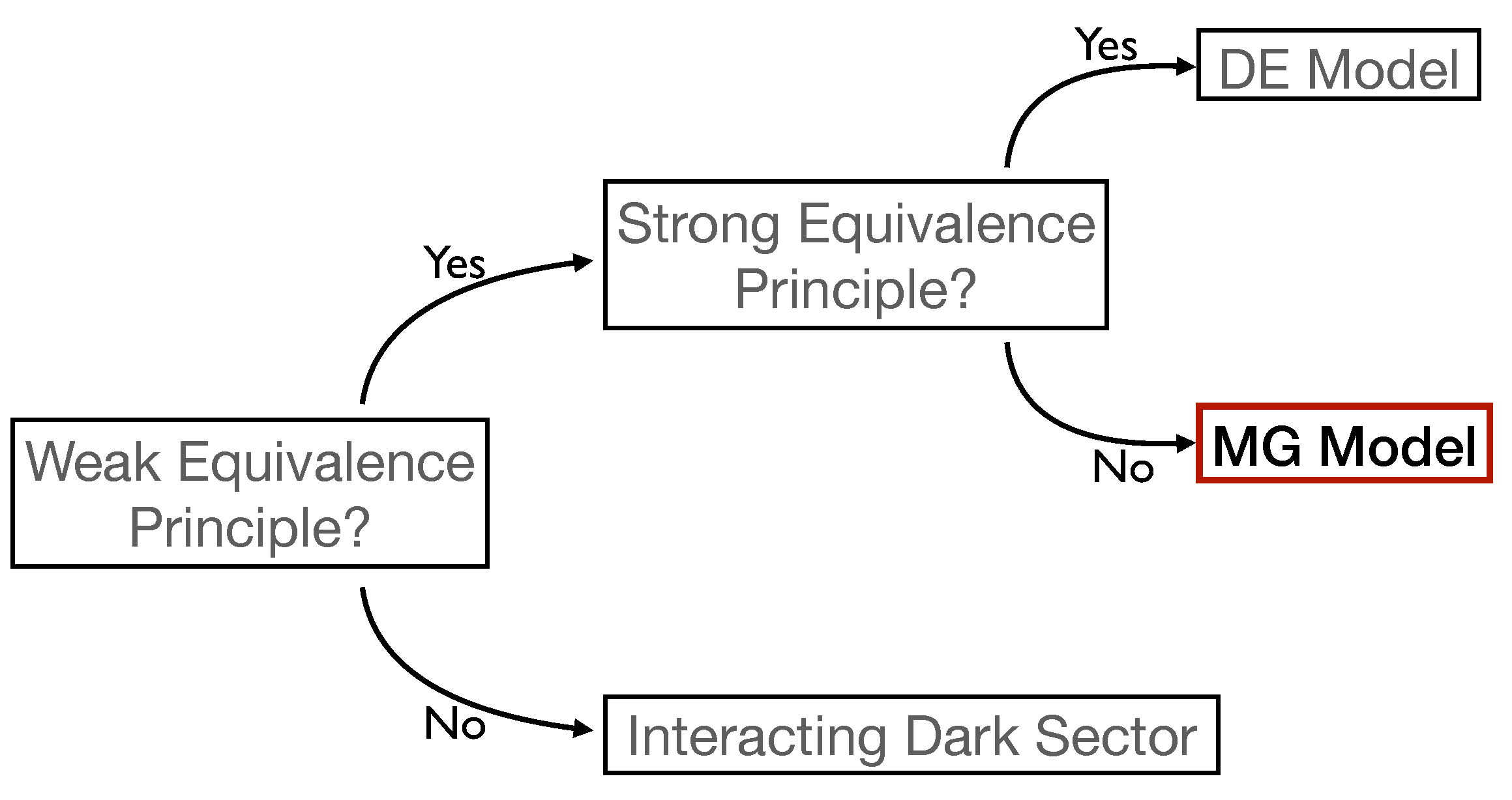
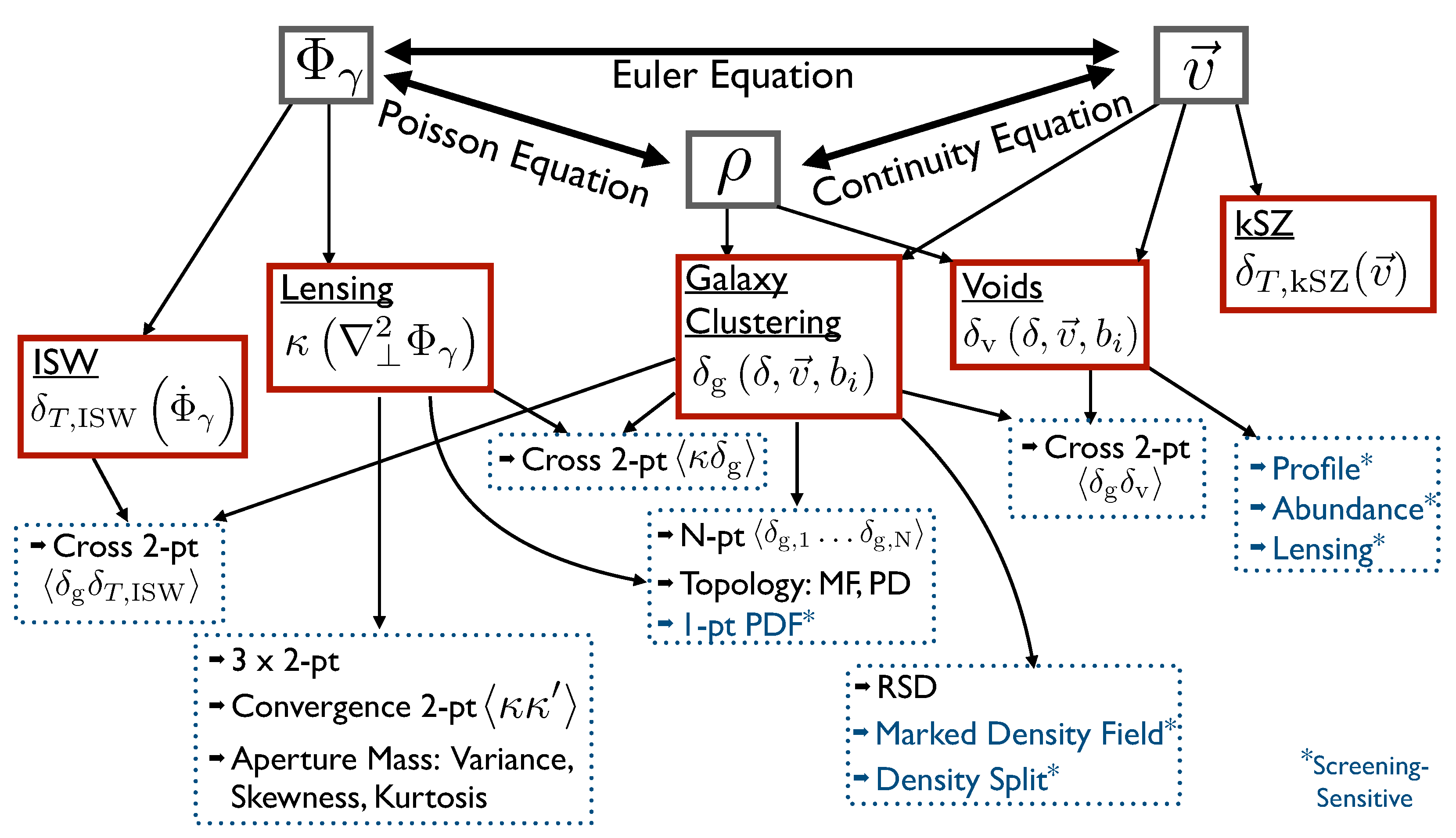
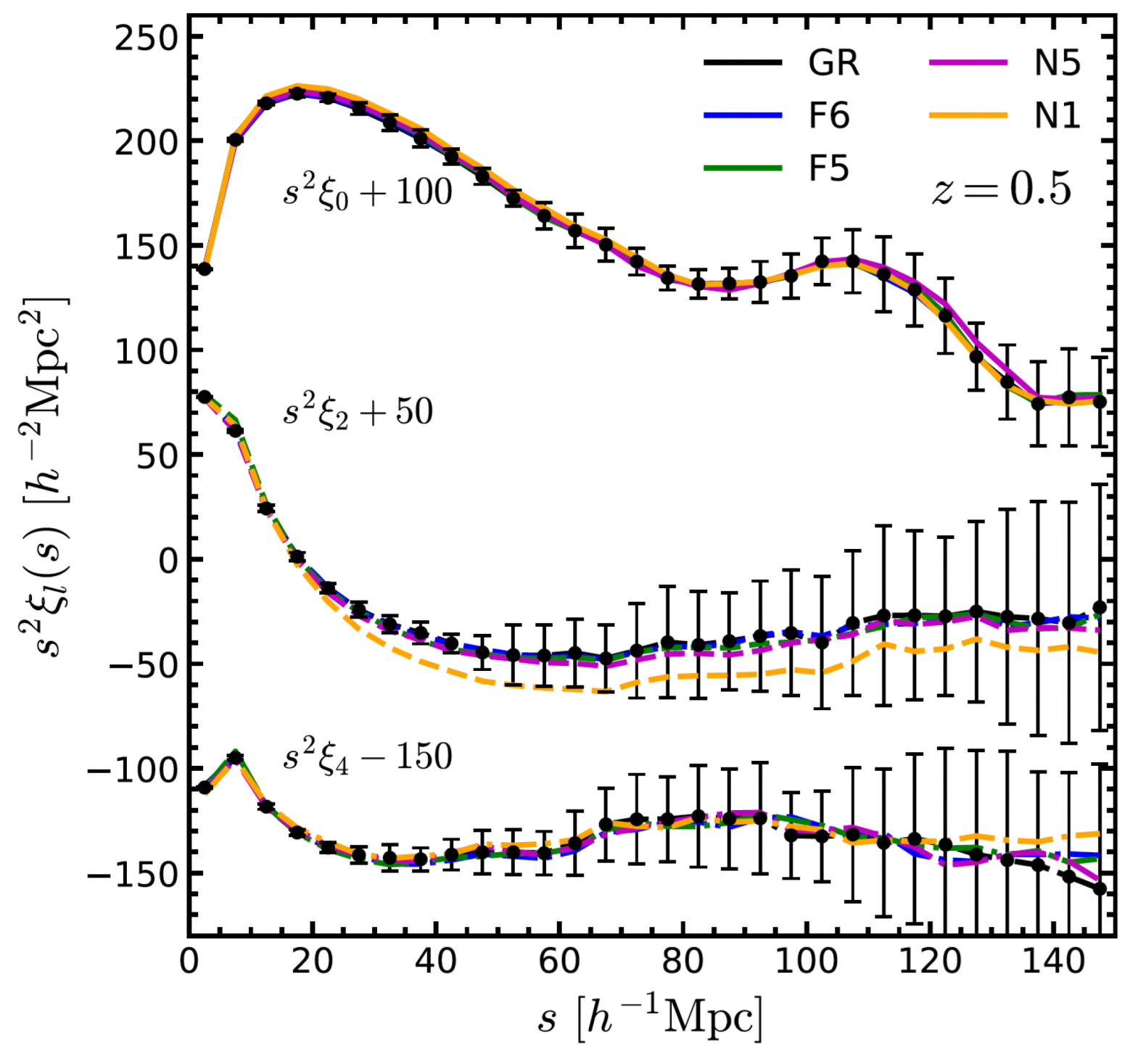
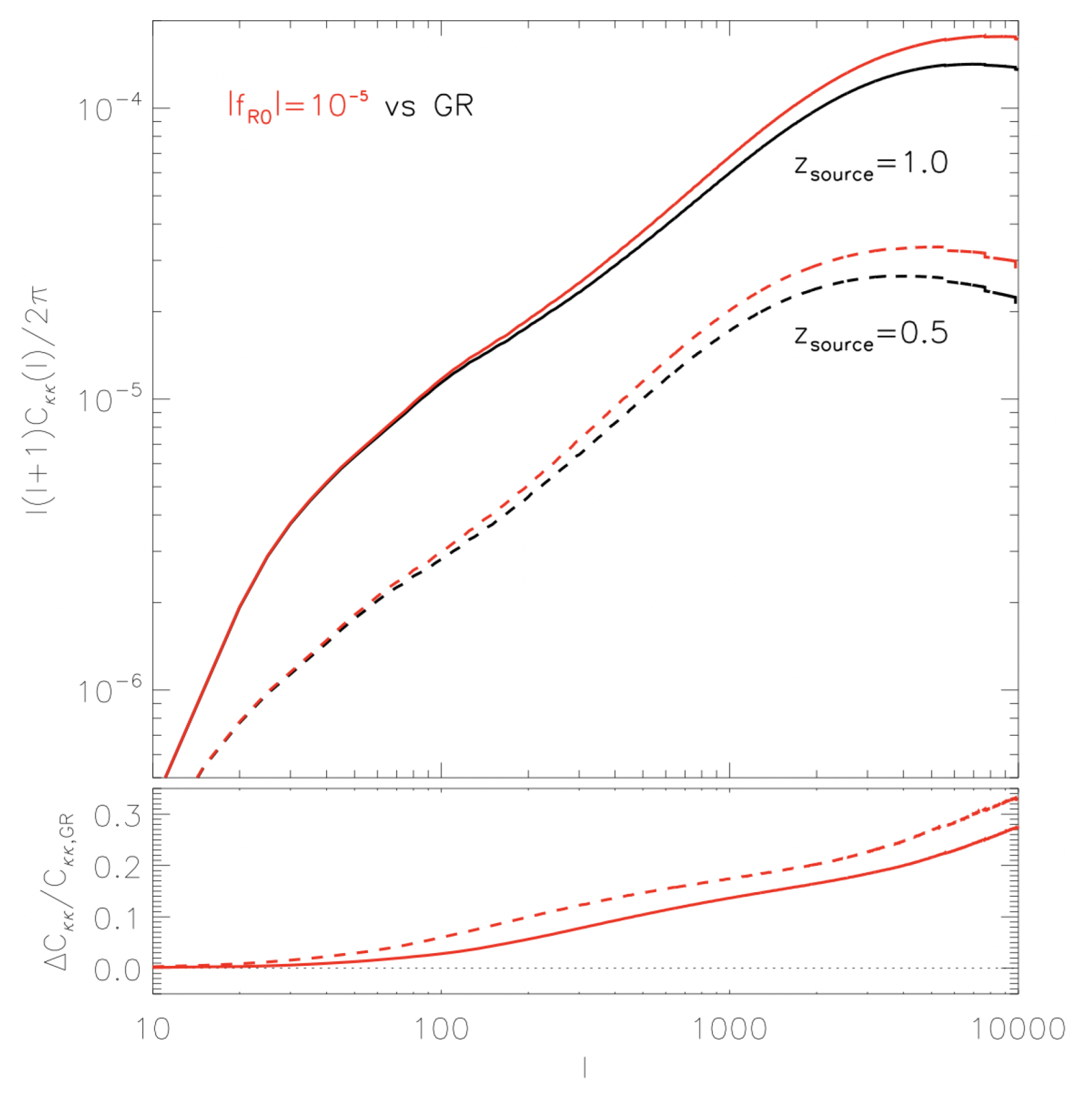
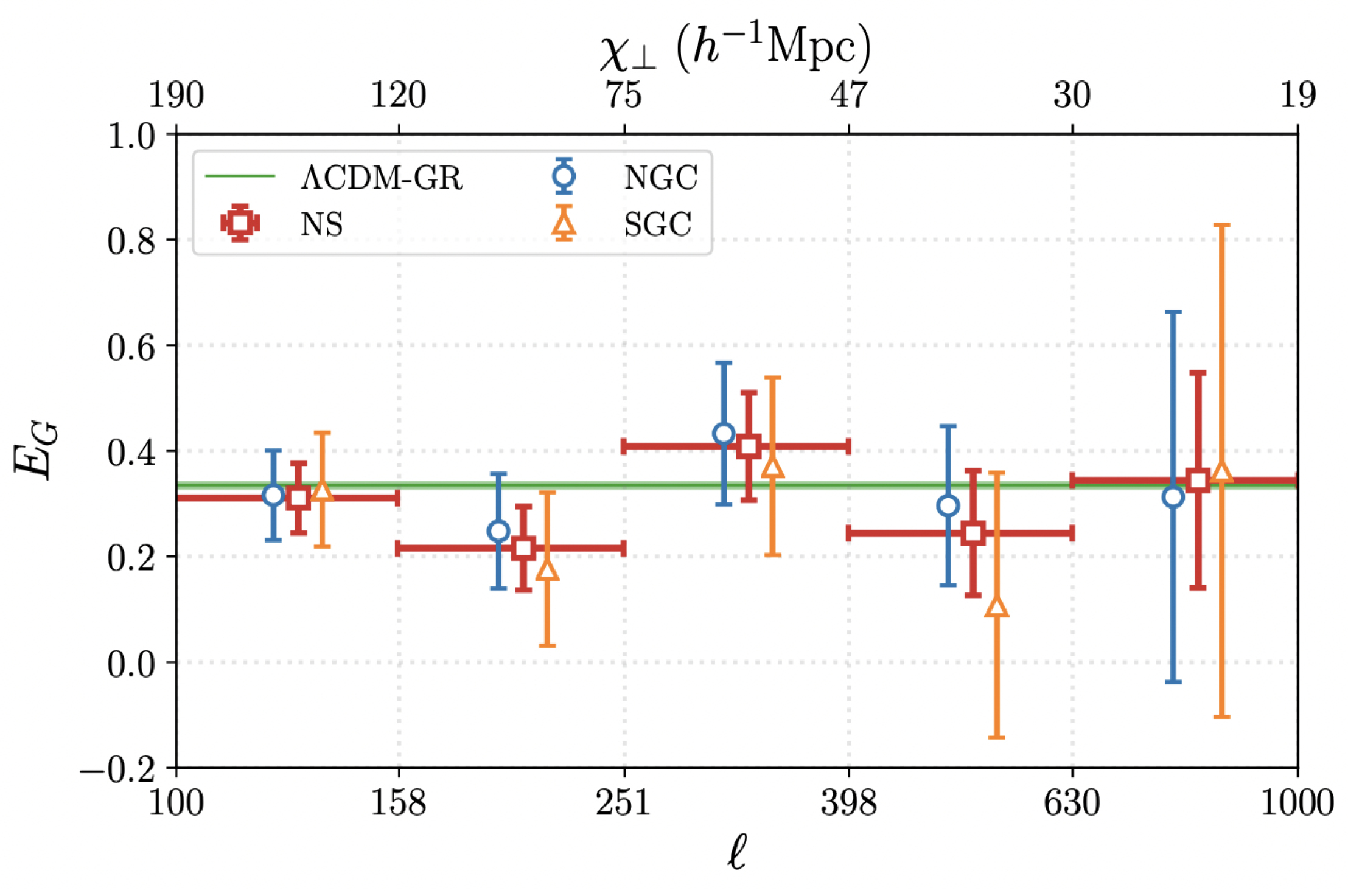
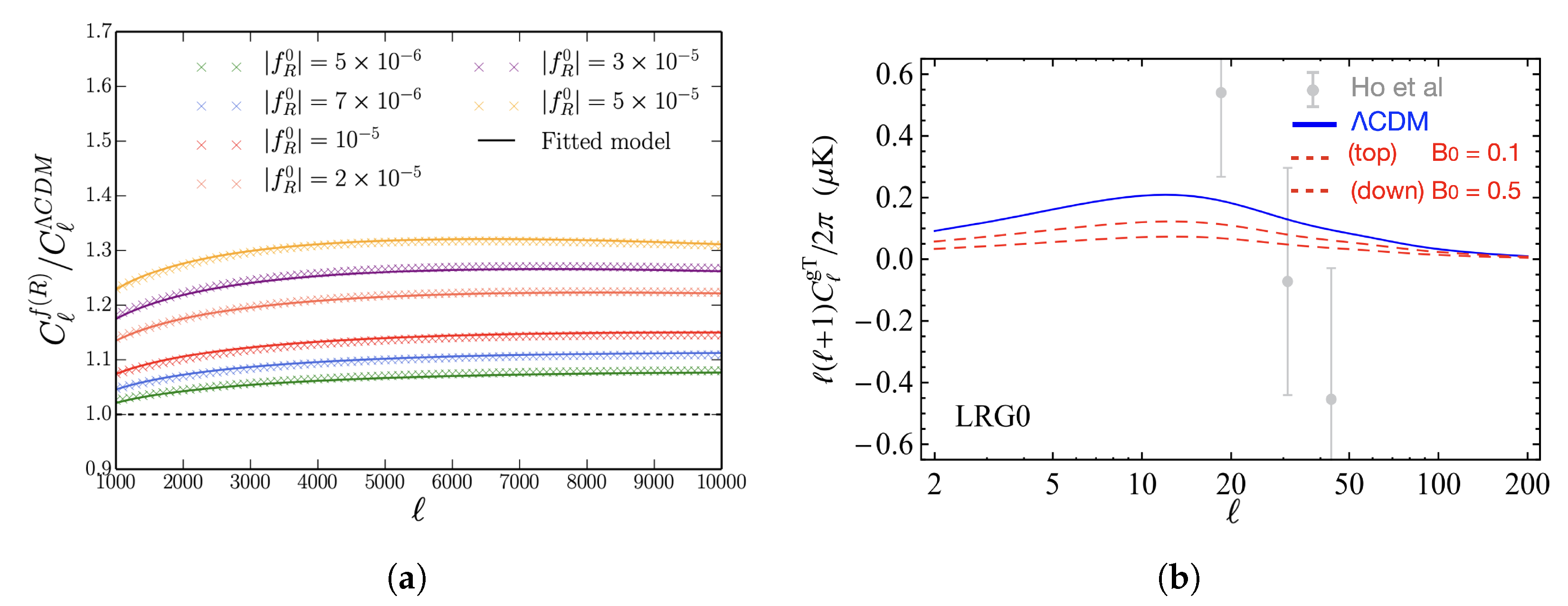
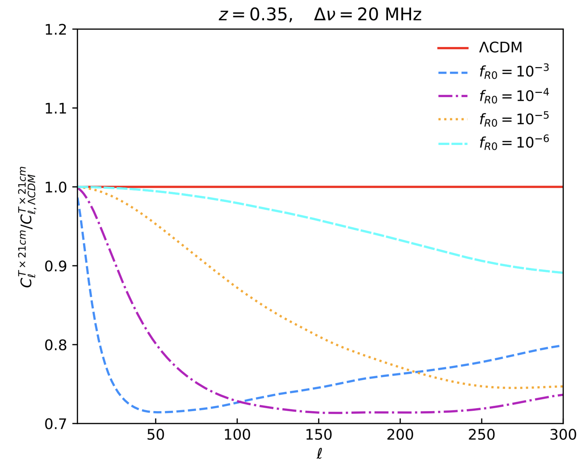
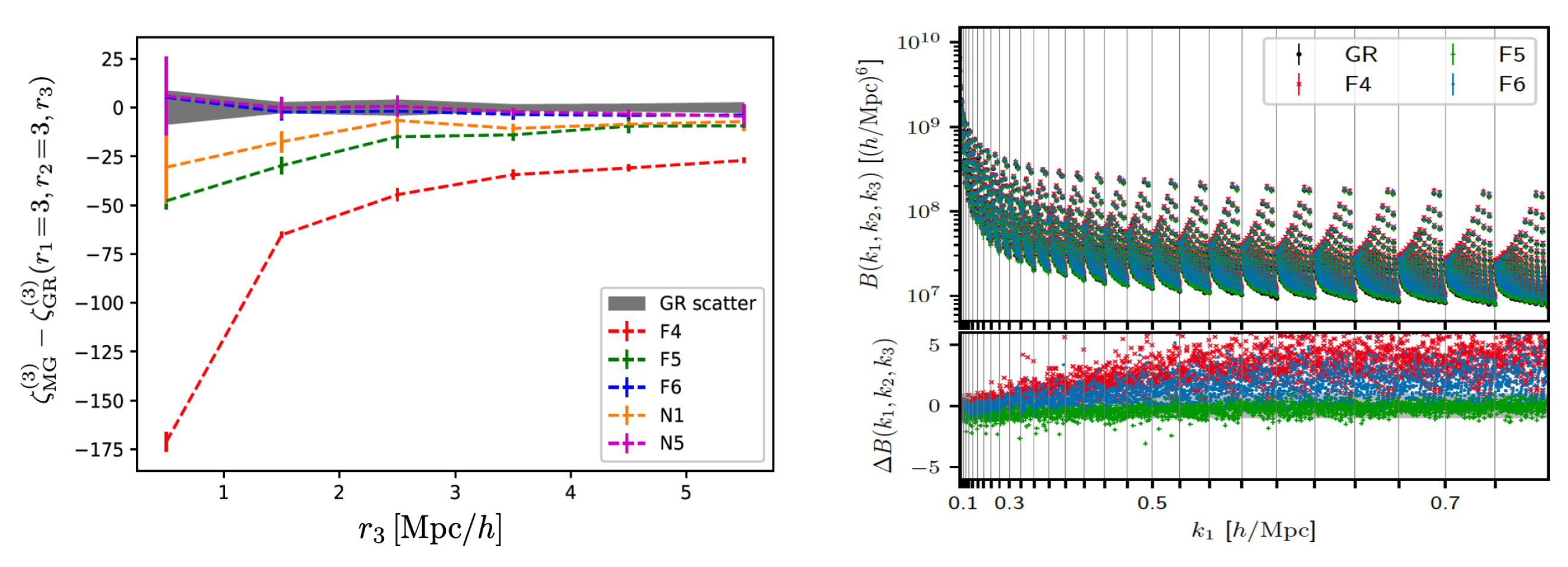
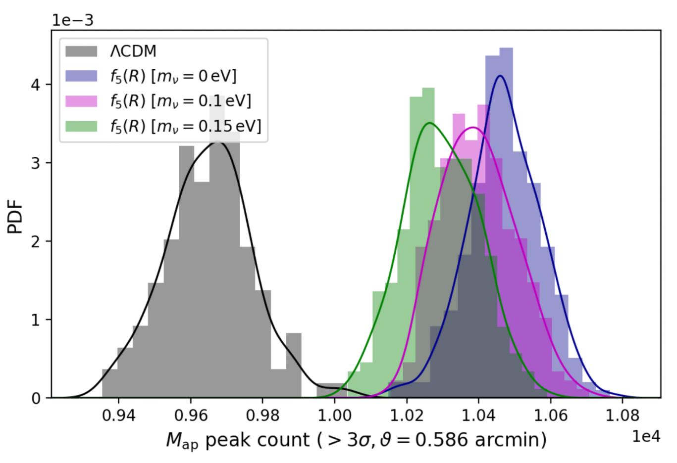
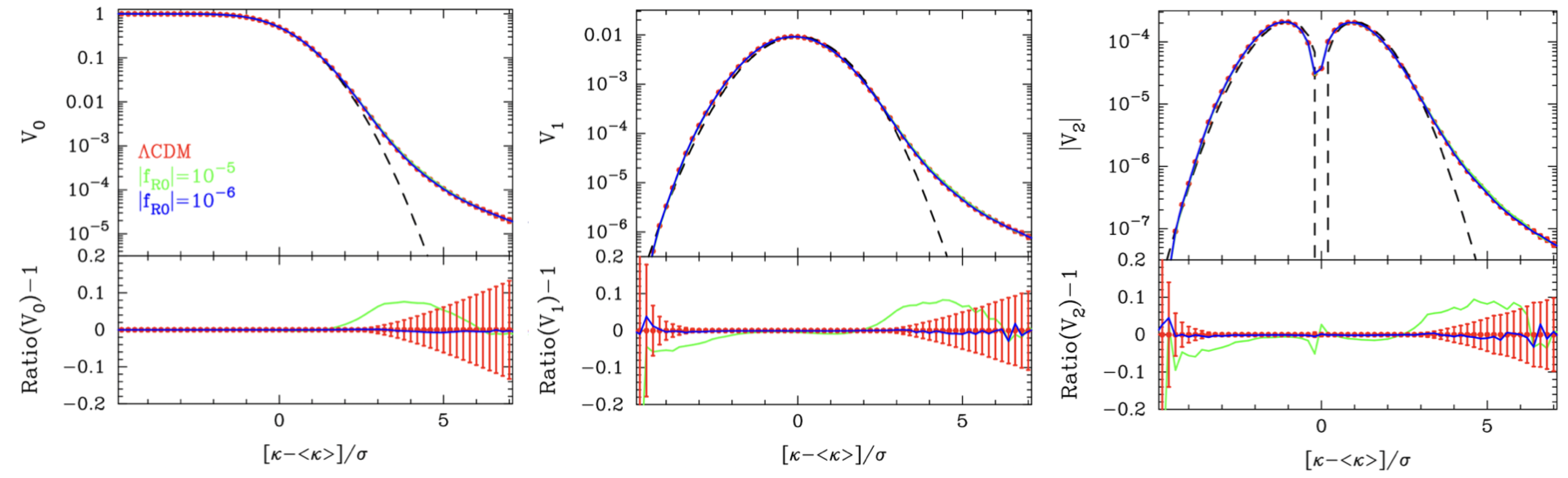
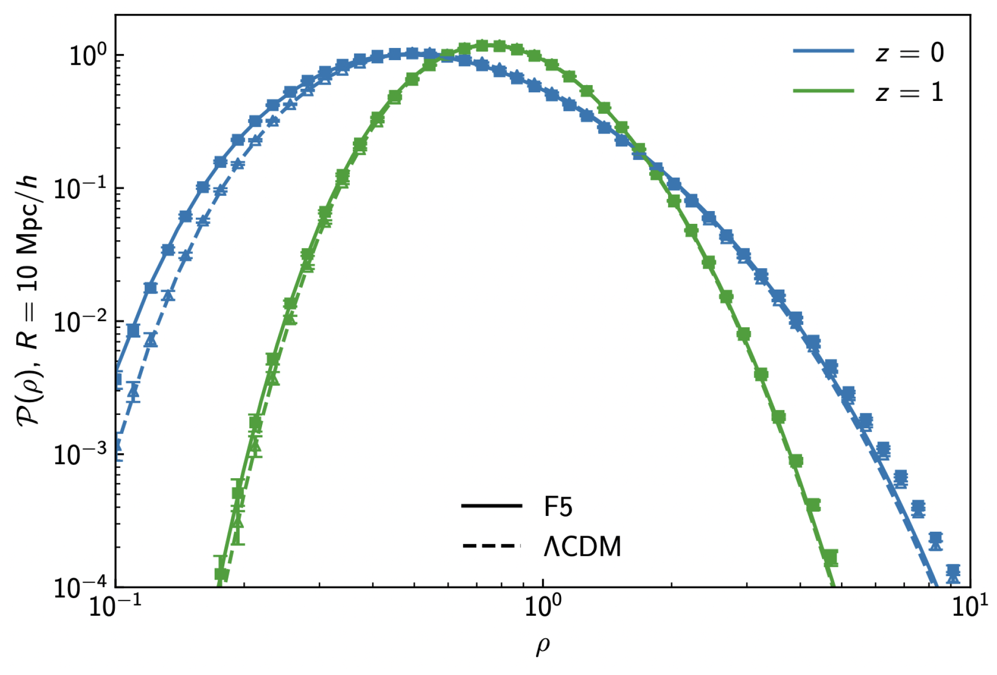
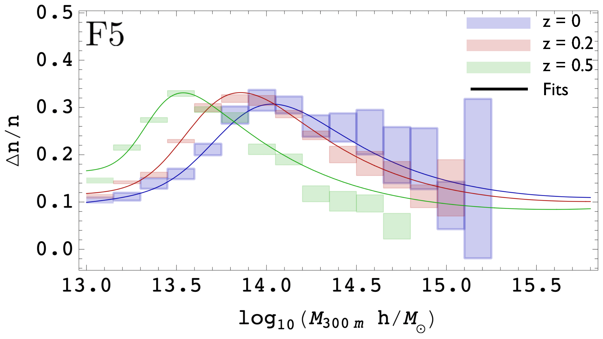
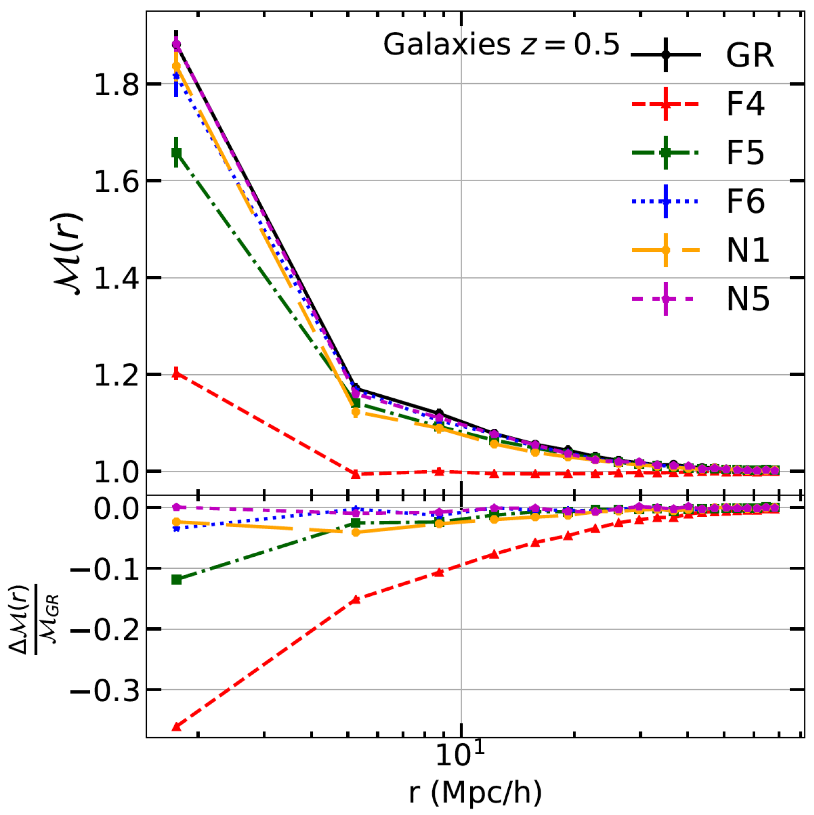
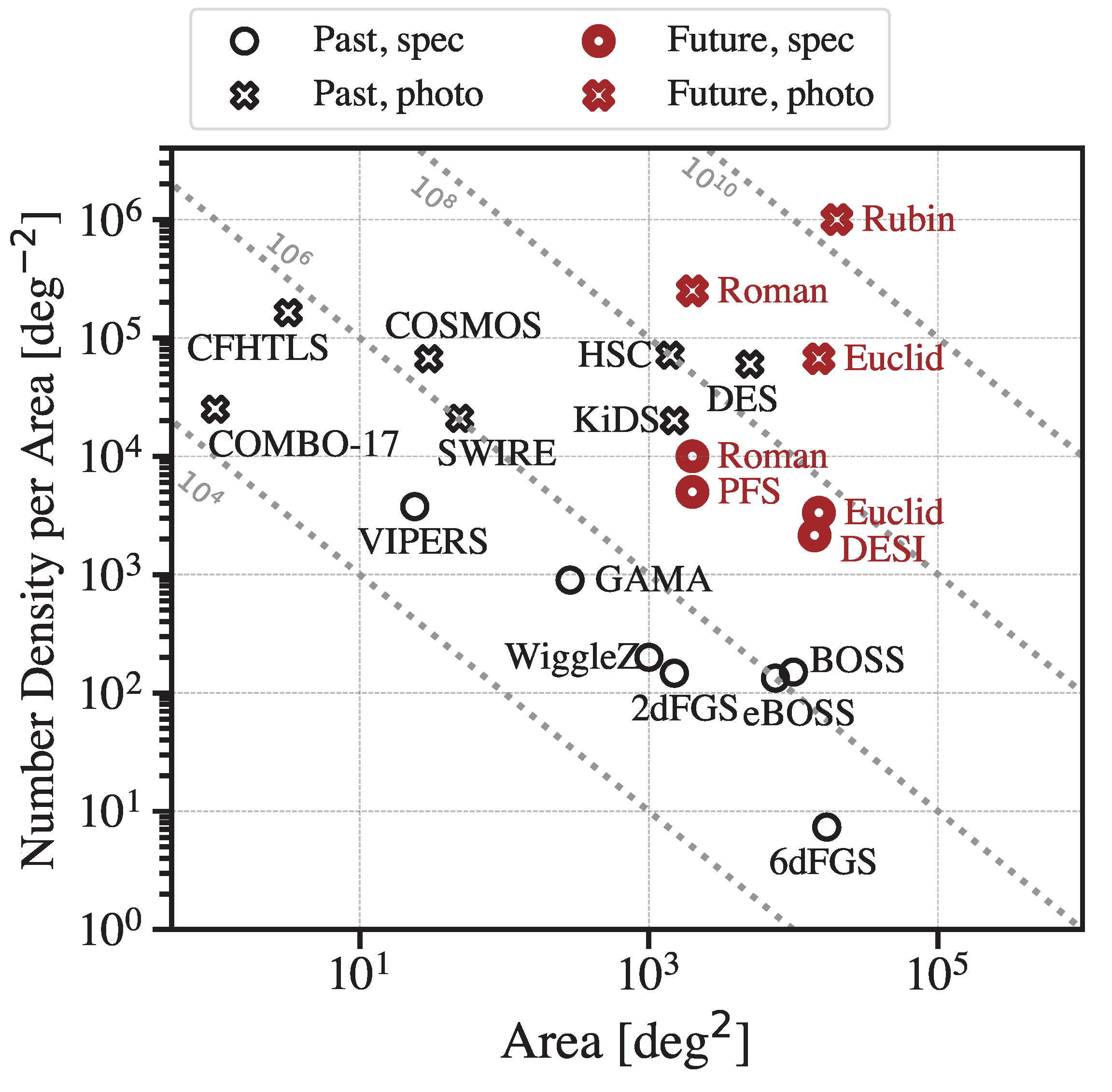
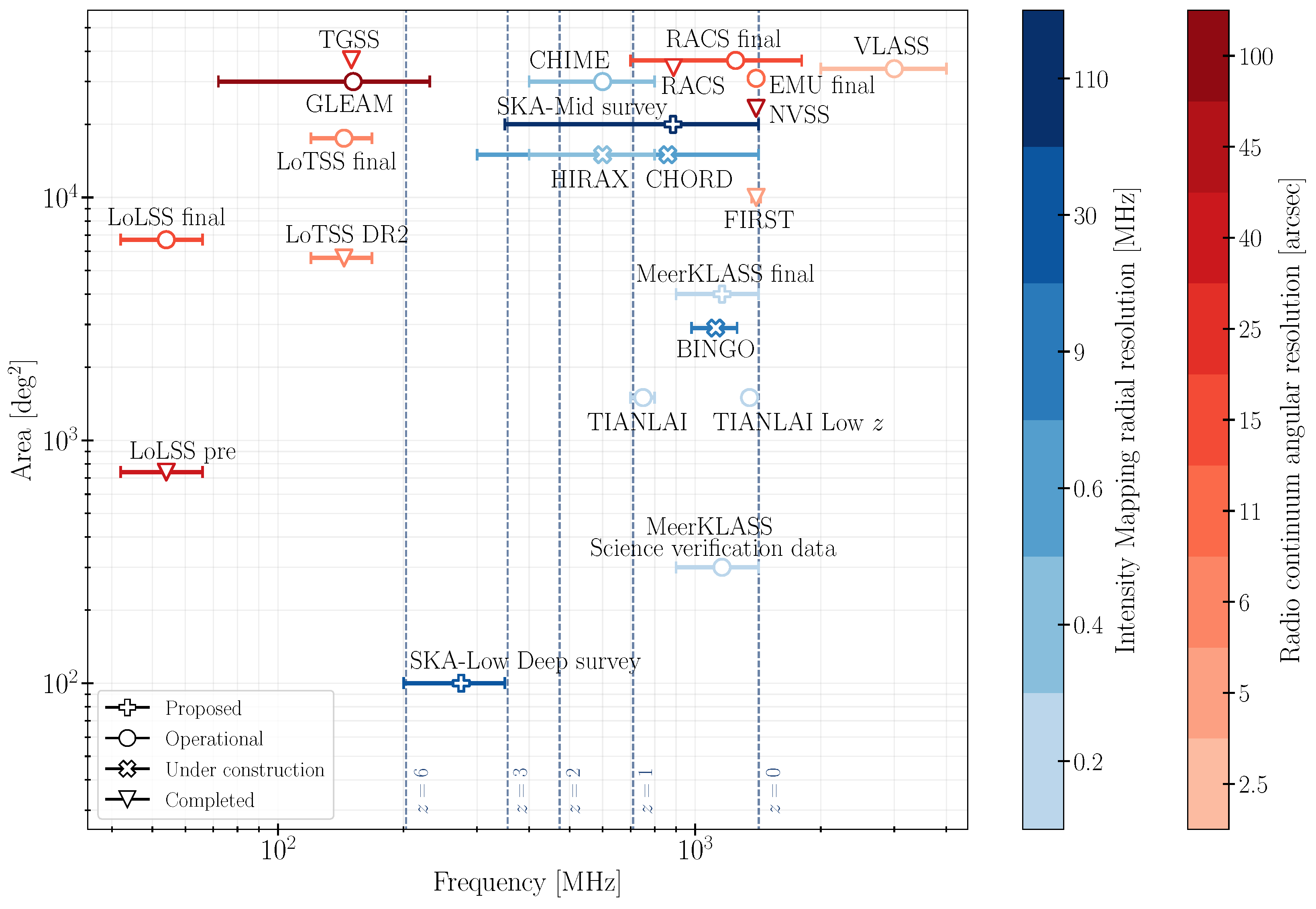
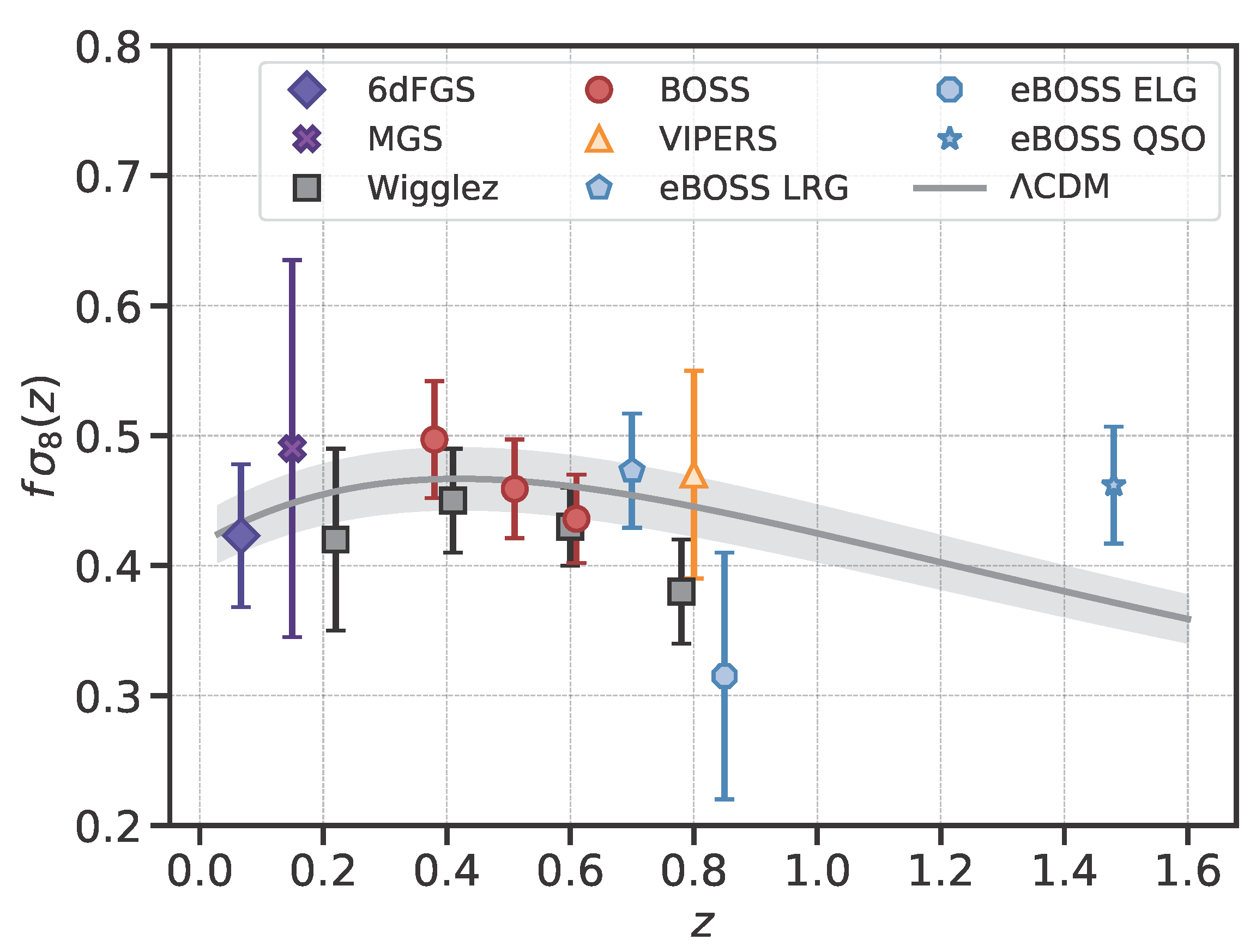
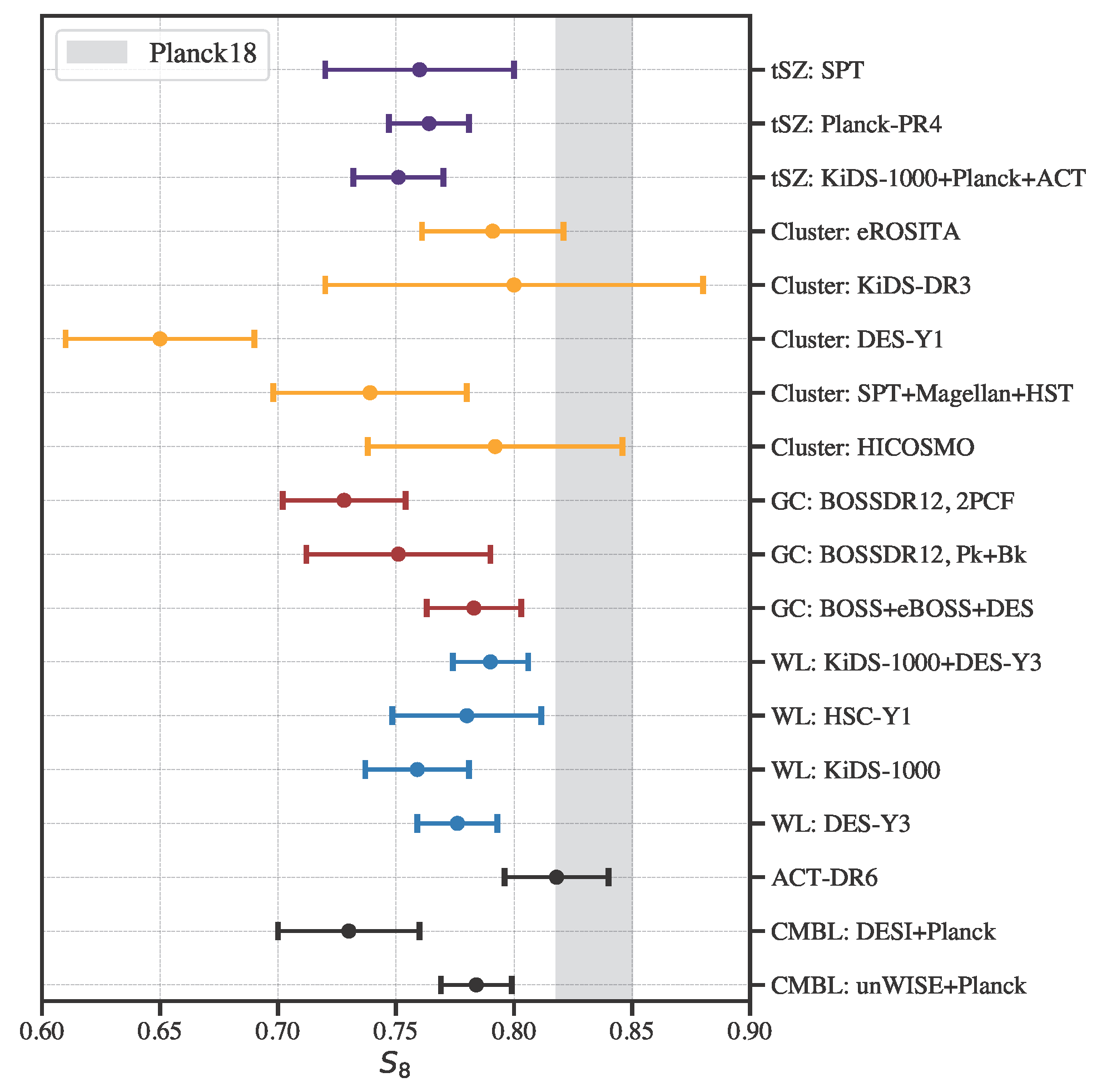
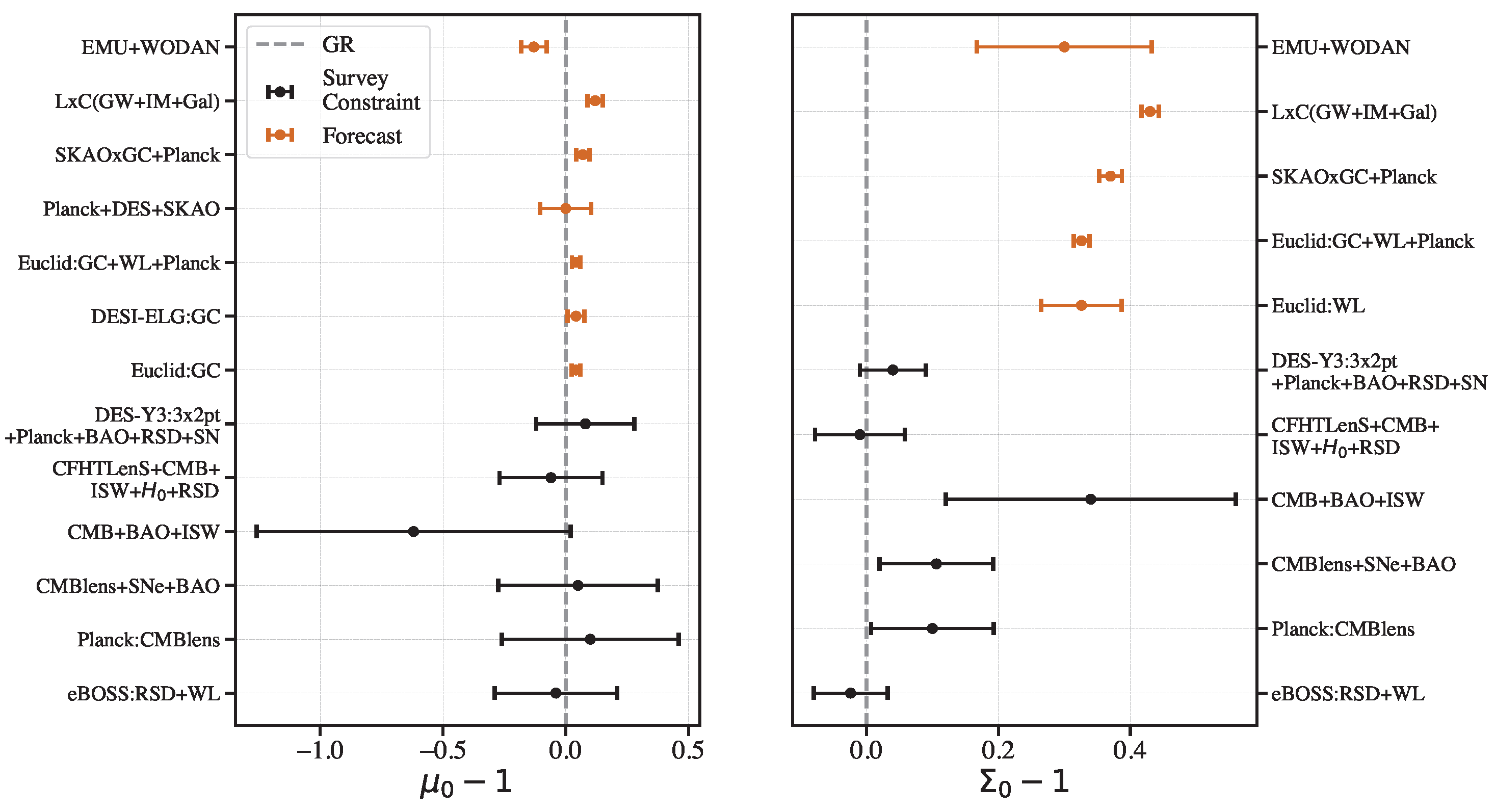
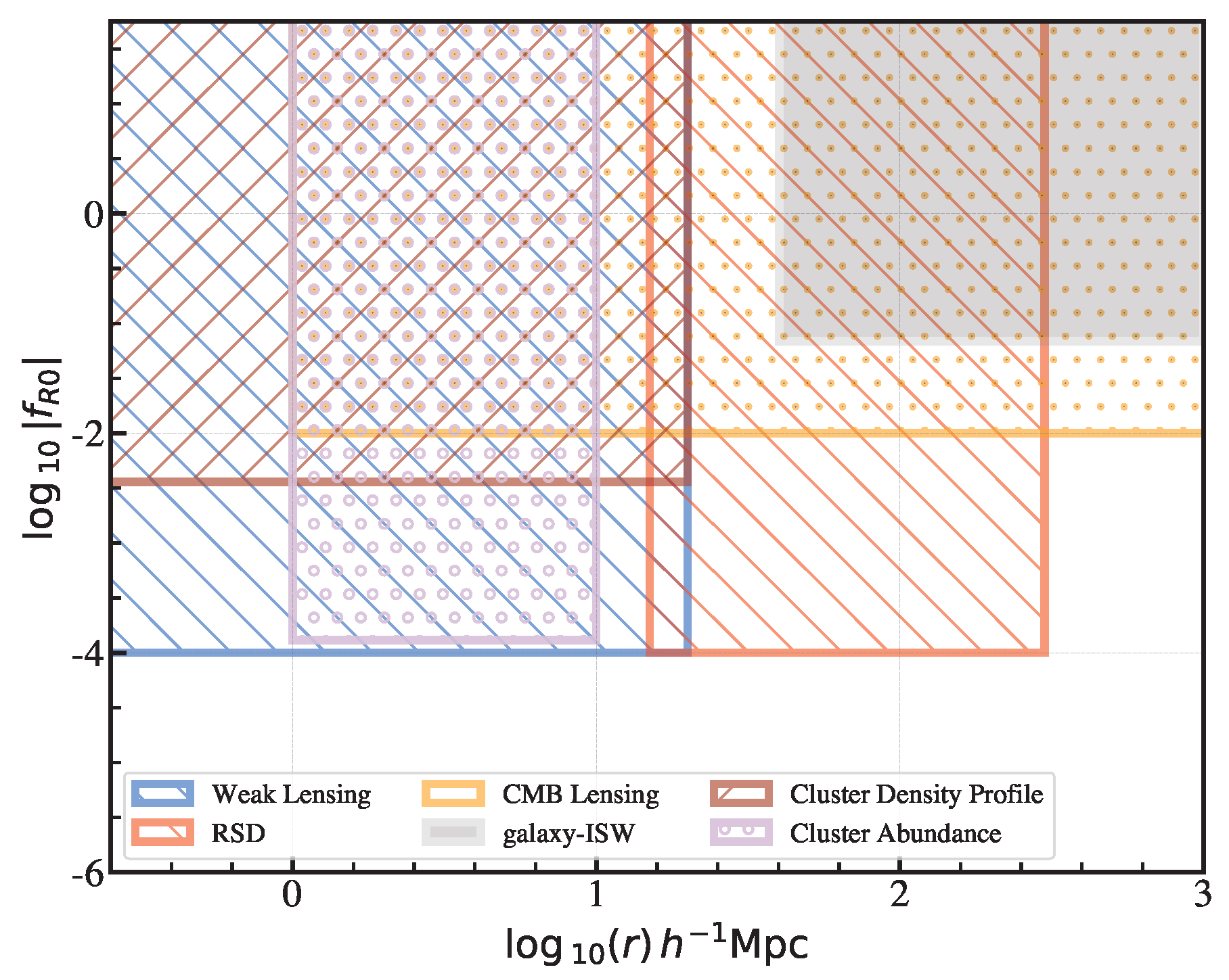
Figure 1. A flowchart distinguishing the DE and modified gravity (MG) models (based on Joyce et al. [11]). The weak equivalence principle (WEP) states that there exists a Jordan frame metric to which matter species are minimally coupled, independent of their composition or structure. Taking scalar–tensor theory as an example, all matter species couple universally to the metric in the presence of a scalar field. The strong equivalence principle (SEP) further restricts the WEP such that the equivalence principle also applies to objects that exert a self-gravitational force. If the coupling between matter fields and the metric does not involve any scalar fields, it is termed a DE model Whereas if the matter fields couple to the metric non-trivially via the scalar field, it is termed a MG model (red box) to be considered in this paper.
Universe 09 00302 g001
Figure 2. Connections between the basic physical quantities (boxed in grey) and derived observables (boxed in red). The derived observables can form different combinations as observational probes in terms of summary statistics, topological properties, and environmental dependence (boxed in dotted blue). We also highlight the probes sensitive to the screening mechanism in blue. They are useful tools in probing deviations from GR. More details see Section 3.
Universe 09 00302 g002
Figure 3. Impact of MG on the galaxy two-point correlation function multipoles at a snapshot z = 0.5 . For visibility, the multipole moments = 0 , 2 , 4 are shifted by a constant, respectively. GR is in black with error bars inferred from the standard deviation of five simulations. Coloured curves denote different MG models. A clear deviation from GR can be seen for the quadrupole moments ζ 2 , while other models are consistent within the 1 σ error bar of GR. (Credit:Hernández-Aguayo et al. [115]).
Universe 09 00302 g003
Figure 4. Upper: Convergence power spectrum (see Equation (38) with kernel Equation (40)) for GR (black) and F5 model | f ( R ) | = 10 5 at two source redshifts z source = 0.5 (dashed) and z source = 1.0 (solid). Lower: fractional difference in the convergence power spectrum for GR and F5 model (Credit: [139]).
Universe 09 00302 g004
Figure 5. E G statistic by cross-correlating the Planck CMB lensing map and eBOSS DR16 QSO sample for the Northern Galactic Cap (NGC, blue), Southern Galactic Cap (SGC, orange), and the combined sky (NS, red). The green solid line denotes the Λ CDM using Planck [182] with the shaded area being 1 σ uncertainty from the simulation. The E G probe is consistent with the scale-independent Λ CDM prediction across the five scale bins. (Credit: [179]).
Universe 09 00302 g005
Figure 7. Cross-correlation between the 21 cm and CMB temperature for different gravity models relative to the Λ CDM model. The ratio between the Λ CDM model to itself is the solid line, while the ratio of f ( R ) models are shown in dashed curves (reproduced from: [222]).
Universe 09 00302 g007
Figure 8. Impact of MG on three-point statistics. Left: difference in the 3PCF between GR (black dashed curve) and different MG models (coloured dashed curve) by fixing r 1 = r 2 = 3 h 1 Mpc only. The grey-shaded region represents the standard deviation of the five HOD GR catalogues. Right: upper panel shows the real-space bispectrum for GR (black) and the f ( R ) model (coloured). Vertical lines correspond to the k-bin interval Δ k = 0.025 Mpc 1 h . The lower panel shows the difference between GR and the MG models normalized by a combined standard deviation σ MG + GR , computed as a root-sum-squared error of the two models (reproduced from: Alam et al. [98]).
Universe 09 00302 g008
Figure 9. Peak count of aperture mass. The PDF has a clean separation for the GR and MG cases, even in the presence of massive neutrinos (reproduced from [276]).
Universe 09 00302 g009
Figure 10. Impact of f ( R ) gravity on the Minkowski functionals (MFs) of the convergence field K for V 0 (area), V 1 (total boundary length), and V 2 (integral of geodesic curvature along the contour). The x-axis is the signal-to-noise ratio of the smoothed convergence field. The MFs (coloured dots) are the average of 100 simulations with the error bars being the standard error of the mean σ std / 100 . The analytic prediction for a Gaussian random field (GRF) is shown in the black dashed curve (reproduced from [277]).
Universe 09 00302 g010
Figure 11. Global shape of the matter PDF for F5 (triangle) and Λ CDM (square) at redshift z = 0 (blue) and z = 1 (green). The measurement from the simulation is shown as the dashed curve and the model prediction is the solid curve. The f ( R ) gravity modifies the skewness of the distribution and leads to an asymmetric enhancement over Λ CDM (reproduced from Cataneo et al. [304]).
Universe 09 00302 g011
Figure 12. Relative enhancement of the halo mass function for the F5 model at z = 0 (purple), z = 0.2 (red), and z = 0.5 (green) measured from simulation (rectangles) and fits (solid curves); compared with the full simulation (blue squares) and simulations without chameleon (red triangles, displaced horizontally for visibility) (reproduced from [317]).
Universe 09 00302 g012
Figure 13. Gravitational potential marked correlation function. (Credit: Alam et al. [98]).
Universe 09 00302 g013
Figure 14. Landscape of past (black) and current/future galaxy surveys (red) for galaxy number density per area as a function of the survey area. Photometric surveys are crosses and spectroscopic surveys are open circles. The grey dotted lines corresponds to 10 4 , 10 6 , 10 8 , and 10 10 galaxies. Overall, the current/future surveys cover a larger area with a higher number density per area.
Universe 09 00302 g014
Figure 15. A summary of radio surveys. The warm red colours denote the radio continuum maps while the cold blue colours represent the 21 cm intensity mapping. The error bars show the frequency ranges for each of the instruments or surveys. While the advantage of radio surveys is their high-angular resolutions, the surveys that measure the 21 cm signal possess good high-radial resolution, i.e., the frequency and its corresponding redshifts (dashed blue vertical lines). We mark the two kinds of resolutions as different colour gradients.
Universe 09 00302 g015
Figure 16. A compiled diagram for f σ 8 ( z ) as a function of redshift from different galaxy spectroscopic surveys. The solid grey line denotes the Λ CDM with best fitting parameters from Planck15 [531] with a 5% error bar. The data points are from the following galaxy spectroscopic surveys utilizing the large-scale RSD information: 6dFGS [522], WiggleZ [523], MGS sample [524], VIPERS [525], BOSS LRG sample [521], eBOSS LRG [526,527], eBOSS ELG [528,529], and eBOSS QSO samples [181,530].
Universe 09 00302 g016
Figure 17. A compiled diagram for S 8 = σ 8 Ω m / 0.3 for CMB lensing (black) [151,171,533], galaxy WL data (blue) [133,135,136,549], galaxy clustering (red) [425,534,535], galaxy clusters (yellow) [536,537,538,539,540], and tSZ (purple) [541,542,543]. The grey band is from Planck using TT+TE+EE+lowE [182]. An intriguing 2 σ level tension in several low-redshift experiments exists when compared to the primary CMB data.
Universe 09 00302 g017
Figure 18. Constraints (black) and forecasts (orange) for μ 0 = μ | z = 0 and Σ 0 = Σ | z = 0 . From bottom to top we have RSD+WL [566], CMB lensing from Planck [182], or Planck CMB lensing+SupernovaeI+BAO [182], CMB+ISW+RSD together with a H 0 prior with or without WL data from CFHTLenS [567], and DES-Y3+Planck+BAO+RSD+SN [568]. The Euclid and DESI-ELG forecast for galaxy clustering and WL only [82], SKAO radio forecast with Planck and DES data [495], SKAO radio forecast with Planck and galaxy-clustering data [505], joint forecast using WL and clustering of GW+IM+galaxies [504], and the radio continuum surveys WODAN+EMU [192].
Universe 09 00302 g018
Figure 19. Constraints on f ( R ) from the past and current surveys. CMB lensing (SPT, ACT, Planck; [569,570,571]), galaxy power spectrum RSD (SDSS; [572]), galaxy−ISW cross−correlation (WMAP, SHOES, SCP, SDSS; [188,189,573]), cluster abundance (Chandra, MaxBCG; [189,574,575]), cluster density profile (MaxBCG; [321]), and WL (CFHTLenS; [576])19.
Universe 09 00302 g019
Table 1. Connection between well-known models of DE/MG and the EFT formalism (from Bloomfield et al. [58], Frusciante and Perenon [59]). Here, 0 means that the EFT function is identically equal to 0, ✓ indicates that the function is present, − indicates that the function is not present, while ★ indicates that the function is related to other EFT functions. In addition, we also show the relationship between different gravity models and the phenomenological functions μ , Σ , and η . For each case, it is sufficient to specify two of these functions, as the remaining functions can be derived from the other two.
Ω Λ c M 2 4 M ¯ 1 3 M ¯ 2 2 M ¯ 3 2 M ^ 2 m 2 2 μ Σ η
Λ CDM0111
f ( R ) 1 1 1
Brans–Dicke 1 1 1
Quintessence0111
k-essence0 1 1 1
DGP✓ ★ 1 1 1
Horndeski✓ ★✓ ★ ( μ 1 ) ( Σ 1 ) > 0 1 1
Disclaimer/Publisher’s Note: The statements, opinions and data contained in all publications are solely those of the individual author(s) and contributor(s) and not of MDPI and/or the editor(s). MDPI and/or the editor(s) disclaim responsibility for any injury to people or property resulting from any ideas, methods, instructions or products referred to in the content.

