

Diagnostics of Flare Loop Parameters in Shrinkage and Ascent Stages Using Radio, X-ray, and UV Emission
Abstract
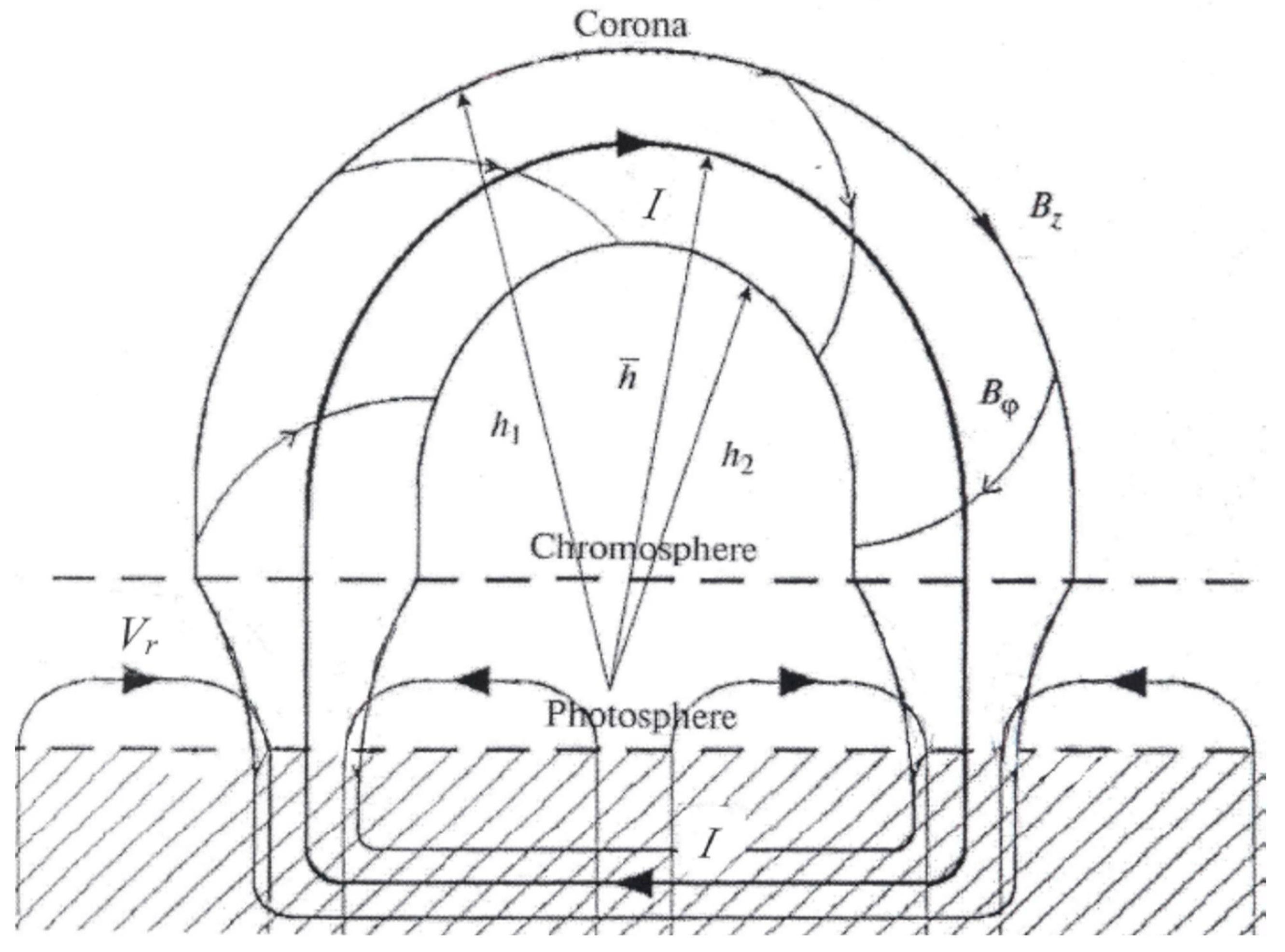
:1. Introduction
2. Loop Shrinkage in Terms of an Equivalent Electric Circuit
3. An Oscillating Loop as an Equivalent RLC Circuit
4. Dynamics of Flare Loop Parameters Inferred from Multi-Wavelength Observations
4.1. Loop in the Flare on 24 August 2002
- (i)
- In the shrinking phase (00:53–01:02 UT), an increase in the plasma temperature by more than a factor of 2.5 is observed, as well as an increase in the plasma density in the loop, approximately by a factor of three. These changes in the parameters are accompanied by a relative increase in the electric current , approximately by the factor of 1.48.
- (ii)
- At the stage of loop ascent (01:02–01:10 UT), accompanied by relatively small oscillations at 17 and 35 GHz, the plasma density inside the loop continues to increase approximately by a factor of 1.6, and the temperature decreases from 27.6 MK to 17.7 MK. Therefore, the above estimate of the magnitude of the electric current (14) reflects a certain average value at the stage of the loop expansion because the parameters that determine the period of oscillations: plasma density and the electric current magnitude, change during oscillations.
- (iii)
- The total electric current of about 1011 A contained a flare loop with r = 3.5 × 10⁶ m means a current density of j ≈ 10−2 Am−2. This value agrees with estimates of the density of the vertical electric current found using the vector magnetograms (e.g., [21,22]). In more powerful flares, the value of j can be an order of magnitude larger.
4.2. Loop in the Flare on 16 April 2002
5. Conclusions
Author Contributions
Funding
Institutional Review Board Statement
Informed Consent Statement
Data Availability Statement
Conflicts of Interest
References
- Sui, L.; Holman, G.D. Evidence for the Formation of a Large-Scale Current Sheet in a Solar Flare. Astropys. J. 2003, 596, L251–L254. [Google Scholar] [CrossRef]
- Sui, L.; Holman, G.D.; Dennis, B.R. Evidence for Magnetic Reconnection in Three Homologous Solar Flares Observed by RHESSI. Astropys. J. 2004, 612, 546–556. [Google Scholar] [CrossRef]
- Li, Y.P.; Gan, W.Q. The shrinkage of flare radio loops. Astropys. J. 2005, 629, L137–L139. [Google Scholar] [CrossRef]
- Li, Y.P.; Gan, W.Q. The oscillatory shrinkage in TRACE 195 A loops during a flare impulsive phase. Astropys. J. 2006, 644, L97–L100. [Google Scholar] [CrossRef]
- Shen, J.; Zhou, T.; Ji, H.; Wang, N.; Cao, W.; Wang, H. Early abnormal temperature structure of X-ray loop-top source of solar flares. Astrophys. J. 2008, 686, L37–L40. [Google Scholar] [CrossRef]
- Reznikova, V.E.; Melnikov, V.F.; Shibasaki, K. Dynamics of the Flaring Loop System of 2005 August 22 Observed in Microwaves and Hard X-rays. Astrophys. J. 2010, 724, 171–181. [Google Scholar] [CrossRef]
- Zhou, T.H.; Wang, J.F.; Li, D.; Song, Q.W.; Melnikov, V.; Ji, H.S. The contracting and unshearing motion of flare loops in the X7.1 flare on 2005 January 20 during its rising phase. Res. Astron. Astrophys. 2013, 13, 526–536. [Google Scholar] [CrossRef]
- Veronig, A.M.; Karlický, M.; Vršnak, B.; Temmer, M.; Magdalenić, J.; Dennis, B.R.; Ortuba, W.; Pötzi, W. X-ray sources and magnetic reconnection in the X3.9 flare of 2003 November 3. Astron. Astrophys. 2006, 446, 675–690. [Google Scholar] [CrossRef]
- Joshi, B.; Veronig, A.; Cho, K.S.; Bong, S.C.; Somov, B.V.; Moon, Y.J.; Lee, J.; Manohran, P.K.; Kim, Y.-H. Magnetic reconnection during the two-phase evolution of a solar eruptive flare. Astrophys. J. 2009, 706, 1438–1450. [Google Scholar] [CrossRef]
- Alfven, H.; Carlquist, P. Currents in the Solar Atmosphere and a Theory of Solar Flares. Solar Phys. 1967, 1, 220–228. [Google Scholar] [CrossRef]
- Zaitsev, V.V.; Stepanov, A.V.; Urpo, S.; Pohjolainen, S. LRC-circuit analog of current-carrying magnetic loop: Diagnostics of electric parameters. Astron. Astrophys. 1998, 337, 887–896. [Google Scholar]
- Zaitsev, V.V.; Stepanov, A.V. Evolution of Electric Current and Resistance in the Flare Loop in the Course of Loop Shrinkage. Geomag. Aeron. 2020, 60, 915–920. [Google Scholar] [CrossRef]
- Wang, T.J.; Solanki, S.K. Vertical oscillations of a coronal loop observed by TRACE. Astron. Astrophys. 2004, 421, L33–L36. [Google Scholar] [CrossRef]
- Hagyard, M.J. Observed nonpotential magnetic fields and the inferred flow of electric currents at a location of repeated flaring. Solar Phys. 1988, 115, 107–124. [Google Scholar] [CrossRef]
- Tan, B. Distribution of electric current in solar plasma loops. Adv. Space Sci. 2007, 39, 1826–1830. [Google Scholar] [CrossRef]
- Stepanov, A.V.; Zaitsev, V.V.; Nakariakov, V.M. Coronal Seismology: Waves and Oscillations in Stellar Coronae; Wiley-VCH Verlag GmbH&Co: Weinheim, Germany, 2012; pp. 23–29. ISBN 9783527645985. [Google Scholar] [CrossRef]
- Zaitsev, V.V.; Stepanov, A.V. Prominence activation by increase in electric current. JASTP 2018, 179, 149–153. [Google Scholar] [CrossRef]
- Klimchuk, J.A. Cross-Sectional Properties of Coronal Loops. Solar Phys. 2000, 193, 53–75. [Google Scholar] [CrossRef]
- Zaitsev, V.V.; Kronshtadtov, P.V. On the Constancy of the Width of Coronal Magnetic Loops. Geomag. Aeron. 2017, 57, 841–843. [Google Scholar] [CrossRef]
- Thomas, R.J.; Starr, R.; Crannell, C.J. Expressions to Determine Temperatures and Emission Measures for Solar X-Ray Events from Goes Measurements. Solar Phys. 1985, 95, 323–329. [Google Scholar] [CrossRef]
- Pevtsov, A.A.; Canfield, R.C.; McClymont, A.L. On the Subphotospheric Origin of Coronal Electric Currents. Astrophys. J. 1997, 491, 973–977. [Google Scholar] [CrossRef]
- Sharykin, I.N.; Kosovichev, A.G. Dynamics of Electric Currents, Magnetic Field Topology, and Helioseismic Response of a Solar Flare. Astrophys. J. 2015, 808, 72–81. [Google Scholar] [CrossRef]
- Aschwanden, M.J.; Newmark, J.S.; Delaboudinière, J.P.; Neupert, W.M.; Klimchuk, J.A.; Gary, G.A.; Portier-Fozzani, F.; Zucker, A. Three-dimensional Stereoscopic Analysis of Solar Active Region Loops. I. SOHO/EIT Observations at Temperatures of (1.0–1.5) × 106 K. Astrophys. J. 1999, 515, 842–867. [Google Scholar] [CrossRef]
- Giampapa, M.S.; Rosner, R.; Kashyap, V.; Fleming, T.A.; Schmitt, J.H.M.M.; Bookbinder, J.A. The Coronae of Low-Mass Dwarf Stars. Astrophys. J. 1996, 463, 707–725. [Google Scholar] [CrossRef]


| Flare Phase | /109 cm | R/10−2 | EM/1049 cm−3 | V/1027 cm3 | T MK | n/1010 cm−3 | I/1010 A |
|---|---|---|---|---|---|---|---|
| Flare start 00:49 UT | 2.3 | 7.0 | 0.38 | 2.80 | 9.4 | 3.70 | - |
| Shrink start 00:53 UT | 2.3 | 13.3 | 0.78 | 2.80 | 11.0 | 5.28 | 8.6 |
| Shrink end 01:02 UT | 1.6 | 50.0 | 5.2 | 1.93 | 27.6 | 16.4 | 12.7 |
| Oscillations 01:00–01:10 UT | 2.45 | 31.7 | 22.0 | 2.96 | 17.7 | 27.0 | 15.9 |
Disclaimer/Publisher’s Note: The statements, opinions and data contained in all publications are solely those of the individual author(s) and contributor(s) and not of MDPI and/or the editor(s). MDPI and/or the editor(s) disclaim responsibility for any injury to people or property resulting from any ideas, methods, instructions or products referred to in the content. |
© 2023 by the authors. Licensee MDPI, Basel, Switzerland. This article is an open access article distributed under the terms and conditions of the Creative Commons Attribution (CC BY) license (https://creativecommons.org/licenses/by/4.0/).
Share and Cite
Zaitsev, V.; Stepanov, A. Diagnostics of Flare Loop Parameters in Shrinkage and Ascent Stages Using Radio, X-ray, and UV Emission. Universe 2023, 9, 261. https://doi.org/10.3390/universe9060261
Zaitsev V, Stepanov A. Diagnostics of Flare Loop Parameters in Shrinkage and Ascent Stages Using Radio, X-ray, and UV Emission. Universe. 2023; 9(6):261. https://doi.org/10.3390/universe9060261
Chicago/Turabian StyleZaitsev, Valery, and Alexander Stepanov. 2023. "Diagnostics of Flare Loop Parameters in Shrinkage and Ascent Stages Using Radio, X-ray, and UV Emission" Universe 9, no. 6: 261. https://doi.org/10.3390/universe9060261