

Do White Holes Exist?


1
Institute of Space Sciences (ICE, CSIC), 08193 Barcelona, Spain
2
Institut d Estudis Espacials de Catalunya (IEEC), 08034 Barcelona, Spain
3
Institute of Cosmology & Gravitation, University of Portsmouth, Dennis Sciama Building, Burnaby Road, Portsmouth PO1 3FX, UK
Universe 2023, 9(4), 194; https://doi.org/10.3390/universe9040194
Submission received: 9 March 2023
/
Revised: 9 April 2023
/
Accepted: 17 April 2023
/
Published: 19 April 2023
(This article belongs to the Special Issue Universe: Feature Papers 2023—Cosmology)
Abstract
:In a paper published in 1939, Albert Einstein argued that Black Holes (BHs) did not exist “in the real world”. However, recent astronomical observations indicate otherwise. Does this mean that we should also expect White Holes (WHs) to exist in the real world? In classical General Relativity (GR), a WH refers to the time reversed version of a collapsing BH solution that allows the crossing of the BH event horizon inside out. Such solution has been disputed as not possible because escaping an event horizon violates causality. Despite such objections, the Big Bang model is often understood as a WH (the reverse of a BH collapse). Does this mean that the Big Bang breaks causality? Recent measurements of cosmic acceleration indicate that our Big Bang solution is not really a WH, but a BH. Events decelerate when the expansion accelerates and this prevents the crossing of the event horizon from inside out. We present a general explanation of why this happens; the explanation resolves the above causality puzzle and indicates that such apparent WH solutions have a regular Schwarzschild BH exterior.
1. Introduction
Decades after Einstein [1] concluded that BHs did not exist, observations have shown that they are real astronomical objects [2,3,4]. A Schwarzschild Black Hole (BH) solution:
represents a singular point source of mass M. The gravitational radius corresponds to an event horizon and prevents us from seeing inside . The Schwarszchild solution applies to the exterior of any BH, no matter what the interior solution is, as long as we can approximate the outer region as empty space. The Hawking–Penrose’s theorems [5,6] tell us that nothing can come out of . This has created the BH information lost paradox [7,8]. One possible way around this is to introduce the concept of maximally extended Schwarszchild solution using the Kruskal–Szekeres coordinates and (see Figure 1), where the future BH event horizon becomes the past White Hole (WH) horizon. Information can escape in a WH. There are two disconnected exterior spaces which could be connected inside with an Einstein–Rosen bridge or Schwarszchild wormhole [9].
If we throw a particle into a BH, the WH solution corresponds to the traveling of that particle back in time to us (from our past), before the particle was sent. Such trajectory might be formally possible (because there is no arrow of time at the fundamental level), but it violates causality, so it makes no physical sense as a classical solution (quantum mechanics effects might provide some way around this [10]). This is related to the example of retarded and advanced potentials in classical electrodynamics: both are mathematical solutions of the wave equations, but only one of them connects cause and effect. The mirror image of the top quadrant in Figure 1 has the arrow pointing downward and not upward. This shows that the time reversed solution (the mirror image) is still a BH (where the particle falls into the gravitational radius ) and not a WH (as indicated in the figure).
Here we will study the more realistic case of classical Lemaitre–Tolman–Bondi (LTB) solutions, which include the FLRW metric, the Oppenheimer–Snyder BH [11] and the thin shell BH [12] as particular cases. For some reason, i.e., the difficulty of a black-to-white hole bounce (see [13,14]), these solutions are usually investigated only as BH collapsing solutions. As we will show, the same solutions also exist, in principle, as WH solutions. The most famous of this is the expanding Big Bang model originally proposed by Friedman in 1922 [15] and Lemaitre in 1927 [16]. However, at closer inspection, these solutions need to be modified to include a surface term. After that correction, we show that the WH correspond, in fact, to BH expanding solutions. Our argument is supported by considering surface terms in the Einstein–Hilbert action of classical GR and also by the recent observation that our cosmic expansion is accelerating.
2. LTB Solutions
The most general metric with spherical symmetry in spherical coordinates can be written as [17]:
Other common notation is: , and [11,18,19]. An alternative to this uses proper time :
where the radial coordinate can be comoving or not (because its evolution can be encoded in the and r functions). This last metric is sometimes called the Lemaitre–Tolman metric [16,18] or the Lemaitre–Tolman–Bondi or LTB metric. A metric such as this one, expressed with and is called synchronous (or in a synchronous frame) because time lines are geodesics. Either way, it is possible to express the spherical symmetric metric with two functions. The best form in each case depends on the energy content and the observer’s frame. In all cases, this is a local metric around a reference central point in space which we have set to be the origin ().
The advantage of using the proper time and an observer moving with a perfect fluid is that the stress tensor becomes diagonal: , where is the energy density and is the pressure. We will focus here in the matter-dominated case for simplicity, but we expect similar results to apply to more general situations (see [20]). The solution to the field equation is , where dots and primes correspond to time and radial partial derivatives. This equation can be solved as , where is an arbitrary function of . The choice corresponds to the particular flat geometry case:
The solution for r in this case is easily found:
The above expression reproduces the Newtonian energy conservation in free fall: [21] and corresponds to an expanding or collapsing relativistic spherical ball. When is uniform, we find so that Equation (4) reproduces the flat FLRW metric:
and Equation (5) reproduces the corresponding solution . The next simplest solution to Equation (5) is that of the FLRW uniform cloud with a fixed total mass :
The solution is as in the standard FLRW metric but with a boundary at above which () we have empty space: .
This is a consequence of Birkhoff’s theorem [22] (or Gauss’ law in non relativistic mechanics), since a sphere cut out of an infinite uniform distribution conserves the same spherical symmetry and the solutions are independent of what is outside. If the outer region is empty space, we just recover the static Schwarzschild solution outside and the FLRW metric inside. Thus, the FLRW metric is both a solution to a global homogeneous (i.e., ) uniform background and also to the inside of a local (finite ) uniform sphere centered around one particular point. The local solution is called the FLRW cloud (FLRW*) [20]. As we will show next, the LTB solution could in principle be viewed as a BH or a WH, depending on whether the FLRW metric is expanding or collapsing.
A timelike radial geodesic () in the FLRW cloud has a mass-energy M inside which is independent of . Such fixed comoving coordinate corresponds to a system with a fixed mass inside (see also [23]), which expands or collapses following the Hubble–Lemaitre law of Equation (5).
From Equation (5), we have , where is just the value at some arbitrary time (), when R intersects , so that . This solution is time reversible and the evolution can cross in both directions. This is a well known solution which includes the Oppenheimer–Snyder BH collapse [11] and the thin shell BH [12]. However, note that when , we have (or ), which creates a region between which is acausal during expansion (this is the well known horizon problem in the standard Big Bang cosmology). We can also reproduce the same LTB (or FLRW*) solution using junction conditions to verify that the exterior of is indeed a classical (Schwarszchild) BH despite the looks of Equation (4). The original derivation [20] is reproduced here in Appendix A (with some typos corrected) for reference.
To show that this solution actually crosses the gravitational radius , we can estimate the event horizon (EH), , of the FLRW* metric. This is the maximum distance that a photon emitted at time can travel following an outgoing radial null geodesic [24]:
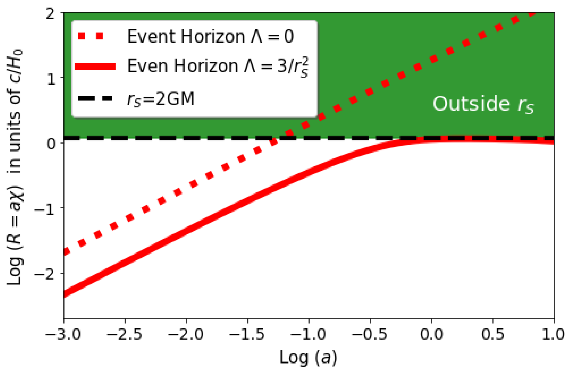
For , we have , which grows unbounded with a and therefore crosses , as shown by the dashed red line in Figure 2.
The case corresponds to a collapsing solution, and therefore, a BH. This collapsing solution is protected by the Equivalence principle, as a free fall test particle at is equivalent to a particle moving in empty space and can therefore cross . The case is expanding and is what we have labeled as a WH solution. It just corresponds to a fluid expanding inside . However, what is strange about this solution is that information can actually escape from the interior to the exterior of , which is contrary to all that we have learned about BHs and causality. How is that possible?
The standard objection to this paradox is that this expanding configuration can never be achieved. This is reflected in the fact that is not causally connected to its past (the so called horizon problem), which is a similar objection to the one for WH interpretation of the Schwarzschild solution, as discussed in the introduction. Note that this expanding solution corresponds to the matter-dominated Big Bang solution, which is very close to current observations 1. This is why it is often said that the Big Bang is a WH 2.
Here, we argue that this expanding WH solution is not correct. This is not because it cannot be achieved (as illustrated by the existence of our own observed universe). But because the gravitational radius should be interpreted as a boundary that separates the interior from the exterior manifold. This is strictly the case if the exterior is empty space (as we have assumed here) 3. Such boundary requires that we change the GR field equations. Appendix B reproduces the original calculation in [20,25] that shows that the Gibbons–Hawking–York (GHY) boundary in the action corresponds to an effective term: . We will show next how this boundary term transforms the WH solution into a BH solution.
How a WH Turns into a BH
Let us next consider how the derivation presented in Appendix A, which assumed , changes when including an effective term: inside (as suggested by the GHY boundary argument given above). Such term does not change the form of the FLRW metric itself, but (as it is well known) it changes the field equations and therefore the solution to expansion rate . But the term does change the form of the Schwarszchild solution and metric inside. The solution now is the deSitter–-Schwarzschild metric: . Thus, to find the new junction, we just need to replace F in the definition of in Equation (A4). The new second junction condition then becomes:
which is exactly the new Hubble law with and a constant mass in Equation (6). This shows that the LTB (or FLRW*) expanding metric is also a solution to the new field equations with the boundary. However, this solution is no longer a WH, but has become a BH. We can check this by estimating the new EH in Equation (9), now including the effective term in H. The new estimation for is displayed as a red continuous line in Figure 2. As can be seen, the EH is trapped inside , which indicates that no information can escape. The WH solution has now turn into a BH.
3. Conclusions
We have shown that classical WH solutions in GR can be turned into an expanding BH solutions once we account for the fact that the gravitational radius corresponds to a boundary condition in the action of GR.
The matter-dominated case study here is a very good approximation for our universe, because in the later stages of its evolution, it is totally dominated by mater and the effective . This could also be in general a good approximation for stellar or supermassive BHs with uniform density and pressure because as inside, matter and always dominate. The characteristic gravitational time is quite short:
so, even for a super massive BH (), time is measured in seconds or hours. In astronomical time-scales, the evolution is quickly dominated by the effective term inside. This, by the way, explains the coincidence problem in our Universe [26].
If we think of experimental cosmology before the year 2003 (i.e., ignore cosmic acceleration for a minute), the LTB expanding WH solution in Equation (5) (with ) agrees very well with all the observations at that time, which favored a matter-dominated universe (the so called EdS universe with ). This is why some people still say that the Big Bang is a WH. However, today, we know that the universe has an effective term, and this indicates that we are inside a BH [20,27]. Here, we interpret the observed to be an effective term that corresponds to the gravitational radius of our local universe. Such BH Universe (BHU) could be within a larger background that may or may not be totally empty. In the later case, will increase because of accretion from the outside. This case needs to be studied in more detail, but it could result in an effective term that slowly decreases with time.
In terms of the proper coordinate radius r in Equation (5), the universe seems to enter a phase of cosmic acceleration because of the effective term. However, this description is coordinate (or gauge) dependent. In terms of the more physical radius in Equation (9), the effect of (or ) is, in fact, to decelerate events and bring cosmic expansion to a halt or frozen state.
This is illustrated in Figure 2. The case with a dashed line () represents the always accelerating solution (), whereas the case of the continuous line (with ) becomes a decelerating solution that asymptotically stops () at . Thus, events in the universe decelerate (and not accelerate) because of . It is therefore more appropriate to say that our physical universe is decelerating and it is described by an expanding metric inside a BH and not by a WH solution. This same conclusion also applies to the most general BH (or time reverse WH) solutions described by the spherically symmetric metric of Equation (4) with finite mass in Equation (6): the solutions are always trapped BH and not WH solutions.
Funding
This work was partially supported by grants from Spain Plan Nacional (PGC2018-102021-B-100) and Maria de Maeztu (CEX2020-001058-M) and from European Union LACEGAL 734374 and EWC 776247. IEEC is funded by Generalitat de Catalunya.
Data Availability Statement
No new data are presented.
Conflicts of Interest
The author declares no conflict of interest.
Appendix A. Timelike Junction
To match the FLRW metric in Equation (7) to the Schwarszchild metric in Equation (1), we chose a timelike 3D surface that is fixed in comoving coordinates at . Thus, corresponds to a spherical shell with radius that follows a radial geodesic trajectory. The interior of such shell corresponds to a FLRW cloud of fixed mass that is expanding or contracting. We use 3D indexes to label the matching shell. We can then take the 3D subset of FLRW coordinates as cordinates in the shell, so that the induced metric, , is:
Since we have spherical symmetry, we take the solid angle and the angular coordinates to be the same in the FLRW and the Schwarszchild metrics. Thus, the only remaining variable is the FLRW comoving time . For the outside Schwarszchild frame with coordinates in Equation (1), the same junction is described by some unknown functions and , where t and r are the time and radial coordinates in the physical Schwarszchild frame of Equation (1). We then have:
where the dot here refers to time derivatives. The induced metric estimated from the outside BH Schwarszchild metric (in Equation (1)) becomes:
where we have used to simplify the following equations. Comparing Equation (A1) with Equation (A3), we can see that the matching condition results in
so that given and in the FLRW metric, we can simply find both and from the above equations. The second matching condition is that the derivative of the two metrics must also be continuous at . This requires that the extrinsic curvature normal to is the same from each side of the hypersurface () as
where is the 4D vector normal to and . Thus, is the outward 4D velocity and is the normal to on the inside. On the outside, and . We thus have and , as expected for a timelike surface, from both from the inside and from the outside . The extrinsic curvature, , estimated for the inside FLRW metric is then:
where we have used the Christoffel symbols for the FLRW:
The extrinsic curvature estimated for the outside Schwarszchild metric:
where we have used the definition of in Equation (A4) and the Christoffel symbols for the Schwarszchild metric:
Note how , so that follows from . Comparing Equation (A6) with Equation (A8), the second matching condition: requires , which using Equation (A4), results in
This just reproduces the LTB (or FLRW*) in Equation (5) with inside R in Equation (6). The time equation is .
Appendix B. The GHY Boundary Term
The Einstein–Hilbert action is given by [17,28,29,30]:
where is the volume of the 4D spacetime manifold, is the invariant volume element, is the Ricci scalar and is the energy-matter Lagrangian. Einstein’s field equations can be obtained for the metric field by requiring S to be stationary () under arbitrary variations of the metric . The solution is well known [17,30,31]:
where . This solution requires that boundary terms vanish (e.g., see [17,19,32]). Otherwise, we need to add a Gibbons–Hawking–York (GHY) boundary term [33,34,35] to the action , where:
where h is the induced metric and K is the trace of the extrinsic curvature at the boundary . Since the expansion inside an isolated BH is bounded by the event horizon , we need to add this GHY boundary term to the action. The integral is over the induced metric at , i.e., Equation (A1) with at :
We use Equation (A6) to estimate K:
We can now estimate :
The contribution of to the action in Equation (A11) is
where we estimated the 4D volume as that bounded by inside : . The factor of two here accounts for the fact that can be covered twice (both during collapse and during expansion).
We can then see that we need , or equivalently, , to cancel the boundary term. In other words: a term in the field equations can be induced by the evolution inside a BH event horizon.
| 1 | This is the case only if we ignore cosmic acceleration or if we consider an observer in a galaxy far away (say at ), when matter domination was an excellent approximation. |
| 2 | Note that both a WH and a BH require a finite total mass. If is infinitely large, then and there is no WH or BH. This in fact the standard Big Bang assumption. But this assumption is impossible to implement, even with Inflation: using local laws of gravity we have to create a uniform space of infinite extend within a finite amount of time. |
| 3 | Even if the exterior is not totally empty and there is some small accretion from the outside, the value of will slowly increase as the BH mass increases. But the boundary still needs to be taken into account to evaluate the action inside. |
References
- Einstein, A. On a Stationary System With Spherical Symmetry Consisting of Many Gravitating Masses. Ann. Math. 1939, 40, 922–936. [Google Scholar] [CrossRef]
- Ghez, A.M.; Klein, B.L.; Morris, M.; Becklin, E.E. High Proper-Motion Stars in the Vicinity of Sagittarius A*: Evidence for a Supermassive Black Hole at the Center of Our Galaxy. Astrophys. J. 1998, 509, 678–686. [Google Scholar] [CrossRef]
- Abbott, R. et al. [LIGO Scientific Collaboration and Virgo Collaboration] GWTC-2: Compact Binary Coalescences Observed by LIGO and Virgo during the First Half of the Third Observing Run. Phys. Rev. X 2021, 11, 021053. [Google Scholar]
- Akiyama, K. et al. [Event Horizon Telescope Collaboration] First Sagittarius A* Event Horizon Telescope Results. I. The Shadow of the Supermassive Black Hole in the Center of the Milky Way. Astrophys. J. Lett. 2022, 930, L12. [Google Scholar]
- Penrose, R. Gravitational Collapse and Space-Time Singularities. Phys. Rev. Lett. 1965, 14, 57–59. [Google Scholar] [CrossRef]
- Dadhich, N. Singularity: Raychaudhuri equation once again. Pramana 2007, 69, 23. [Google Scholar] [CrossRef]
- Hawking, S.W. Black holes and thermodynamics. Phys. Rev. D 1976, 13, 191–197. [Google Scholar] [CrossRef]
- Mathur, S.D. The information paradox: A pedagogical introduction. Class. Quantum Gravity 2009, 26, 224001. [Google Scholar] [CrossRef]
- Maldacena, J.; Susskind, L. Cool horizons for entangled black holes. Fortschritte Phys. 2013, 61, 781–811. [Google Scholar] [CrossRef]
- Haggard, H.M.; Rovelli, C. Quantum-gravity effects outside the horizon spark black to white hole tunneling. Phys. Rev. D 2015, 92, 104020. [Google Scholar] [CrossRef]
- Oppenheimer, J.R.; Snyder, H. On Continued Gravitational Contraction. Phys. Rev. 1939, 56, 455–459. [Google Scholar] [CrossRef]
- Israel, W. Singular hypersurfaces and thin shells in general relativity. Nuovo Cimento B Ser. 1966, 44, 1–14. [Google Scholar] [CrossRef]
- Barceló, C.; Carballo-Rubio, R.; Garay, L.J. Mutiny at the white-hole district. Int. J. Mod. Phys. D 2014, 23, 1442022. [Google Scholar] [CrossRef]
- Ben Achour, J.; Brahma, S.; Mukohyama, S.; Uzan, J.P. Towards consistent black-to-white hole bounces from matter collapse. J. Cosmol. Astropart. Phys. 2020, 2020, 020. [Google Scholar] [CrossRef]
- Friedmann, A. On the Curvature of Space. Gen. Relativ. Gravit. 1999, 31, 1991. [Google Scholar] [CrossRef]
- Lemaître, G. Un Univers homogène de masse constante et de rayon croissant rendant compte de la vitesse radiale des nébuleuses extra-galactiques. Ann. La S.S. Brux. 1927, 47, 49–59. [Google Scholar]
- Padmanabhan, T. Gravitation; Cambridge University Press: Cambridge, UK, 2010. [Google Scholar]
- Tolman, R.C. Effect of Inhomogeneity on Cosmological Models. Proc. Natl. Acad. Sci. USA 1934, 20, 169–176. [Google Scholar] [CrossRef]
- Landau, L.D.; Lifshitz, E.M. The Classical Theory of Fields; Elsevier: Amsterdam, The Netherlands, 1971. [Google Scholar]
- Gaztañaga, E. The Black Hole Universe, part I. Symmetry 2022, 14, 1849. [Google Scholar] [CrossRef]
- Faraoni, V.; Atieh, F. Turning a Newtonian analogy for FLRW cosmology into a relativistic problem. Phys. Rev. D 2020, 102, 044020. [Google Scholar] [CrossRef]
- Johansen, N.; Ravndal, F. On the discovery of Birkhoff’s theorem. Gen. Relativ. Gravit. 2006, 38, 537–540. [Google Scholar] [CrossRef]
- Gaztañaga, E. The mass of our observable Universe. Mon. Not. R. Astron. Soc. 2023, 521, L59–L63. [Google Scholar] [CrossRef]
- Ellis, G.F.R.; Rothman, T. Lost horizons. Am. J. Phys. 1993, 61, 883–893. [Google Scholar] [CrossRef]
- Gaztañaga, E. The Cosmological Constant as Event Horizon. Symmetry 2022, 14, 300. [Google Scholar] [CrossRef]
- Gaztañaga, E. The Black Hole Universe, part II. Symmetry 2022, 14, 1984. [Google Scholar] [CrossRef]
- Gaztañaga, E.; Camacho-Quevedo, B. What moves the heavens above? Phys. Lett. B 2022, 835, 137468. [Google Scholar] [CrossRef]
- Hilbert, D. Die Grundlage der Physick. Konigl. Gesell. D. Wiss. GöTtingen Math.-Phys. K 1915, 3, 395–407. [Google Scholar]
- Weinberg, S. Gravitation and Cosmology; John Wiley & Sons: New York, NY, USA, 1972. [Google Scholar]
- Weinberg, S. Cosmology; Oxford University Press: Oxford, UK, 2008. [Google Scholar]
- Einstein, A. Die Grundlage der allgemeinen Relativitätstheorie. Ann. Phys. 1916, 354, 769–822. [Google Scholar] [CrossRef]
- Carroll, S.M. Spacetime and Geometry; Addison-Wesley: Boston, MA, USA, 2004. [Google Scholar]
- York, J.W. Role of Conformal Three-Geometry in the Dynamics of Gravitation. Phys. Rev. Lett. 1972, 28, 1082–1085. [Google Scholar] [CrossRef]
- Gibbons, G.W.; Hawking, S.W. Cosmological event horizons, thermodynamics, and particle creation. Phys. Rev. D 1977, 15, 2738–2751. [Google Scholar] [CrossRef]
- Hawking, S.W.; Horowitz, G.T. The gravitational Hamiltonian, action, entropy and surface terms. Class. Quantum Gravity 1996, 13, 1487. [Google Scholar] [CrossRef]
Figure 1.
Relation between the Schwarszchild coordinates (in units of ) and the Kruskal–Szekeres coordinates . The top right quadrant (, ) is the regular BH solution (the green region is external to ). Lines of constant r are the cyan hyperbolic dashed lines. Lines of constant time t are orange dashed straight lines ( is also ). If we radially throw a test particle at , it will follow the continuous yellow arrow. This solution can be formally extended into the bottom right quadrant, which corresponds to a WH, and is the time reversed (horizontal flip) of the BH solution. A particle can escape the event horizon of the WH (dashed yellow arrow), but only before it is thrown! This violates causality and is therefore not a physical solution. With a vertical flip, the solution could be maximally extended to a negative radius . But this generates a disconnected external space (yellow region), which is also not part of the original solution.

Figure 2.
Event horizon in Equation (9) as a function of cosmic time (given by the scale factor a) for a matter-dominated FLRW metric (, , dashed red line) and for one which also has a term (, , continuous red line).
Figure 2.
Event horizon in Equation (9) as a function of cosmic time (given by the scale factor a) for a matter-dominated FLRW metric (, , dashed red line) and for one which also has a term (, , continuous red line).

Disclaimer/Publisher’s Note: The statements, opinions and data contained in all publications are solely those of the individual author(s) and contributor(s) and not of MDPI and/or the editor(s). MDPI and/or the editor(s) disclaim responsibility for any injury to people or property resulting from any ideas, methods, instructions or products referred to in the content. |
© 2023 by the author. Licensee MDPI, Basel, Switzerland. This article is an open access article distributed under the terms and conditions of the Creative Commons Attribution (CC BY) license (https://creativecommons.org/licenses/by/4.0/).
Share and Cite
MDPI and ACS Style
Gaztanaga, E. Do White Holes Exist? Universe 2023, 9, 194. https://doi.org/10.3390/universe9040194
AMA Style
Gaztanaga E. Do White Holes Exist? Universe. 2023; 9(4):194. https://doi.org/10.3390/universe9040194
Chicago/Turabian StyleGaztanaga, Enrique. 2023. "Do White Holes Exist?" Universe 9, no. 4: 194. https://doi.org/10.3390/universe9040194
Note that from the first issue of 2016, this journal uses article numbers instead of page numbers. See further details here.