
Solar Sail Trajectories to Earth’s Trojan Asteroids

Department of Civil and Industrial Engineering, University of Pisa, I-56122 Pisa, Italy
*
Author to whom correspondence should be addressed.
Universe 2023, 9(4), 186; https://doi.org/10.3390/universe9040186
Submission received: 17 March 2023
/
Revised: 5 April 2023
/
Accepted: 12 April 2023
/
Published: 14 April 2023
(This article belongs to the Special Issue Space Missions to Small Bodies: Results and Future Activities)
Abstract
:The recent discovery of Earth’s second Trojan asteroid (2020 XL), which will remain in the vicinity of the Sun–[Earth+Moon] triangular Lagrangian point for at least 4000 years, has attracted the attention of the scientific community as a remarkable example of those elusive objects that are the witnesses of the first phase of our Solar System. The possibility that an Earth’s Trojan asteroid (ETa) may represent a pristine record of the initial conditions of the Solar System formation makes these small objects an interesting target for a robotic exploration mission. This paper analyzes orbit-to-orbit Earth–ETa transfer trajectories of an interplanetary spacecraft propelled by a solar sail. In the last decade, some pioneering space missions have confirmed the feasibility and potentiality of the solar sail concept as a propellantless propulsion system able to convert the solar radiation pressure in a continuous thrust by means of a large, lightweight and highly reflective surface. Using the state-of-the-art level of solar sail technology, this paper studies the performance of a solar-sail-based transfer trajectory toward an ETa from an optimal viewpoint and with a parametric approach.
1. Introduction
The existence of Trojan asteroids, orbiting around the or triangular Lagrangian points of a restricted three-body system, have been known since many years for different planets of the Solar System, such as Jupiter, Mars, and Neptune [1,2,3]. In recent years, many efforts have been devoted to discover possible Earth’s Trojan asteroids (ETas). The existence of primordial ETas would be of invaluable scientific importance as they could provide unique information on the Solar System’s dynamical and chemical history. Current theories suggest that primordial ETas could exist [4] and, indeed, numerical simulations have confirmed the stability of some ETa orbits in the presence of perturbations from other planets of the Solar System for a time span up to years and possibly permanently [5]. Thus far only two ETas have been found, 2010 and 2020 , and numerical simulations have revealed that both asteroids are transient [6], although their orbits around the Sun–[Earth+Moon] triangular Lagrangian point will remain stable for some thousand years [7]. The difficulty in discovering new ETas is due to several reasons, including their small size, but especially because of their unfavorable viewing geometry when observed from Earth. In fact, asteroids orbiting around or are visible very close to the Sun and under large phase angles [8]. For example, the asteroid 2020 is observable only a few minutes before dawn. In addition, 2020 is a C-type asteroid, meaning it is carbon-rich and, as such, characterized by a very low albedo. For these reasons, although it was originally discovered in December 2020 by a Pan-STARRS1 survey, the small body 2020 has been confirmed to be an ETa only very recently using new sets of observations and archival data from 2012 to 2019 [9].
Due to their scientific interest, ETas represent targets of primary importance for future space missions, especially in case it would be possible for a probe to reach the asteroid surface, collect samples of it and return the samples to Earth. The main problems related to a preliminary analysis and design of trajectories toward the two currently known ETas are therefore worthy of investigation. The orbits of these asteroids, which move in the vicinity of the triangular libration points of the Sun–Earth system, have a semimajor axis very close to that of their parent planet (that is, a≅1). Unfortunately, sending a probe to rendezvous these asteroids is not a simple task to carry out, as their heliocentric orbits are characterized by high values of eccentricity and inclination. As such, a direct transfer towards them with a typical chemical propulsion system is a very demanding option and, in practice, rather complex with current technology, so that a feasible solution is to plan a mission exploiting one or more intermediate (planetary) flyby maneuvers. This is actually the strategy proposed by Lei et al. [10], who studied possible trajectories to 2010 with gravity assists by Venus (V) and Earth (E), using either VE or VEV sequences. However, transfer trajectories with multiple planetary flyby maneuvers usually cause significant increases of flight times due to the constraints related to the celestial body ephemerides.
An interesting option for reducing the flight time and avoiding the need of flyby maneuvers is offered by the use of a propellantless and continuous-thrust propulsion system such as a classical (photonic) solar sail [11,12]. A solar sail, which exploits the continuous pressure from the solar photons acting on a lightweight membrane to produce a net thrust, enables space missions that would be prohibitive with conventional (either chemical or electric) propulsion systems [13]. In particular, it is especially well suited for trajectories requiring an orbital plane change and, indeed, it has been proposed as the primary propulsion system for possible missions towards near-Earth asteroids [14,15,16,17,18]. The aim of this paper is to investigate optimal trajectories towards the two currently known ETas using a probe propelled by a solar sail. In particular, our study is concentrated on the relationships between the sail performance (parameterized with its characteristic acceleration) and the total flight time. To better quantify the actual potentialities of a solar sail, we tackle the problem by looking for the minimum time trajectory that transfers the probe starting from a point on the heliocentric Earth’s orbit to a point on the ETa orbit without considering the ephemerides of the two celestial objects involved in the interplanetary transfer.
2. Problem Description and Mathematical Model
The problem addressed here is to calculate the transfer trajectory of an interplanetary spacecraft, propelled by a classical solar sail, between two Keplerian heliocentric orbits with given characteristics. More precisely, the initial (or the final) orbit, that is, the orbit that the spacecraft traces at the beginning (or at the end) of the transfer, coincides with the Earth’s (or the ETa) heliocentric orbit. This situation is consistent with a case when the solar-sail-based spacecraft leaves the Earth’s sphere of influence using a parabolic escape trajectory, with zero hyperbolic excess velocity relative to the Earth. It is assumed that the spacecraft true anomaly on both the initial and final orbit is not fixed a priori, that is, we study an orbit-to-orbit transfer without considering the ephemerides of the two celestial bodies at both the beginning and the end of the heliocentric mission. This allows us to estimate the optimal transfer performance without including the mission constraints related to actual launch windows, which depend on the current positions of the celestial bodies on their orbits. Since the spacecraft mass does not vary with time, the transfer performance is quantified by the total flight time defined as
where is the initial time when the spacecraft leaves the Earth’s orbit, and is the final time, when the spacecraft reaches the ETa and completes the interplanetary rendezvous.
2.1. Solar Sail Thrust Model
During the transfer, the solar-sail-induced propulsive acceleration vector may be described by one of the possible thrust models discussed in the classical [19,20,21] or more recent [22,23,24] literature. In this study, we assume a flat solar sail (i.e., a rigid sail membrane in which the solar radiation pressure-induced billowing effect [25,26,27] is neglected) without in-flight degradation of the reflective film [28,29], and we adopt the so called “optical force model” [20], according to which the actual optical characteristics of the sail reflective material are included in the thrust vector description. In particular, the physical characteristics of the solar sail membrane are identified by the reflection coefficient , the fraction of photons that are specularly reflected s, the-Lambertian coefficient of the front () or back () sail surface, and the emissivity coefficient of the front () or back () sail reflective surface. For example, assuming a sail film with a highly reflective aluminum coated front side and a highly emissive chromium-coated backside, the value of the optical coefficients [19] are summarized in Table 1. The first row of Table 1 reports the optical coefficients in an ideal case (the so called “ideal force model”), when the sail surface is considered as a specularly reflecting rigid mirror [20].
According to the optical force model described by McInnes [20] and using the approach detailed in Ref. [30], the propulsive acceleration vector of a flat solar sail can be written as
where r is the Sun–spacecraft distance, is a reference distance, is the characteristic acceleration, defined as the maximum value of when , is the Sun–spacecraft unit vector, is the unit vector perpendicular to the sail nominal plane (in the opposite side of the Sun), whereas are the dimensionless force coefficients [30], which depend on the optical characteristics of the sail reflective film and are defined as
Using the values of from Table 1, Equations (3)–(5) give the force coefficients reported in Table 2. Note that, according to the values of Table 2, in an ideal force model the propulsive acceleration vector is aligned with the normal unit vector . Assuming, instead, an optical force model, the direction of is between the direction of and that of , as sketched in Figure 1, where is the cone angle, defined as the angle between and .
In Equation (2), the characteristic acceleration is the typical solar sail performance parameter [20], whose value depends on the total spacecraft mass and the solar sail reflective area. Using current (or near future) solar sail technology, it is possible to reach values of of about (or ). For exemplary purposes, consider the NASA’s Solar Cruiser demonstration mission [31], which is scheduled to be launched in 2025 to test the capability of a large solar sail to reach an artificial orbit between the Earth and the Sun, and to maintain it in a position sunward of the natural Lagrange point . The Solar Cruiser will use a propulsion system with a characteristic acceleration of about . On the other hand, the design of the solar sail employed in the proposed Helianthus mission concept [32,33] estimates a value of to be necessary to generate an artificial (collinear) equilibrium point in the Sun–[Earth+Moon] system.
2.2. Spacecraft Dynamics
During the interplanetary transfer, the spacecraft state vector
is described by the Walker’s [34,35] modified equinoctial elements (MEOE) . The MEOE can be written as a function of the classical orbital elements of the spacecraft osculating orbit, and the result is
where a is the semimajor axis, e is the eccentricity, i is the orbital inclination, is the argument of the periapsis, is the right ascension of the ascending node, and is the spacecraft true anomaly along the osculating orbit. In a preliminary transfer trajectory design, the spacecraft is considered to be only subject to the gravitational attraction from the Sun and the propulsive acceleration from the solar sail. Paralleling the approach proposed by Betts [36], and bearing in mind the results discussed in Ref. [15], the spacecraft equations of motion can be written as
where is the state vector given by Equation (6), is defined as
in which is the Sun’s gravitational parameter, and is a matrix in the form
whose non-zero entries are
In Equation (13), the vector consists of the components of the propulsive acceleration vector written in a radial-tangential-normal (RTN) reference frame, of which the unit vectors are defined as
where is the spacecraft velocity unit vector that, by assumption, belongs to the plane . Note that the orientation of the sail nominal plane in the RTN frame is fully defined by means of two angles, that is, the sail cone angle , shown in Figure 1, and the sail clock angle , sketched in Figure 2. Since the propulsive acceleration, in turn, depends on the orientation of the sail nominal plane, the angles and represent the two control variables during the design of the solar sail trajectory.
According to the scheme of Figure 2, and bearing in mind Equation (2), the components of the propulsive acceleration vector in the RTN frame are
The vectorial equation of motion (13) gives a system of six scalar differential equations, which is completed by a set of suitable initial conditions. Recalling that the spacecraft angular positions on the initial and the final orbit are both left free, five initial conditions are obtained by observing that the initial values of coincide with those on the Earth’s heliocentric orbit, whereas the initial value of the remaining MEOE (that is, the value of L) is an output of the optimization process described in the next section. The initial values of the classical orbital elements of Earth’s heliocentric orbit have been retrieved from the JPL Horizons on-line ephemeris system, and the corresponding initial values of have been calculated with the aid of Equations (28)–(32)
Finally, from Equation (12), note that
Table 3 summarizes the values of used in the numerical simulations for the Earth and the target ETa.
Using the data reported in the first row of Table 3, Equations (28)–(32) give the following five initial conditions
Note that the data of Table 3 can be used to obtain a set of 5 final constraints (that is, calculated at the unknown final time ), which model the spacecraft rendezvous with the heliocentric orbit of the target ETa. For example, assuming the asteroid 2010 TK as the mission target, the 5 final constraints are
whereas in the case of asteroid 2020 XL, the final constraints are
2.3. Trajectory Optimization
The spacecraft transfer trajectory is found by minimizing the flight time of Equation (1), that is, by maximizing the performance index J defined as
The optimal control problem is faced with an indirect approach [37] in which, taking Equation (13) into account, the Hamiltonian function is given by
where is a vector defined as
in which is the variable adjoint to the (generic) spacecraft MEOE y. The time variation of the generic adjoint is obtained from the Euler–Lagrange equations
of which the explicit expressions are here omitted for the sake of brevity.
The time variation of the two control angles is found by applying the Pontryagin’s maximum principle, that is, by maximizing (at any time instant) that part of the Hamiltonian function that explicitly depends on the sail cone and clock angles. Observing that the two controls appear only in the components of in Equation (27), and taking Equation (38) into account, we obtain
where is given by Equation (15), and is defined as per Equation (39). Using standard methods, the maximization of with respect to gives the following expressions of the optimal clock angle
where and are two auxiliary functions of the state and the adjoint variables, which are defined as
Unfortunately, the maximization of with respect to does not provide a closed form expression of the sail cone angle as a function of the state and the adjoint variables. However, using Equation (42) to calculate the optimal clock angle, may be written as a function of the single variable . Accordingly, at a given time instant, the function can be maximized with a (standard) numerical method such as, for instance, an algorithm based on the golden section search and parabolic interpolation method [38].
Consider, for example, a set of heliocentric canonical units [39] (so that the Sun’s gravitational parameter is 1), an optical force model with the force coefficients reported in Table 2, and assume , , , , , , , , , , , . In that case, the maximization of gives and , as illustrated in Figure 3, which shows the general function , and the reduced function obtained by considering the (optimal) value of the clock angle given by Equation (42).
The two-point boundary value problem (TPBVP) associated with the optimal control problem is made of 12 scalar (non-linear) differential equations, that is, the equations of motion (13) and the Euler–Lagrange Equation (40). The required 12 boundary constraints are given by the 5 initial conditions of Equation (34), the 5 final conditions of Equation (35) or Equation (36), and by 2 additional equations obtained from the transversality condition [40,41], viz.
Note that, according to the definition of the performance index J of Equation (37), the transversality condition also gives the additional constraint [40]
which is necessary to calculate the (minimum) flight time . The numerical approach makes use of a hybrid technique that combines a gradient-search based algorithm to obtain a first estimate of the unknown adjoint variables, with direct methods to refine the solution. The solution of the TPBVP gives the initial values of adjoint variables , , , , , the initial true anomaly (and so the value of , see Equation (33)), the final spacecraft true anomaly along the ETa orbit , and the minimum flight time . It also provides the optimal control law, that is, the time variation of the two control angles necessary for the spacecraft to complete its minimum-time interplanetary transfer. The results of the numerical simulations are discussed in the next section.
3. Numerical Results
For a given solar sail force model (either ideal or optical), and for an assigned rendezvous mission (with either asteroid 2010 TK or asteroid 2020 XL), the minimum-time solution depends on the value of the spacecraft characteristic acceleration. In order to obtain a parametric analysis of Earth–ETa transfer performance, the characteristic acceleration in the numerical simulations has been assumed to range within the interval . Values of at the bottom (or top) of that range of variation are representative of a solar sail propulsion system designed with current (or future) technology.
With the aid of the mathematical model discussed in the previous section, Table 4 and Table 5 summarize the main results of an Earth–ETa trajectory optimization in terms of minimum flight time , initial () and final () spacecraft true anomaly, number N of complete revolutions around the Sun during the transfer, and sail force model adopted.
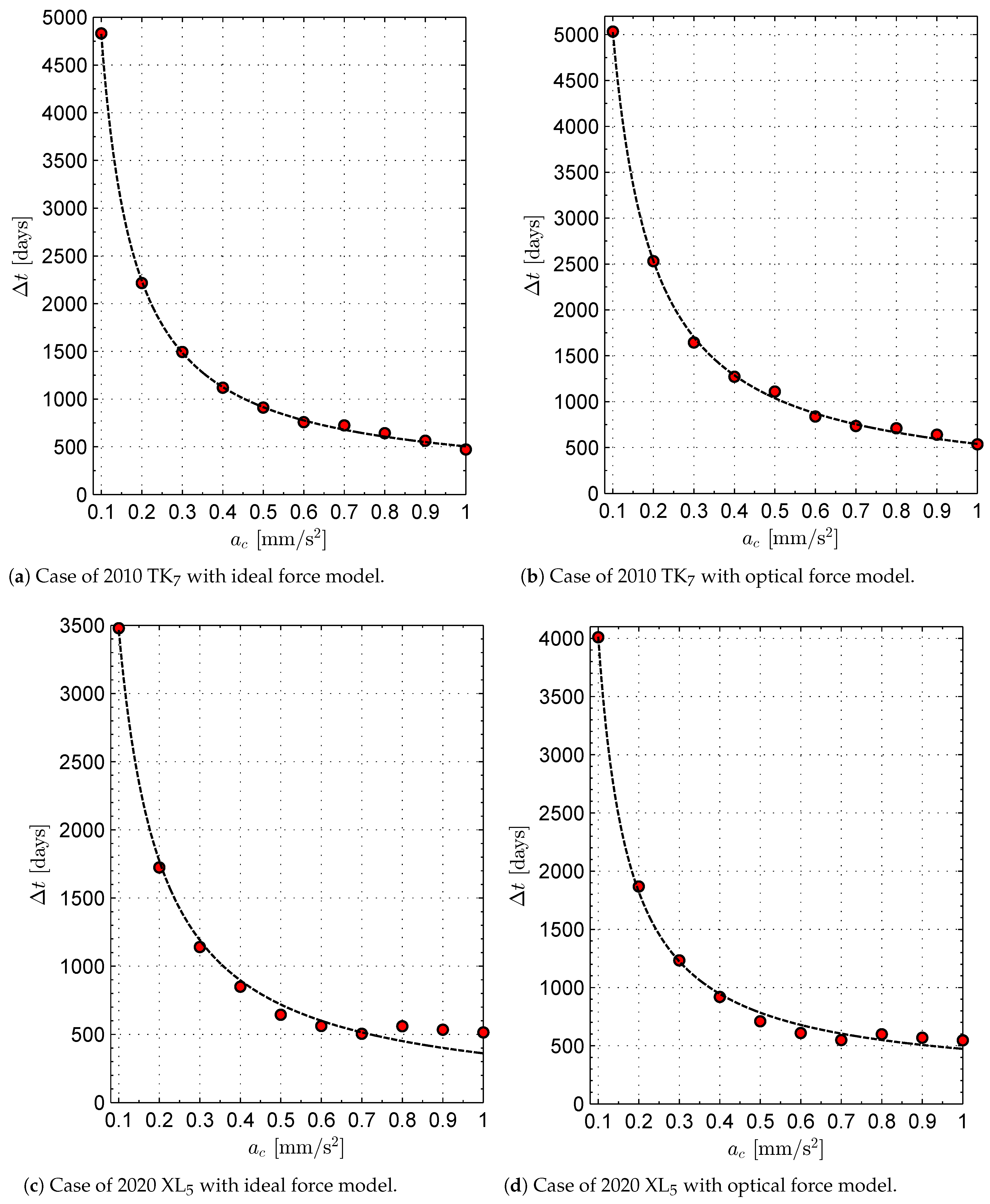
The first two columns of Table 4 and Table 5 can be used, through a best fit procedure, to obtain the function that gives the minimum flight time as a function of the spacecraft characteristic acceleration. For an assigned mission scenario and a given sail force model, the actual variation of the minimum flight time with may be reasonably approximated by the following simple function
where is expressed in days, is in millimeters per square second, and the best fit coefficients are reported in Table 6. Figure 4 shows a comparison between the numerical simulation results and the approximate function given by Equation (47). As expected, when a low characteristic acceleration is considered in the optimization process, the value of N tends to increase (see the last column in Table 4 and Table 5), and the transfer trajectory becomes more involved. This aspect is confirmed by Figure 5, which shows the minimum-time transfer trajectory for the two Earth–ETa mission cases (assuming an optical force model) as a function of the characteristic acceleration .
Case Study
A more detailed analysis is now described in a potential mission scenario from Earth to asteroid 2020 XL, assuming the solar sail to have a propulsive acceleration comparable with that employed in the upcoming NASA’s Solar Cruiser interplanetary mission [31]. Accordingly, a value of and an optical force model have been used in the numerical simulations to obtain the optimal transfer trajectory illustrated in Figure 6. In this case, the optimal flight time is ≃ 3306, whereas Equation (47) estimates an approximate value of about (about smaller). The ephemeris-free optimal orbit-to-orbit transfer starts when the spacecraft true anomaly along the Earth’s orbit is about , whereas the arrival point has a true anomaly (along the ETa heliocentric orbit) of . In this context, the time variations of the classical orbital elements of the spacecraft osculating orbit are shown in Figure 7a. Note that the final values of the elements are consistent with the data reported in Table 3. Finally, the time variations of the three components of the propulsive acceleration vector in the orbital RTN reference frame are sketched in Figure 7b.
4. Conclusions
Minimum-time orbit-to-orbit transfers from Earth to one of the two currently known Trojan asteroids have been simulated by solving an optimal control problem with an indirect approach. For a probe propelled by a (flat) solar sail, feasible trajectories exist that enable those transfers without the need of intermediate planetary flyby. The solar-sail-based spacecraft performance has been investigated with a parametric approach as a function of the spacecraft characteristic acceleration. Using the state-of-the-art level of solar sail technology, the interplanetary transfers require flight times on the order of some years, and a substantial reduction of the transfer time could be reached with a characteristic acceleration of about . In fact, simulations have shown that the mission times tends to drastically decrease as the characteristic acceleration increases to a near-term technology level and, indeed, reduce to about 500 days only when a medium-high performance solar sail (with ) is considered. Although these results have been obtained without considering the planetary ephemerides, they clearly indicate that solar sail propulsion is a very promising option for a mission toward Earth Trojan asteroids. A natural extension of this work is a preliminary analysis of an Earth–ETa transfer by considering the actual planetary ephemerides. Since the two celestial bodies involved in the transfer roughly share the same value of semimajor axis (and so nearly the same orbital period) the ephemeris-constrained transfer can be studied by parametrically analyzing the minimum flight time as a function of the starting true anomaly along the Earth’s orbit, for a fixed value of characteristic acceleration.
Author Contributions
Conceptualization, A.A.Q.; methodology, A.A.Q.; software, A.A.Q.; writing—original draft preparation, A.A.Q. and G.M.; writing—review and editing, G.M. All authors have read and agreed to the published version of the manuscript.
Funding
This work is partly supported by the University of Pisa, Progetti di Ricerca di Ateneo (Grant no. PRA_2022_1).
Institutional Review Board Statement
Not applicable.
Informed Consent Statement
Not applicable.
Data Availability Statement
Not applicable.
Conflicts of Interest
The authors declare no conflict of interest.
Abbreviations
| Notation | |
| a | semimajor axis [au] |
| characteristic acceleration [mm/s] | |
| propulsive acceleration vector [mm/s] | |
| matrix, see Equation (15) | |
| generic entry of matrix , see Equations (16)–(25) | |
| vector, see Equation (14) | |
| non-Lambertian coefficient of the front sail film | |
| non-Lambertian coefficient of the back sail film | |
| force coefficients, see Table 6 | |
| auxiliary vector, see Equation (41) | |
| auxiliary functions, see Equations (43) and (44) | |
| e | eccentricity |
| Hamiltonian function | |
| reduced Hamiltonian function, see Equation (41) | |
| i | orbital inclination [deg] |
| radial unit vector | |
| transverse unit vector | |
| normal unit vector | |
| J | performance index [days] |
| unit vector normal to the sail plane | |
| MEOEs | |
| best fit coefficients, see Equation (47) | |
| r | radial distance [au] |
| Sun–spacecraft unit vector | |
| reference distance [] | |
| t | time [days] |
| spacecraft inertial velocity unit vector | |
| spacecraft state vector | |
| sail cone angle [rad] | |
| flight time [days] | |
| sail clock angle [rad] | |
| emissivity coefficient of the front sail film | |
| emissivity coefficient of the back sail film | |
| adjoint vector, see Equation (39) | |
| generic adjoint variable | |
| Sun’s gravitational parameter [km/s] | |
| argument of periapse [deg] | |
| right ascension of the ascending node [deg] | |
| sail film reflection coefficient | |
| Subscripts | |
| 0 | initial, parking orbit |
| f | final, target orbit |
| Superscripts | |
| · | derivative with respect to time |
References
- Levison, H.F.; Shoemaker, E.M.; Shoemaker, C.S. Dynamical evolution of Jupiter’s Trojan asteroids. Nature 1997, 385, 42–44. [Google Scholar] [CrossRef]
- Almeida, A.J.C.; Peixinho, N.; Correia, A.C.M. Neptune Trojans and Plutinos: Colors, sizes, dynamics, and their possible collisions. Astron. Astrophys. 2009, 508, 1021–1030. [Google Scholar] [CrossRef]
- Trilling, D.E.; Rivkin, A.S.; Stansberry, J.A.; Spahr, T.B.; Crudo, R.A.; Davies, J.K. Albedos and diameters of three Mars Trojan asteroids. Icarus 2007, 192, 442–447. [Google Scholar] [CrossRef] [Green Version]
- Napier, K.J.; Markwardt, L.; Adams, F.C.; Gerdes, D.W.; Lin, H.W. A Collision Mechanism for the Removal of Earth’s Trojan Asteroids. Planet. Sci. J. 2022, 3, 121. [Google Scholar] [CrossRef]
- Mikkola, S.; Innanen, K.A. Studies on solar system dynamics. II - The stability of Earth’s Trojans. Astron. J. 1990, 100, 290–293. [Google Scholar] [CrossRef]
- de la Fuente Marcos, C.; de la Fuente Marcos, R. Transient Terrestrial Trojans: Comparative Short-term Dynamical Evolution of 2010 TK7 and 2020 XL5. Res. Notes AAS 2021, 5, 29. [Google Scholar] [CrossRef]
- Wiegert, P.; Innanen, K.; Mikkola, S. Earth Trojan Asteroids: A Study in Support of Observational Searches. Icarus 2000, 145, 33–43. [Google Scholar] [CrossRef] [Green Version]
- Connors, M.; Wiegert, P.; Veillet, C. Earth’s Trojan asteroid. Nature 2011, 475, 481–483. [Google Scholar] [CrossRef]
- Santana-Ros, T.; Micheli, M.; Faggioli, L.; Cennamo, R.; Devogèle, M.; Alvarez-Candal, A.; Oszkiewicz, D.; Ramírez, O.; Liu, P.Y.; Benavidez, P.G.; et al. Orbital stability analysis and photometric characterization of the second Earth Trojan asteroid 2020 XL5. Nat. Commun. 2022, 13, 447. [Google Scholar] [CrossRef]
- Lei, H.; Xu, B.; Zhang, L. Trajectory design for a rendezvous mission to Earth’s Trojan asteroid 2010 TK7. Adv. Space Res. 2017, 60, 2505–2517. [Google Scholar] [CrossRef]
- Fu, B.; Sperber, E.; Eke, F. Solar sail technology—A state of the art review. Prog. Aerosp. Sci. 2016, 86, 1–19. [Google Scholar] [CrossRef]
- Gong, S.; Macdonald, M. Review on solar sail technology. Astrodynamics 2019, 3, 93–125. [Google Scholar] [CrossRef]
- Zhao, P.; Wu, C.; Li, Y. Design and application of solar sailing: A review on key technologies. Chin. J. Aeronaut. 2022; in press. [Google Scholar] [CrossRef]
- Morrow, E.; Scheeres, D.J.; Lubin, D. Solar Sail Orbit Operations at Asteroids. J. Spacecr. Rocket. 2001, 38, 279–286. [Google Scholar] [CrossRef] [Green Version]
- Mengali, G.; Quarta, A.A. Rapid Solar Sail Rendezvous Missions to Asteroid 99942 Apophis. J. Spacecr. Rocket. 2009, 46, 134–140. [Google Scholar] [CrossRef]
- Dachwald, B.; Seboldt, W.; Richter, L. Multiple rendezvous and sample return missions to near-Earth objects using solar sailcraft. Acta Astronaut. 2006, 59, 768–776. [Google Scholar] [CrossRef]
- Peloni, A.; Ceriotti, M.; Dachwald, B. Solar-Sail Trajectory Design for a Multiple Near-Earth-Asteroid Rendezvous Mission. J. Guid. Control. Dyn. 2016, 39, 2712–2724. [Google Scholar] [CrossRef] [Green Version]
- Song, Y.; Gong, S. Solar-sail trajectory design for multiple near-Earth asteroid exploration based on deep neural networks. Aerosp. Sci. Technol. 2019, 91, 28–40. [Google Scholar] [CrossRef] [Green Version]
- Wright, J.L. Space Sailing; Gordon and Breach Science Publishers: Amsterdam, The Netherlands, 1992. [Google Scholar]
- McInnes, C.R. Solar Sailing: Technology, Dynamics and Mission Applications; Springer: Berlin, Germany, 1999; Chapter 2; pp. 46–53. [Google Scholar] [CrossRef]
- Murphy, D.; Trautt, T. Solar Sail Propulsion Modeling. In Proceedings of the 48th AIAA/ASME/ASCE/AHS/ASC Structures, Structural Dynamics, and Materials Conference, Honolulu, HI, USA, 23–25 April 2007. [Google Scholar] [CrossRef]
- Mengali, G.; Quarta, A.A.; Circi, C.; Dachwald, B. Refined solar sail force model with mission application. J. Guid. Control. Dyn. 2007, 30, 512–520. [Google Scholar] [CrossRef] [Green Version]
- Dachwald, B.; Mengali, G.; Quarta, A.A.; Macdonald, M. Parametric model and optimal control of solar sails with optical degradation. J. Guid. Control. Dyn. 2006, 29, 1170–1178. [Google Scholar] [CrossRef]
- Boni, L.; Mengali, G.; Quarta, A.A. Finite Element Analysis of Solar Sail Force Model with Mission Application. Proc. Inst. Mech. Eng. Part G J. Aerosp. Eng. 2019, 233, 1838–1846. [Google Scholar] [CrossRef]
- Rios-Reyes, L.; Scheeres, D.J. Generalized Model for Solar Sails. J. Spacecr. Rocket. 2005, 42, 182–185. [Google Scholar] [CrossRef] [Green Version]
- Slade, K.; Belvin, K.; Behun, V. Solar Sail Loads, Dynamics, and Membrane Studies. In Proceedings of the 43rd AIAA/ASME/ASCE/AHS/ASC Structures, Structural Dynamics, and Materials Conference, Denver, CO, USA, 22–25 April 2002. [Google Scholar] [CrossRef] [Green Version]
- Li, Q.; Ma, X.; Wang, T. Reduced Model for Flexible Solar Sail Dynamics. J. Spacecr. Rocket. 2011, 48, 446–453. [Google Scholar] [CrossRef]
- Dachwald, B.; Macdonald, M.; McInnes, C.R.; Mengali, G.; Quarta, A.A. Impact of optical degradation on solar sail mission performance. J. Spacecr. Rocket. 2007, 44, 740–749. [Google Scholar] [CrossRef]
- Dachwald, B.; Seboldt, W.; Macdonald, M.; Mengali, G.; Quarta, A.A.; McInnes, C.R.; Rios-Reyes, L.; Scheeres, D.J.; Wie, B.; Görlich, M.; et al. Potential Solar Sail Degradation Effects on Trajectory and Attitude Control. In Proceedings of the AIAA Guidance, Navigation, and Control Conference and Exhibit, San Francisco, CA, USA, 15–18 August 2005. [Google Scholar] [CrossRef] [Green Version]
- Mengali, G.; Quarta, A.A. Optimal three-dimensional interplanetary rendezvous using nonideal solar sail. J. Guid. Control. Dyn. 2005, 28, 173–177. [Google Scholar] [CrossRef]
- Pezent, J.B.; Sood, R.; Heaton, A.; Miller, K.; Johnson, L. Preliminary trajectory design for NASA’s Solar Cruiser: A technology demonstration mission. Acta Astronaut. 2021, 183, 134–140. [Google Scholar] [CrossRef]
- Bassetto, M.; Niccolai, L.; Boni, L.; Mengali, G.; Quarta, A.A.; Circi, C.; Pizzurro, S.; Pizzarelli, M.; Pellegrini, R.C.; Cavallini, E. Sliding mode control for attitude maneuvers of Helianthus solar sail. Acta Astronaut. 2022, 198, 100–110. [Google Scholar] [CrossRef]
- Boni, L.; Bassetto, M.; Niccolai, L.; Mengali, G.; Quarta, A.A.; Circi, C.; Pellegrini, R.C.; Cavallini, E. Structural response of Helianthus solar sail during attitude maneuvers. Aerosp. Sci. Technol. 2023, 133, 108152. [Google Scholar] [CrossRef]
- Walker, M.J.H.; Ireland, B.; Owens, J. A set of modified equinoctial orbit elements. Celest. Mech. 1985, 36, 409–419. [Google Scholar] [CrossRef]
- Walker, M.J.H. Erratum: A set of modified equinoctial orbit elements. Celest. Mech. 1986, 38, 391–392. [Google Scholar] [CrossRef] [Green Version]
- Betts, J.T. Very low-thrust trajectory optimization using a direct SQP method. J. Comput. Appl. Math. 2000, 120, 27–40. [Google Scholar] [CrossRef] [Green Version]
- Betts, J.T. Survey of Numerical Methods for Trajectory Optimization. J. Guid. Control. Dyn. 1998, 21, 193–207. [Google Scholar] [CrossRef] [Green Version]
- Forsythe, G.E.; Malcolm, M.A.; Moler, C.B. Computer Methods for Mathematical Computations; Prentice Hall: Englewood Cliffs, NJ, USA, 1976. [Google Scholar]
- Bate, R.R.; Mueller, D.D.; White, J.E. Fundamentals of Astrodynamics; Dover Publications: New York, NY, USA, 1971; Chapter 2; pp. 53–55. [Google Scholar]
- Bryson, A.E., Jr.; Ho, Y.C. Applied Optimal Control; Hemisphere Publishing Corporation: New York, NY, USA, 1975. [Google Scholar]
- Stengel, R.F. Optimal Control and Estimation; Dover Publications: Mineola, NY, USA, 1994; pp. 222–254. [Google Scholar]
Figure 1.
Solar sail propulsive acceleration direction and cone angle.

Figure 2.
Sail cone () and clock () angles.

Figure 3.
Variation of with the cone and clock angle in an exemplary case.

Figure 4.
Simulation results (red circle) and best fit interpolation (dashed black line) of the flight time as a function of the characteristic acceleration.
Figure 4.
Simulation results (red circle) and best fit interpolation (dashed black line) of the flight time as a function of the characteristic acceleration.

Figure 5.
Optimal Earth–ETa transfer trajectory (black line), assuming an optical force model, as a function of the characteristic acceleration. Blue line → Earth’s orbit, red line → asteroid orbit, blue circle → start, red circle → arrival, blue star → Earth’s orbit perihelion, red star → asteroid orbit perihelion, yellow circle → Sun.

Figure 6.
Optimal trajectory in an Earth–asteroid 2020 XL transfer, with and an optical force model. The figure legend is consistent with that reported in the label of Figure 5.
Figure 6.
Optimal trajectory in an Earth–asteroid 2020 XL transfer, with and an optical force model. The figure legend is consistent with that reported in the label of Figure 5.

Figure 7.
Time variation of the osculating orbit elements and propulsive acceleration components (in an RTN reference frame) in an Earth–asteroid 2020 XL transfer, with and an optical force model. Blue circle → start; red circle → arrival.
Figure 7.
Time variation of the osculating orbit elements and propulsive acceleration components (in an RTN reference frame) in an Earth–asteroid 2020 XL transfer, with and an optical force model. Blue circle → start; red circle → arrival.


Table 1.
Reflective film optical coefficients in an ideal case, and in a sail membrane with a highly reflective aluminum coated front side and a highly emissive chromium-coated backside.
Table 1.
Reflective film optical coefficients in an ideal case, and in a sail membrane with a highly reflective aluminum coated front side and a highly emissive chromium-coated backside.
| Force Model | s | |||||
|---|---|---|---|---|---|---|
| ideal | 1 | 1 | 0 | 0 | ||
| optical |
Table 2.
Force coefficients for an ideal and an optical force model obtained through Equations (3)–(5).
Table 2.
Force coefficients for an ideal and an optical force model obtained through Equations (3)–(5).
| Force Model | |||
|---|---|---|---|
| ideal | 0 | 2 | 0 |
| optical |
Table 3.
Classical orbital elements used in the numerical simulations.
| Celestial Body | a [au] | e | i [deg] | [deg] | [deg] |
|---|---|---|---|---|---|
| Earth | |||||
| 2010 TK | |||||
| 2020 XL |
Table 4.
Earth–asteroid 2010 TK minimum-time performance as a function of the characteristic acceleration and the sail force model.
Table 4.
Earth–asteroid 2010 TK minimum-time performance as a function of the characteristic acceleration and the sail force model.
| [mm/s] | Force Model | [Days] | [deg] | [deg] | N |
|---|---|---|---|---|---|
| 0.1 | optical | 5032.8 | 280.3 | 196.2 | 15 |
| 0.1 | ideal | 4830.9 | 264.4 | 214.3 | 13 |
| 0.2 | optical | 2530.9 | 281.1 | 193.9 | 7 |
| 0.2 | ideal | 2215.7 | 306.3 | 158.3 | 7 |
| 0.3 | optical | 1644.5 | 311.3 | 154.2 | 5 |
| 0.3 | ideal | 1494.0 | 347.3 | 129.7 | 5 |
| 0.4 | optical | 1271.4 | 284.5 | 188.2 | 3 |
| 0.4 | ideal | 1119.3 | 304.6 | 160.1 | 3 |
| 0.5 | optical | 1110.7 | 266.8 | 245.0 | 3 |
| 0.5 | ideal | 910.2 | 291.8 | 176.5 | 2 |
| 0.6 | optical | 838.4 | 306.4 | 155.6 | 2 |
| 0.6 | ideal | 758.4 | 318.6 | 133.5 | 2 |
| 0.7 | optical | 733.8 | 336.4 | 126.3 | 2 |
| 0.7 | ideal | 723.9 | 291.0 | 276.3 | 2 |
| 0.8 | optical | 710.1 | 317.5 | 289.9 | 2 |
| 0.8 | ideal | 643.3 | 5.2 | 286.5 | 1 |
| 0.9 | optical | 640.4 | 32.2 | 278.5 | 1 |
| 0.9 | ideal | 564.4 | 110.5 | 279.0 | 1 |
| 1 | optical | 535.1 | 86.7 | 189.6 | 1 |
| 1 | ideal | 471.4 | 103.8 | 168.0 | 1 |
Table 5.
Earth–asteroid 2020 XL minimum-time performance as a function of the characteristic acceleration and the sail force model.
Table 5.
Earth–asteroid 2020 XL minimum-time performance as a function of the characteristic acceleration and the sail force model.
| [mm/s] | Force Model | [Days] | [deg] | [deg] | N |
|---|---|---|---|---|---|
| 0.1 | optical | 4008.9 | 150.5 | 195 | 12 |
| 0.1 | ideal | 3478.8 | 213.8 | 119.5 | 11 |
| 0.2 | optical | 1868.1 | 195.2 | 127.2 | 6 |
| 0.2 | ideal | 1724.2 | 224.9 | 116.2 | 6 |
| 0.3 | optical | 1233.4 | 205.5 | 122.2 | 4 |
| 0.3 | ideal | 1140.7 | 237.4 | 113.2 | 4 |
| 0.4 | optical | 919 | 214.0 | 119.1 | 3 |
| 0.4 | ideal | 849.6 | 245.4 | 112.0 | 3 |
| 0.5 | optical | 710.2 | 185.1 | 132.4 | 2 |
| 0.5 | ideal | 643.7 | 205.6 | 119.0 | 2 |
| 0.6 | optical | 608.6 | 228.0 | 113.4 | 2 |
| 0.6 | ideal | 561.6 | 256.8 | 108.4 | 1 |
| 0.7 | optical | 547.9 | 282.2 | 110.2 | 1 |
| 0.7 | ideal | 504.3 | 337.5 | 111.1 | 1 |
| 0.8 | optical | 598 | 225.0 | 292.8 | 1 |
| 0.8 | ideal | 559.6 | 246.7 | 286.6 | 1 |
| 0.9 | optical | 568.2 | 248.2 | 292.1 | 1 |
| 0.9 | ideal | 533.8 | 272.0 | 285.3 | 1 |
| 1 | optical | 546.6 | 269.3 | 290.8 | 1 |
| 1 | ideal | 514.7 | 294.9 | 283.6 | 1 |
Table 6.
Best fit coefficients in Equation (47) as a function of the mission scenario and the sail force model.
Table 6.
Best fit coefficients in Equation (47) as a function of the mission scenario and the sail force model.
| Scenario | Force Model | ||||
|---|---|---|---|---|---|
| Earth-2010 TK | ideal | 12,285 | 41,589 | ||
| Earth-2010 TK | optical | 6648 | |||
| Earth-2020 XL | ideal | ||||
| Earth-2020 XL | optical | 3738 |
Disclaimer/Publisher’s Note: The statements, opinions and data contained in all publications are solely those of the individual author(s) and contributor(s) and not of MDPI and/or the editor(s). MDPI and/or the editor(s) disclaim responsibility for any injury to people or property resulting from any ideas, methods, instructions or products referred to in the content. |
© 2023 by the authors. Licensee MDPI, Basel, Switzerland. This article is an open access article distributed under the terms and conditions of the Creative Commons Attribution (CC BY) license (https://creativecommons.org/licenses/by/4.0/).
Share and Cite
MDPI and ACS Style
Quarta, A.A.; Mengali, G. Solar Sail Trajectories to Earth’s Trojan Asteroids. Universe 2023, 9, 186. https://doi.org/10.3390/universe9040186
AMA Style
Quarta AA, Mengali G. Solar Sail Trajectories to Earth’s Trojan Asteroids. Universe. 2023; 9(4):186. https://doi.org/10.3390/universe9040186
Chicago/Turabian StyleQuarta, Alessandro A., and Giovanni Mengali. 2023. "Solar Sail Trajectories to Earth’s Trojan Asteroids" Universe 9, no. 4: 186. https://doi.org/10.3390/universe9040186
Note that from the first issue of 2016, this journal uses article numbers instead of page numbers. See further details here.