Article

On Warm Natural Inflation and Planck 2018 Constraints

by
Mahmoud AlHallak
1,†,
Khalil Kalid Al-Said
2,†,
Nidal Chamoun
3,*,† and
Moustafa Sayem El-Daher
4,5,†
1
Physics Department, Damascus University, Damascus P.O. Box 30621, Syria
2
Physics Department, University of Doha for Science and Technology, Doha P.O. Box 24449, Qatar
3
Physics Department, HIAST, Damascus P.O. Box 31983, Syria
4
Higher Institute of Laser Applications and Researches, Damascus University, Damascus P.O. Box 30621, Syria
5
Faculty of Informatics and Communications, Arab International University, Daraa 4076, Syria
*
Author to whom correspondence should be addressed.
These authors contributed equally to this work.
Universe 2023, 9(2), 80; https://doi.org/10.3390/universe9020080
Submission received: 14 November 2022 / Revised: 20 January 2023 / Accepted: 24 January 2023 / Published: 2 February 2023
(This article belongs to the Special Issue Warm Inflation)

Abstract

:
We investigate natural inflation with non-minimal coupling to gravity, characterized either by a quadratic or a periodic term, within the warm inflation paradigm during the slow-roll stage, in both strong and weak dissipation limits; and show that, in the case of a T-linearly dependent dissipative term, it can accommodate the spectral index n s and tensor-to-scalar ratio r observables given by Planck 2018 constraints, albeit with a too-small value of the e-folding number to solve the horizon problem, providing, thus, only a partial solution to natural inflation issues, assuming a T-cubically dependent dissipative term can provide a solution to this e-folding number issue.
PACS:
98.80Cq; 98.80-k

1. Introduction

Inflationary cosmology [1,2] is now the dominant perspective for explaining the early universe’s physics, solving the flatness and homogeneity/unwanted relics problems, and providing a mechanism to interpret the inhomogeneities in the cosmic microwave background radiation (CMBR). In the standard slow-roll cold inflation models, the universe experiences an exponential expansion, during which density perturbations are created by quantum fluctuations of the inflation field, followed by the reheating stage, where a temporarily localized mechanism must rapidly distribute sufficient vacuum energy.
Fang and Berera [3] realized that by combining the exponential accelerating expansion phase and the reheating, one could resolve disparities assembled by each separately. In [4], Berbera proposed a warm inflationary model in which thermal equilibrium is maintained during the inflationary phase and radiation production is started throughout it; i.e., relativistic particles are created during the inflationary period.
Many inflationary models inspired by particle physics, string theory, and quantum gravity have been studied within the context of warm inflation. Visinelli [5] derived and analyzed the experimental bounds on warm inflation with a monomial potential, whereas Kamali in [6] investigated the warm scenario with non-minimal coupling (NMC) to gravity with a Higgs-like potential. Warm inflation was constrained by CMB data in [7]. The authors of [8] treated the warm scenario with NMC through modified gravity with a special potential motivated by variation of constants. In [9], warm inflationary models in the context of a general scalar-tensor theory of gravity were investigated within only the strong limit of dissipation.
The natural inflation (NI) proposed by Freese, Frieman, and Olinto [10], with a cosine potential, is a popular model due to its shift symmetry with a flat potential, preventing significant radiative corrections from being introduced, which gives NI an ability to solve theoretical challenges inherent in slow-rolling inflation models. However, NI is disfavored at greater than the 95 % confidence level by current observational constraints from P l a n c k 2018 of the scalar-tensor ratio r and spectral index n s [11,12]. Moreover, a more recent analysis of BICEP/Keck XIII in 2018 (BK18) [13] has put more stringent bounds on r, whereas the authors of [14] discussed a way to amend the discrepancies of NI with data by non-minimally coupling the scalar fields to the Starobinski model ( f ( R ) ) in the Palatini formalism. In [15], it was shown that NMC to gravity within the f ( R ) setting was enough to bring “cold” NI to within 95 % confidence levels of the current observational constraints represented by P l a n c k 2018 (TT, EE, TE), BK18, and other experiments (lowE, lensing), separately or combined.
The study of warm NI was pioneered by Visinelli [16], and separately, by [17], and then pursued by many others, such as [18]. When applied to primordial black holes (gravitational waves), the setup was analyzed in many articles, say [19,20,21,22,23].
The aim of this work was to study NI with NMC to gravity within the warm paradigm, in both the strong and weak limits of the dissipation term characterizing the warm scenario. We study two forms for the NMC to the gravity term, which is generally produced at one-loop order in the interacting theory for a scalar field, even if it is absent at the tree level [24]. Actually, in general, all terms of the form ( R i ϕ j , R μ ν μ ϕ ν ϕ , ) are allowed in the action. However, omitting the derivative terms and taking a finite number of loop graphs enforce a polynomial form of the NMC term, and if one imposes CP symmetry on the action, the term should include even powers of the inflaton field ϕ . For simplicity, we include only the quadratic monomial ( ξ ϕ 2 R ) of dim-4. However, since some microscopic theories may suggest the emergence of an NMC similar in the form of the original potential [25], we also consider an NMC of a periodic form respecting the shift symmetry of the NI potential, making it of the form ( λ 1 + cos ( ϕ f ) ).
We find that the NI with NMC to gravity within the warm paradigm, in the case of a linear dissipative term, is able to accommodate the ( n s , r ) observable constraints, but at the price of getting a small value for the e-folding number N e 30 to solve the horizon and flatness problems. However, one can make N e acceptable (≥40), in this T-linearly dependent regime, but for n s 0.98 , just getting outside the admissibility contours. Studying the case of T-cubically dependent dissipative term gave in the strong limit scenario some benchmarks which satisfy the four constraints of n s , r , A s and N e in both cases of quadratic or periodic non-minimal coupling to gravity.
The paper is organized as follows. In Section 2, we present the setup of the warm paradigm, for general potentials, whereas in Section 3 we specify the study to NI. In Section 4 and Section 5, we study the strong (weak) limit ( Q Γ 3 H > > ( < < ) 1 ) for both quadratic and periodic NMC. In Section 6, we study briefly the strong limit scenario when the dissipative term is proportional to the cubic power of the temperature, whereas we end up with conclusions and a summary in Section 7.

2. Warm Inflation Setup

2.1. Arena

We consider the general local action for a scalar field coupled with radiation and gravity within the Jordan frame:
S = d 4 x g 1 2 Ω 2 ( ϕ ) R + L ϕ + L γ + L I n t .
where g is the determinant of the metric g μ ν , L γ is the Lagrangian density of the radiation field and L I n t describes the interaction between the latter and the inflaton ϕ , whose Lagrangian density, considered as that of a canonical scalar field, is given by
L ϕ = 1 2 g μ ν Δ μ ϕ Δ ν ϕ V ( ϕ ) ,
where V ( ϕ ) is the inflaton potential, whereas Ω 2 ( ϕ ) indicates the NMC between the scalar field ϕ and the gravity described by the usual Einstein–Hilbert action rather than the Starobinski f ( R ) gravity.
One can take the usual electromagnetic Lagrangian for L γ , while we leave aside, for now, the “unknown” interaction density L I n t . By carrying out the usual action, optimization, by changing with respect to metric and approximating the energy-momentum tensor for both the inflaton and the radiation fields by perfect fluids characterized by energy density ρ and pressure p, we get the following equation of motion:
ρ ˙ ϕ + 3 H ρ ϕ + p ϕ + 1 2 ( Ω 2 ) ϕ ϕ ˙ R + ρ ˙ γ + 4 H ρ γ = 0 ,
with ( Ω 2 ) ϕ meaning a derivative with respect to ϕ . Some remarks are in order here. First, the two terms—including the Hubble constant “H” terms, which are known to be related to “total energy”, both that of radiation and that of the inflaton—represent a “direct” coupling between the inflaton and radiation, in contrast to the “indirect” one via the gravity, which couples to all fields. Second, L i n t contributes an additional “direct” coupling. However, we still assume that its contribution to the total energy density is negligible, such that
ρ t o t = ρ ϕ + ρ γ
There are in the literature some microscopic models for L i n t (look for, e.g., [9]), but we shall not dwell on their details, but rather assume that its effect is described phenomenologically by a term Γ ϕ ˙ 2 , which can be motivated/justified in a field theory approach specific to the considered microscopic model. As a matter of fact, the Γ factor embodies the microscopic physics resulting from the interaction between ϕ and other particles, where ϕ can usually be assumed to couple to heavy intermediate fields that, in their turn, couple to light radiation fields. As ϕ rolls slowly on its potential, it triggers the decay of the heavy fields into the light ones, thereby generating a dissipative term [26,27]. Another method adopted in warm scenarios is where ϕ is a Goldstone boson coupled directly to the light radiation, but gets protected from large thermal corrections due to a symmetry imposed on the model [26,28]. A supersymmetric model was studied in [29], whereas [30] conceived a model, which is also supersymmetric, leading to a dissipative factor of the form Γ T m ϕ m 1 .
We thus assume that these microscopic models lead to a phenomenological term such that:
ρ ˙ γ + 4 H ρ γ = Γ ϕ ˙ 2
whence from Equation (3) we have
ρ ˙ ϕ + 3 H ρ ϕ + p ϕ + 1 2 ( Ω 2 ) ϕ ϕ ˙ R = Γ ϕ ˙ 2
Using
ρ ϕ = 1 2 ϕ ˙ 2 + V , p ϕ = 1 2 ϕ ˙ 2 V
we get
ϕ ¨ + 3 H ϕ ˙ V ϕ + 1 2 ( Ω 2 ) ϕ R = Γ ϕ ˙
Actually, although this “friction” term Γ ϕ ˙ , describing phenomenologically the decay of ϕ , may be inadequate to describe the energy transfer from ϕ from far out of the equilibrium; it is however, suitable to describe the energy dissipated by ϕ into a thermalized radiation bath [3]. We shall not discuss the nature of these particles into which ϕ decays [31,32]; rather, we approximate them by thermal radiation (namely, of photons) such that energy is still dominated by ϕ , and fluctuations are dominated by thermal, not quantum, ones.
We can see that Equation (3) expresses the conservation of total energy, in which one neglects the contribution of L i n t , which, meanwhile and through Equations (5) and (6), affects individually both ρ γ and ρ ϕ . There are many possibilities for the dissipative term, but we shall study in this article mainly the case where it depends linearly on temperature ( Γ = Γ 0 T ), whereas we briefly study in the penultimate section the case of cubical dependence on temperature ( Γ = Γ 0 T 3 ).
During warm inflation, we have T H , and due to the inflaton interactions with the matter/radiation, a bath of particles is continuously produced during the slow-roll period, which transits the universe into a radiation-dominated phase through eliminating of a smooth transition, hence the need for a reheating stage. Thermal fluctuations dominate over quantum fluctuations, even though ρ γ is neglected compared to ρ ϕ , which is reflected through the factor
Q = Γ 3 H = Γ 0 T 3 H ,
so that the inflation is described to be in the strong (weak) limit regime when Q 1 ( Q 1 ).
It is convenient to go from the Jordan frame to the Einstein frame, in which the gravitational sector of the action takes the form of the Hilbert–Einstein action, and the NMC to gravity disappears. Consequently, in the Einstein frame, one is able to use the usual equations of general relativity, the inflationary solutions, and the standard slow-roll analysis.
The conformal transformation is defined as:
g ˜ μ ν = Ω 2 ( ϕ ) g μ ν g ˜ = Ω 4 g
leading to the action expressed in the Einstein frame by
S = d 4 x g ˜ 1 2 R ˜ 1 2 1 + 6 ( Ω ) 2 Ω 2 g ˜ μ ν ˜ μ ϕ ˜ ν ϕ V ( ϕ ) Ω 4 + d 4 x g ˜ L ˜ γ + S I n t .
For the radiation field, and since the corresponding integrand in the action is invariant under rescaling, by Equation (10) we find that the Lagrangian density (energy-momentum tensor) is divided by Ω 4 ( Ω 2 ) as:
T μ ν γ = 2 g δ g L γ δ g μ ν T ˜ μ ν γ = 2 g δ g ˜ L ˜ γ δ g ˜ μ ν = T μ ν γ Ω 2 ,
and thus we conclude that the perfect fluid assumption for the radiation field will remain valid in the Einstein frame with energy density ( ρ γ = ρ γ Ω 4 ) and pressure ( p γ = p γ Ω 4 ). Taking the definition of temperature:
ρ ( γ ) γ = C γ T ( γ ) γ 4 : C γ = π 2 g * 30 ,
with g * denoting the number of created massless modes, we see that the temperature scales by 1 / Ω going from the Jordan to the Einstein frame:
T J o r d a n E i n s t e i n T / Ω
As to the inflaton and gravity sector, we see that in the Einstein frame, there is a “pure” GR gravity part, whereas we have a non-canonical kinetic term for the inflaton scalar field, which can be put in a canonical form by defining a new field χ , related to ϕ by:
d ϕ d χ 2 1 Z 2 = Ω 2 1 + 6 ( Ω ϕ ) 2 = 2 Ω 4 2 Ω 2 + 3 ( ( Ω 2 ) ϕ ) 2 ,
so to get (from now on, we drop the tilde off, but we keep in mind that all calculations are carried out in the Einstein frame):
S = d 4 x g 1 2 R 1 2 g μ ν μ χ ν χ U ( χ ) + S γ + S I n t ,
where
U ( χ ) = V ( ϕ ( χ ) ) Ω 4
A spatially flat Friedmann–Robertson–Walker (FRW) universe gives the energy density ρ χ and the pressure p χ of the inflaton field as
ρ χ = 1 2 χ ˙ 2 + U ( χ ) , p χ = 1 2 χ ˙ 2 U ( χ )
with Friedman equation given by
H 2 = 1 3 ρ t o t = 1 3 ( ρ χ + ρ γ ) .
For the interaction Lagrangian L i n t , and while lacking a model-independent Lagrangian term leading to the RHS of (8), we shall argue by comparison to the cold inflation scenario in order to find the corresponding equation in the Einstein frame. Note that, unlike standard studies [6] where the damping term is introduced in the Einstein frame, we espouse the viewpoint that the field approach models justifying the damping term form are to be defined in the original Jordan frame. However, we shall show that under an approximation, which we shall adopt, the form would be similar in the two frames. Actually, the Hubble parameter transformation has an inhomogenous term [33]1:
H J o r d a n E i n s t e i n H / Ω + log Ω ˙ Ω ;
then, by looking at Equation (14) and dropping/neglecting the inhomogeneous logarithmic variation of Ω , we can see that T H is conformally invariant, and likewise, the factor Q (Equation 9) is also invariant. In the Einstein frame, the field will undergo slow-roll generation of inflation where one assumes approximate constancy for both H and T [29], so one can consider Q as constant in the Einstein frame, and thus also in the Jordan frame. We know that in cold inflation, including NMC to gravity, a Jordan-frame Euler–Lagrange-type equation expressing metric stationarity:
ψ ¨ J + 3 H J ψ ˙ J + ( V J ) ψ J + 1 2 ( Ω 2 ) ψ J R = 0
would lead in the Einstein frame to a standard GR inflationary equation:
ψ ¨ E + 3 H E ψ ˙ E + ( V E ) ψ E = 0
We see now that using Equation (9) in Equation (8), we get an equation similar to Equation (21), but with ( 3 H J ) replaced by ( 3 ( 1 + Q ) H J ) , where Q is approximately constant. Then, we conclude that we get in the Einstein frame an equation similar to Equation (22) with ( H E ) replaced by ( H E ( 1 + Q ) ). By rewriting Q in the Einstein frame, we get (dropping the subscript E) in the Einstein frame:
χ ¨ + 3 H χ ˙ + U χ = Γ χ ˙ = Γ 0 T χ ˙
The upshot here is that we can use, under some approximation and for a damping factor linearly proportional to temperature, the above standard form, albeit starting from a free parameter Γ 0 defined originally in the Jordan frame. By conservation of energy, we get:
ρ ˙ γ + 3 H ( ρ γ + p γ ) = ρ ˙ γ + 4 H ρ γ = + Γ χ ˙ 2
The fundamental equations for warm inflation within the slow-roll approximation ( χ ˙ 2 U , χ ¨ χ ˙ , ρ ˙ γ ρ γ ) are:
H 2 U / 3 , H ˙ 1 2 ( 1 + Q ) χ ˙ 2 ,
ρ γ 3 4 Q χ ˙ 2 , χ ˙ U χ 3 H ( 1 + Q ) .
Using Equation (13), we get
T = 1 4 C γ Q ( 1 + Q ) 2 ( U χ ) 2 U 1 4

2.2. Power Spectrum

We define the following slow-roll parameters:
ϵ = 1 2 U χ U 2 = Z 2 ϵ ϕ ,
η = U χ χ U = Z 2 η ϕ + Z Z ϕ 2 ϵ ϕ ,
β = Γ χ U χ Γ U = Z 2 β ϕ ,
where ϵ ϕ , η ϕ , β ϕ correspond to the same definitions with the derivative carried out with respect to the field ϕ . One can show that the slow-roll regime is met provided we have
ϵ , η , β 1 + Q
The spectrum of the adiabatic density perturbations generated during inflation given by [6] (the star * parameter denotes parameter at horizon crossing):
Δ R ( k ) = A s k k * n s ( k ) 1 = P 0 ( k / k * ) F ( k / k * ) :
P 0 ( k / k * ) = H * 2 2 π χ ˙ k 2 , F ( k / k * ) = 1 + 2 ν k + ω k G ( Q * ) :
ν k = 1 e H T 1 , ω k = T H 2 3 π Q k 3 + 4 π Q k ,
A s = Δ R ( k * ) = H * 2 2 π χ ˙ k * 2 1 + 2 ν k * + ω k * G ( Q * ) ,
where A s represents the amplitude of the CMB fluctuations at the scale k * , and where the modification function G, which is due to coupling between the inflaton field and radiation fluctuations, is given numerically for a linearly T-dependent dissipation by:
G ( Q ) = 1 + 0.335 Q 1.364 + 0.0815 Q 2.315 .
The curvature perturbation spectrum has been measured by PLANCK (WMAP) at the 68 % confidence level at the fixed wave number k = 0.05 ( 0.002 ) Mpc 1 as [35,36]
A s [ 2.136 , 2.247 ] × 10 9 , [ 2.349 , 2.541 ] × 10 9
and thus the model seeks to reproduce these observational constraints, or at least to reproduce their order of magnitude ( 10 9 ).
We see that the cold inflation is restored when ( ν k ), the Bose–Einstein distribution in a radiation bath of temperature T, and ω k , due to thermal effects, all go to zero:
ν k 0 & ω k 0 cold   inflation
The observable spectral index is given by:
n s 1 = d log Δ R ( k ) d log k k = k * = 1 H d log Δ R ( k ) d t = 1 H Δ R d Δ R d t
whereas the observable r, the tensor-to-scalar ratio, is given by:
r = Δ T ( k ) Δ R = 2 H 2 π 2 Δ R = 16 ϵ ( 1 + Q ) 2 F 1
We distinguish two limit regimes.
  • Strong Limit Q 1 :
    Here, using Equation (27), one can show that
    T = Z 2 ( U ϕ ) 2 4 H C γ Γ 0 1 / 5
    We have via Equation (34):
    ω k = T π Γ H 3 = T H 3 π Q
    Thus, 1 + ν k T H ω k , and one gets:
    Δ R = Δ R s G : Δ R s = 3 T H 8 π ϵ 2 Q 5 2
    Thus, we get
    n s 1 = 1 H Δ R s d Δ R s d t + Q ˙ H G Q G
    The first term will give, after lengthy calculations look at [5]:
    1 H Δ R s d Δ R s d t = 1 Q 9 4 ϵ + 3 2 η 9 4 β
    whereas we get for the second term:
    Q ˙ H G Q G = 2.315 Q ( ϵ β )
    where we have used the identity:
    Q ˙ H Q = Γ ˙ H Γ H ˙ H 2 = 1 1 + Q ( β ϵ )
    Thus, we get:
    n s 1 = 1 Q 9 4 ϵ + 3 2 η 9 4 β + 2.3 ϵ 2.3 β
    Note that n s involves the temperature T through the expression of Q = Γ 0 T 3 H . Additionally, T plays a role in determining the “end of inflation” field, ϕ f being the argument of the slow-roll parameter ( ϵ , η , β ) when it equals 1 + Q = 1 + Γ 0 T 3 H , whichever among the three meets the equality first. Determining ϕ f allows one to compute the e-folding number by:
    N e log a e n d a k = t t f H d t = χ k χ f H d χ χ ˙ χ f χ k U U χ ( 1 + Q ) d χ = ϕ f ϕ k U U ϕ ( 1 + Q ) Z 2 d ϕ
    The initial time when the inflation started is taken to correspond to the horizon crossing when the dominant quantum fluctuations freeze, transforming into classical perturbations with observed power spectrum.
    As for the tensor-to-scalar ratio, we get
    r = H T 16 ϵ Q 5 / 2 G 1 = H T 16 ϵ 0.0185 Q 4.815
  • Weak Limit Q 1
    Using Equation (27), one can show that
    T = Z 2 ( U ϕ ) 2 Γ 0 36 C γ H 3 1 / 3
    From Equation (34), we have
    ω k = 2 π Γ T 3 H 2 = 2 π T Q H
    Thus, 1 + ν k T H ω k , and one gets:
    Δ R = Δ R w G : Δ R w = 4 T H π ϵ 2
    Thus, we get
    n s 1 = 1 H Δ R w d Δ R w d t + Q ˙ H G Q G
    The first term will give, after lengthy calculations look at [5]:
    1 H Δ R w d Δ R w d t = 1 6 ϵ + 2 η + ω k 1 + ω k 15 ϵ 2 η 9 β 4
    which gives, under the condition:
    ω k = 2 π T Q H 1 ,
    the answer
    1 H Δ R w d Δ R w d t = 1 6 ϵ + 2 η + 2 π Γ 0 T 2 3 H 2 15 ϵ 2 η 9 β 4
    As to the second term, we get using Equation (47)
    Q ˙ H G Q G = 0.456 Q 1.364 ( ϵ β )
    Thus, we get:
    n s 1 = 1 6 ϵ + 2 η + 2 π Γ 0 T 2 12 H 2 ( 15 ϵ 2 η 9 β ) + 0.456 Q 1.364 ( ϵ β )
    As for the tensor-to-scalar ratio, we get, using G 1 , the following:
    r = 16 ϵ ( 1 + Q ) 2 F 1 = 8 H ϵ T = 8 H Z 2 ϵ ϕ T

3. Natural Inflation

The potential in the NI is periodic of the form
V = V 0 1 + cos ( ϕ f )
where V 0 is a scale of an effective field theory generating this potential, and f is a symmetry breaking scale. As mentioned in the introduction, we shall consider two well-motivated forms of NMC to gravity:
  • Quadratic NMC:
    Ω 2 ( ϕ ) = 1 + ξ ϕ 2
    which is considered a leading order of terms allowed in the action generated by loops in the interacting theory. ξ is the free parameter coupling constant characterizing the strength of the NMC to gravity.
  • Periodic NMC
    Ω 2 ( ϕ ) = 1 + λ 1 + cos ( ϕ f )
    which is similar in form to the original potential, allowing it to be justified in some microscopic models.
It is well known that cold natural inflation with NMC is not enough to accommodate data. In [15], we showed that cold natural inflation with NMC and F ( R ) -modified gravity was viable. Here, we are trying to dispense with the modification of the gravity ingredient, while assuming, instead, the warm scenario. We shall see that two constraints out of three can be met for the warm NI with NMC.
The strategy would amount to carrying out an exhaustive scan of the free-parameters space (that of ϕ * , Γ 0 , f , V 0 , ξ or λ ) and computing for each “benchmark” the corresponding n s , r and ϕ f , the latter making one of the slow parameters equal to ( 1 + Q ) , which would allow us to compute the e-folding number N e , which with ( n s , r ) would constitute the observational constraints to be accommodated. As to the number of relativistic degrees of freedom of radiation, we use g * ( T ) = 228.75 , i.e., C γ = 75.2557 , corresponding to the number of relativistic degrees of freedom in the minimal supersymmetric standard model at temperatures greater than the electroweak phase transition.

4. Comparison to Data: Strong Case
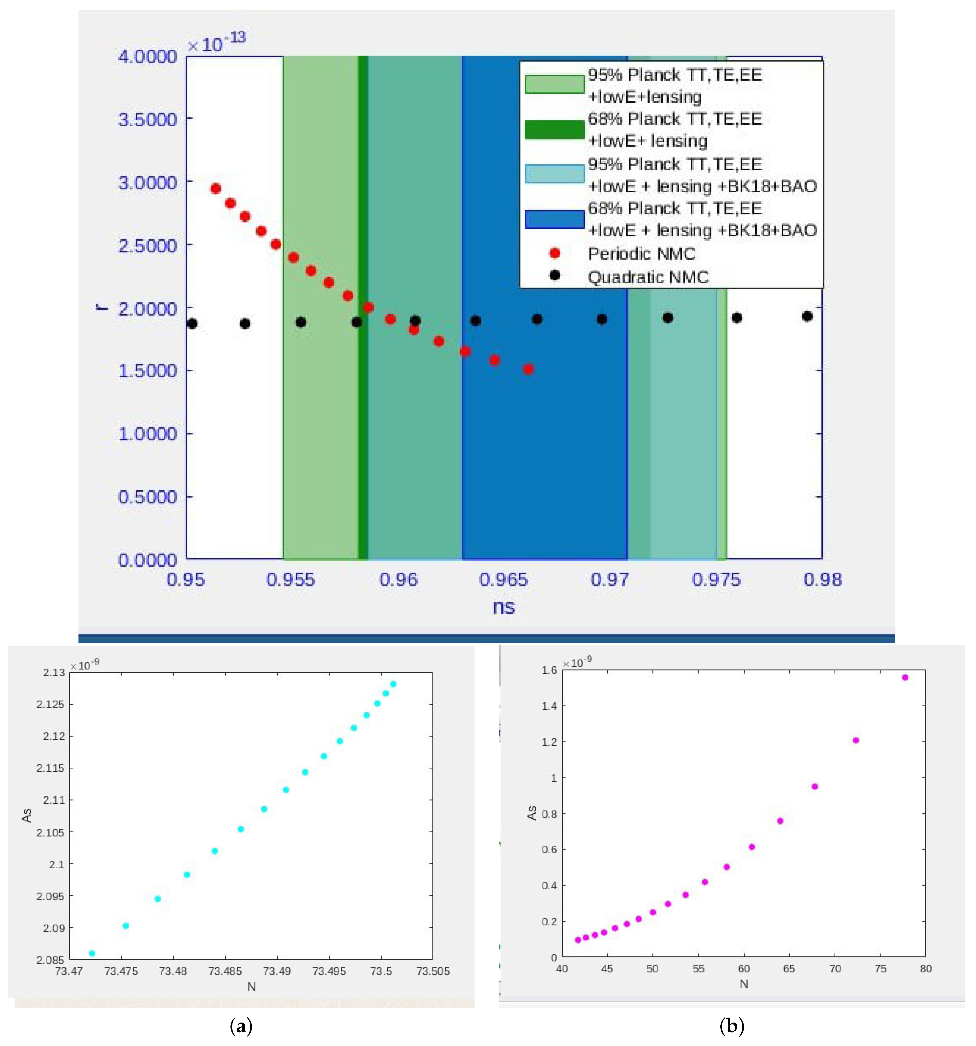
We carried out an extensive scan over the free-parameters space, and for each point we computed ( n s , r ) and N e . We could not find benchmarks meeting the constraints of ( n s , r ) at the 95 % confidence level according to the 2018 Planck (TT, EE, TE), BK18, and other experiments (lowE, lensing) separately or combined, which would allow also for acceptable N e 40 in order to solve the flatness and horizon problems. Accommodating ( N e = 40 , r ) was possible, but at the expense of getting a somewhat large ( n s ).
  • Quadratic NMC
    Figure 1 shows the results of scanning the parameters space in the case of strong-limit warm NI with quadratic NMC to gravity. One could accommodate ( n s , r ) but with too little N e . In the figures, the two colors dots correspond to two choices of the coupling ξ = 20 , 40 .
    Looking to meet the e-folds constraint, we imposed ( N e = 40 ) with ( ξ = 20 ), and fixed the values of ( Γ 0 , f , V 0 ) as before, while scanning over ϕ * . We found the “bench mark”: ( ϕ * = 0.0029 ) giving the required e-folds with r = 1.03 × 10 14 and Q in the order of 1.3 × 10 3 . However, the scalar spectral index n s was large ( n s = 0.98 ) outside the acceptable contours.
  • Periodic NMC
    Figure 2 shows the results of scanning the parameters space in the case of strong-limit warm NI with periodic NMC to gravity. As in the case of quadratic NMC, one could accommodate ( n s , r ) but with too little N e . In the figures, the three colors dots correspond to three choices of the coupling λ ( × 10 6 ) = 5 , 6 , 8 .
    Again, one could meet the acceptable value ( N e = 40 ) with ( λ = 5 × 10 6 ) and the values of ( Γ 0 , f , V 0 ) as before, through scanning over ϕ * , and finding a “bench mark”: ( ϕ * = 5 × 10 4 ) giving the required e-folds ( N e = 40.14 ) with r = 4.2 × 10 20 and Q in the order of 1.3 × 10 4 . However, the scalar spectral index n s was again large ( n s = 0.98 ) outside the acceptable contours.

5. Comparison to Data: Weak Case

As in the case of the strong limit, we performed an exhaustive scan over the free parameters, and for each point we computed ( n s , r ) and N e . Again, the search was negative for benchmarks meeting the constraints of ( n s , r ) at 95 % confidence levels of the Planck 2018 data, with acceptable N e 40 . Unlike the strong limit, we could not accommodate ( N e = 40 ) even with out-of-range ( n s , r ).
Figure 3 shows some results of our scan. In both cases of quadratic and periodic NMC to gravity, we took Γ 0 = 7.14 × 10 7 , f = 2 , V 0 = 2.25 × 10 15 . The dots correspond to fixing the horizon crossing field and scanning over the NMC ( ξ , λ ). As the figure shows, even though one could accommodate the observables ( n s , r ), the e-folds number was always too small to be acceptable, which means the ingredient of “warm scenario” was not enough to solve the problems of the NI with NMC.

6. Cubic Dissipative Term

In order to tackle the “insufficient N e ” problem, which is fatal for any plausible inflationary model, we consider the case of cubic dissipation factor ( Γ = Γ 0 T 3 ).
As said earlier, some microscopic models may lead to the T-cubically dependent dissipation factor describing a decay of ϕ into radiation fields through intermediate heavy fields. However, we do not suppose this form in the original Jordan frame, but rather assume it directly in the Einstein frame and investigate the results.
The analytical expressions of the resulting n s , r and N e are too cumbersome to be stated here. However, for the strong-limit, cubicly T-dependent dissipation, one can approximate the CMB fluctuations’ amplitude A s by [5]:
A s = 1 8 π 9 2 π 2 C γ 1 / 4 Q 3 U ϵ k 3 / 4 G ( Q )
where, in contrast to the linearly T-dependent dissipation case (Equation (36)), the modification function G is given now by [26]:
G ( Q ) = 1 + 4.981 Q 1.946 + 0.127 Q 4.330 .
We scanned numerically for five free parameters ( f , V 0 , Γ 0 , ϕ * ) and ξ ( λ ) in the quadratic (periodic) NMC scenario, and for each point in the parameter space we computed ϕ e n d , corresponding to one of the slow-rolling parameters being equal to unity, then obtained ( n s , r , A s ) , to check they meet the experimental observations, with a suitable computable N e . We finally evaluated ( Q , T , H ) to check that the conditions of strong limit regime ( Q 1 ) and warm inflation scenario ( T / H > 1 ) are satisfied. We found the following benchmark intervals:
  • Non-periodic NMC:
    Scanning over ( ξ [ 19 , 22 ] ) with
    ϕ * = 0.063 , f = 5 , Γ 0 = 3 × 10 9 , V 0 = 2 × 10 21 ,
    we found acceptable points with the following ranges:
    ϕ e n d [ 8.10 , 8.34 ] , A s [ 2.085 , 2.128 ] × 10 9 , n s [ 0.9433 , 0.9864 ] , r [ 1.86 , 1.93 ] × 10 13 , N e [ 73.47 , 73.50 ] , Q [ 28.48 , 28.73 ] , T [ 9.8818 , 9.8895 ] × 10 7 , H [ 3.3582 , 3.3954 ] × 10 11
    with N e , A s , Q ( ϕ e n d , n s , r , T , H ) increasing (decreasing) with ξ .
  • Periodic NMC: Scanning over ( λ [ 25 , 73 ] ) with
    ϕ * = 9 , f = 5 , Γ 0 = 10 10 , V 0 = 1 × 10 18 ,
    we found acceptable points with the following ranges:
    ϕ e n d [ 0.1267 , 0.3601 ] , A s [ 0.095 , 1.5 ] × 10 9 , n s [ 0.9519 , 0.9691 ] , r [ 1.4 , 2.86 ] × 10 13 , N e [ 41 , 77 ] , Q [ 20.47 , 23.72 ] , T [ 3.7 , 5.6 ] × 10 7 , H [ 0.884 , 2.49 ] × 10 11
    with ϕ e n d , r ( n s , N e , A s , Q , T , H ) increasing (decreasing) with λ .
Note also that only “mild” constraints on Hubble parameter values [ 10 24 , 10 14 ] GeV (or ∈ [ 10 43 , 10 5 ] in natural units) exist in the literature [37], which are respected in the above values for both quadratic and periodic NMC cases.
Figure 4 shows the mentioned benchmark acceptable points, and also shows the allure of A s with respect to the number of e-foldings ( N e ) in the cases of quadratic (a) and periodic (b) NMC. The A s -values are acceptable in the quadratic case. However, for the periodic case, we see that the order of magnitude ( 10 9 ) for A s is reproduced, albeit with prefactors not reaching the constraints of Equation (37), unless at the expense of a large number of e-foldings. We do not consider large N e > 80 as an exclusionary sign, since there are many inflationary models arguing for such high values of “total” N e not contradicting “observable” constaints of N e [38].

7. Summary and Conclusions

We discussed in this paper the scenario of warm NI with NMC to gravity. It is well known that NI with NMC and modified gravity is viable considering the Planck 2018 data. We kept the GR Einstein–Hilbert action and examined the possibility of whether assuming the “warm” paradigm could make the NI with NMC viable. Within the warm paradigm, we introduced the “phenomenological” damping factor in Jordan frame and examined the approximation which would put it in the same form in the Einstein frame. We restricted first our study to the case where the damping constant is linearly proportional to temperature.
We found that in the strong limit, the model is able to accommodate the spectral observables ( n s , r ) but with a small e-fold number reaching N e 30 . However, the points allowing for larger N e 40 would lead to spectral observables slightly out of range.
In the weak limit, the allowed parameter space for ( n s , r ) is far narrower than in the strong limit, but the corresponding N e is too small ( N e 1 ) to be remedied, even at the price of pushing ( n s , r ) considerably out of range.
We secondly treated briefly the case of the damping constant being proportional to the temperature raised to the power three. We, upon scanning the free parameters, found some benchmark points, in the limit of strong Q, satisfying the four constraints on ( n s , r , A s and N e ).
We conclude that the “warm” ingredient may be enough to solve the problems of NI, provided one explores different forms of Γ -dependence on T. Alternatively, a possible combination of the “warm” paradigm plus another mechanism, such as assuming Palatini formalism rather than the metric one, may be fruitful if one wants to make a warm NI with NMC viable.

Author Contributions

All authors contributed equally to this work. All authors have read and agreed to the published version of the manuscript.

Funding

N. Chamoun acknowledges support from ICTP-Associate program (Italy), from the Alexander von Humboldt Foundation (Germany) and from the PIFI program at the Chinese Academy of Sciences.

Informed Consent Statement

Informed consent was obtained from all subjects involved in the study.

Acknowledgments

M.A., N.C. and M.S.E.-D. thank the President of Damascus University, Muhammad Osama AlJabban, for his help and support.

Conflicts of Interest

The authors declare no conflict of interest.

Note

1
Note however, that the “measurable” Hubble parameter in the Einstein frame will be the one corresponding to dropping the inhomogeneous term [34].

References

  1. Guth, A.H. The Inflationary Universe: A Possible Solution to the Horizon and Flatness Problems. Phys. Rev. D 1981, 23, 347–356. [Google Scholar] [CrossRef]
  2. Linde, A.D. A New Inflationary Universe Scenario: A Possible Solution of the Horizon, Flatness, Homogeneity, Isotropy and Primordial Monopole Problems. Phys. Lett. B 1982, 108, 389–393. [Google Scholar] [CrossRef]
  3. Berera, A.; Fang, L.Z. Thermally induced density perturbations in the inflation era. Phys. Rev. Lett. 1995, 74, 1912–1915. [Google Scholar] [CrossRef] [PubMed]
  4. Berera, A. Warm inflation. Phys. Rev. Lett. 1995, 75, 3218–3221. [Google Scholar] [CrossRef] [PubMed]
  5. Visinelli, L. Observational Constraints on Monomial Warm INflation. J. Cosmol. Astropart. Phys. 2016, 2016, 54. [Google Scholar] [CrossRef]
  6. Kamali, V. Non-minimal Higgs inflation in the context of warm scenario in the light of Planck data. Eur. Phys. J. C 2018, 78, 975. [Google Scholar] [CrossRef]
  7. Bastero-Gil, M.; Bhattachary, S.; Duttab, K.; Gangopadhyayb, M.R. Constraining Warm Inflation with CMB data. J. Cosmol. Astropart. Phys. 2018, 2018, 54. [Google Scholar] [CrossRef]
  8. AlHallak, M.; AlRakik, A.; Chamoun, N.; Eldaher, M.S. Palatini f(R) Gravity and Variants of k-/Constant Roll/Warm Inflation within Variation of Strong Coupling Scenario. Universe 2022, 8, 126. [Google Scholar] [CrossRef]
  9. Amaek, W.; Payaka, A.; Channuie, P. Warm inflation in general scalar-tensor theory of gravity. Phys. Rev. D 2022, 105, 083501. [Google Scholar] [CrossRef]
  10. Freese, K.; Frieman, J.A.; Olinto, A.V. Natural inflation with pseudo Nambu-Goldstone bosons. Phys. Rev. Lett. 1990, 65, 3233–3236. [Google Scholar] [CrossRef]
  11. Akrami, Y.; Arroja, F.; Ashdown, M.; Aumont, J.; Baccigalupi, C.; Ballardini, M.; Banday, A.J.; Barreiro, R.B.; Bartolo, N.; Basak, S.; et al. Planck 2018 results. X. Constraints on inflation. Astron. Astrophys. 2020, 641, A10. [Google Scholar] [CrossRef]
  12. Stein, N.K.; Kinney, W.H. Natural Inflation After Planck 2018. J. Cosmol. Astropart. Phys. 2022, 2022, 22. [Google Scholar] [CrossRef]
  13. Ade, P.A.R.; Ahmed, Z.; Amiri, M.; Barkats, D.; Thakur, R.B.; Bischoff, C.A.; Beck, D.; Bock, J.J.; Boenish, H.; Bullock, E.; et al. BICEPKeck XIII: Improved Constraints on Primordial Gravitational Waves using Planck, WMAP, and BICEP/Keck Observations through the 2018 Observing Season. Phys. Rev. Lett. 2021, 127, 151301. [Google Scholar] [CrossRef]
  14. Antoniadis, I.; Karam, A.; Lykkas, A.; Pappas, T.; Tamvakisc, K. Rescuing Quartic and Natural Infation in the Palatini Formalism. J. Cosmol. Astropart. Phys. 2019, 2019, 5. [Google Scholar] [CrossRef]
  15. AlHallak, M.; Chamoun, N.; Eldahera, M.S. Natural Inflation with non minimal coupling to gravity in R2 gravity under the Palatini formalism. arXiv 2022, arXiv:2202.01002. [Google Scholar]
  16. Visinelli, L. Natural Warm Inflation. J. Cosmol. Astropart. Phys. 2011, 2011, 13. [Google Scholar] [CrossRef]
  17. Mishraa, H.; Mohantya, S.; Nautiyalb, A. Warm Natural Inflation. Phys. Let. B 2012, 710, 245. [Google Scholar] [CrossRef]
  18. Reyimuaji, Y.; Zhang, X. Warm-assisted natural infation. J. Cosmol. Astropart. Phys. 2021, 2021, 77. [Google Scholar] [CrossRef]
  19. Correa, M.; Gangopadhyay, M.R.; Jaman, N.; Mathews, G.J. Primordial Black-Hole Dark Matter via Warm Natural Inflation. Phys. Lett. B 2022, 835, 137510. [Google Scholar] [CrossRef]
  20. Bastero-Gil, M.; Diaz-Blanco, M.S. Gravity Waves and Primordial Black Holes in Scalar Warm Little Inflation. J. Cosmol. Astropart. Phys. 2021, 2021, 52. [Google Scholar] [CrossRef]
  21. Arya, R. Formation of Primordial Black Holes from Warm Inflation. J. Cosmol. Astropart. Phys. 2020, 2020, 42. [Google Scholar] [CrossRef]
  22. Basak, S.; Bhattacharya, S.; Gangopadhyay, M.R.; Jaman, N.; Rangarajan, R.; Sami, M. The paradigm of warm quintessential inflation and spontaneous baryogenesis. J. Cosmol. Astropart. Phys. 2022, 2022, 63. [Google Scholar] [CrossRef]
  23. Gangopadhyay, M.R.; Myrzakul, S.; Sami, M.; Sharma, M.K. A paradigm of warm quintessential inflation and production of relic gravity waves. Phys. Rev. D 2021, 103, 043505. [Google Scholar] [CrossRef]
  24. Freedman, D.Z.; Muzinich, I.J.; Weinberg, E.J. On the Energy-Momentum Tensor in Gauge Field Theories. Ann. Phys. 1974, 87, 95. [Google Scholar] [CrossRef]
  25. Salvio, A. Natural-scalaron inflation. J. Cosmol. Astropart. Phys. 2021, 2021, 11. [Google Scholar] [CrossRef]
  26. Benetti, M.; Ramos, R.O. Warm inflation dissipative effects: Predictions and constraints from the Planck data. Phys. Rev. D 2017, 95, 023517. [Google Scholar] [CrossRef]
  27. Berera, A.; Ramos, R.O. Construction of a robust warm inflation mechanism. Phys. Lett. B 2003, 567, 294. [Google Scholar] [CrossRef]
  28. Bastero-Gil, M.; Berera, A.; Ramos, R.O.; Rosa, J.G. Warm Little Inflaton. Phys. Rev. Lett. 2016, 117, 151301. [Google Scholar] [CrossRef]
  29. Bartrum, S.; Bastero-Gil, M.; Berera, A.; Cerezo, R.; Ramos, R.O.; Rosa, J.G. The importance of being warm (during inflation). Phys. Lett. B 2014, 732, 116–121. [Google Scholar] [CrossRef]
  30. Zhang, Y. Warm inflation with a general form of the dissipative coefficient. J. Cosmol. Astropart. Phys. 2009, 2009, 23. [Google Scholar] [CrossRef]
  31. Belfiglio, A.; Luongo, O.; Mancini, S. Geometric corrections to cosmological entanglement. Phys. Rev. D 2022, 105, 123523. [Google Scholar] [CrossRef]
  32. Ford, L.H. Cosmological Particle Production: A Review. Rep. Prog. Phys. 2021, 84, 116901. [Google Scholar] [CrossRef] [PubMed]
  33. Fujii, Y. Conformal transformation in the scalar-tensor theory applied to the accelerating universe. Prog. Theor. Phys. 2007, 118, 983. [Google Scholar] [CrossRef]
  34. Chiba, T.; Yamaguchi, M. Conformal-Frame (In)dependence of Cosmological Observations in Scalar-Tensor Theory. J. Cosmol. Astropart. Phys. 2013, 2013, 40. [Google Scholar] [CrossRef]
  35. Ade, P.A.; Aghanim, N.; Armitage-Caplan, C.; Arnaud, M.; Ashdown, M.; AAtrio-Barandela, F.; Aumont, J.; Baccigalupi, C.; Banday, A.J.; Barreiro, R.B.; et al. Planck 2013 results. XVI. Cosmological parameters. Astron. Astrophys. 2014, 571, A16. [Google Scholar]
  36. Bennett, C.L.; Larson, D.; Weil, J.L.; Jarosik, N.; Hinshaw, G.; Odegard, N.; Smith, K.M.; Hill, R.S.; Gold, B.; Halpern, M.; et al. Nine-Year Wilkinson Microwave Anisotropy Probe (WMAP) Observations: Final Maps and Results. Astrophys. J. Suppl. Ser. 2013, 208, 20. [Google Scholar] [CrossRef]
  37. Jiang, H.; Liu, T.; Sun, S.; Wang, Y. Echoes of inflationary first-order phase transitions in the CMB. Phys. Lett. B 2017, 765, 339. [Google Scholar] [CrossRef]
  38. Liddle, A.R.; Leach, S.M. How long before the end of inflation were observable perturbations produced? Phys. Rev. D 2003, 68, 103503. [Google Scholar] [CrossRef] [Green Version]
Figure 1. Predictions of warm natural inflation with quadratic NMC to gravity in the strong limit. We took the values in units where Planck mass is unity ( Γ 0 = 7000 , f = 5 , V 0 = 5 × 10 6 ). For the black (red) dots, we have ξ = 20 ( 40 ) , ϕ * [ 3 × 10 4 , 0.0015 ] ( [ 3 × 10 4 , 0.0029 ] ) corresponding to N e [ 14.8 , 30.4 ] ( [ 9.3 , 26.4 ] ) . Q in both cases is in the order of 10 3 .
Universe 09 00080 g001
Figure 2. Predictions of warm natural inflation with periodic NMC to gravity in the strong limit. We took the values in units where Planck mass is unity ( Γ 0 = 1000 , f = 100 , V 0 = 1 × 10 6 ). For the red (black, pink) dots, we have λ = 5 × 10 6 ( 6 × 10 6 , 8 × 10 6 ) , ϕ * [ 1 × 10 4 , 1.5 × 10 4 ] ( [ 1 × 10 4 , 1.8 × 10 4 ] , [ 1 × 10 4 , 2 × 10 4 ] ) corresponding to N e [ 24.5 , 29.3 ] ( [ 22.6 , 29.3 ] , [ 19.9 , 21.6 ] ) . Q in all cases is in the order of 6 × 10 3 .
Universe 09 00080 g002
Figure 3. Predictions of warm natural inflation with NMC to gravity in the weak limit. For the quadratic (periodic) NMC in red (black) dots, we took (the values are given in units where Planck mass is unity): Γ 0 = 7.14 × 10 7 , f = 2 , V 0 = 2.25 × 10 15 . We fixed ϕ * = 2 ( 6.9 ) and scanned over ξ ( λ ) [ 1.99 , 2.00 ] ( [ 1.04 , 1.06 ] ) . We found n s [ 0.95 , 0.97 ] ( [ 0.95 , 0.97 ] ) , r [ 0.015 , 0.016 ] ( [ 0.0385 , 0.0386 ] ) , and we got N e 0.96 ( 0.27 ) . In both cases of NMC, we had Q in the order of 10 4 .
Universe 09 00080 g003
Figure 4. Above: Cubic dissipation case for both quadratic and periodic NMC, showing consistency with observational data regarding ( n s , r ). Bottom: The quadratic NMC (a) accommodates ( A s , N e ), whereas the periodic (b) NMC accommodates N e and the magnitude order of A s .
Universe 09 00080 g004
Disclaimer/Publisher’s Note: The statements, opinions and data contained in all publications are solely those of the individual author(s) and contributor(s) and not of MDPI and/or the editor(s). MDPI and/or the editor(s) disclaim responsibility for any injury to people or property resulting from any ideas, methods, instructions or products referred to in the content.

