Figure 1.
Distribution of the number of fluxes of 5000 randomly generated simulated clumps.
Figure 1.
Distribution of the number of fluxes of 5000 randomly generated simulated clumps.
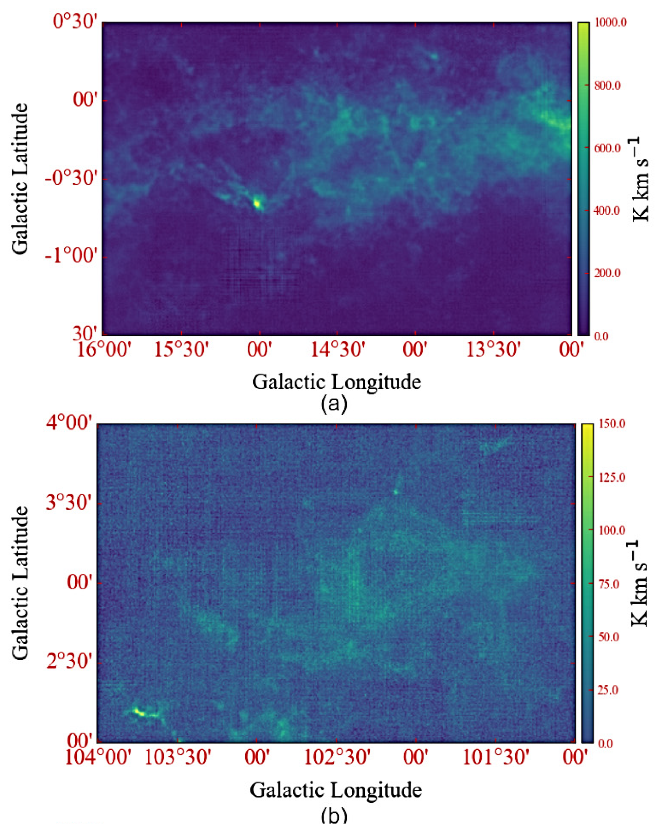
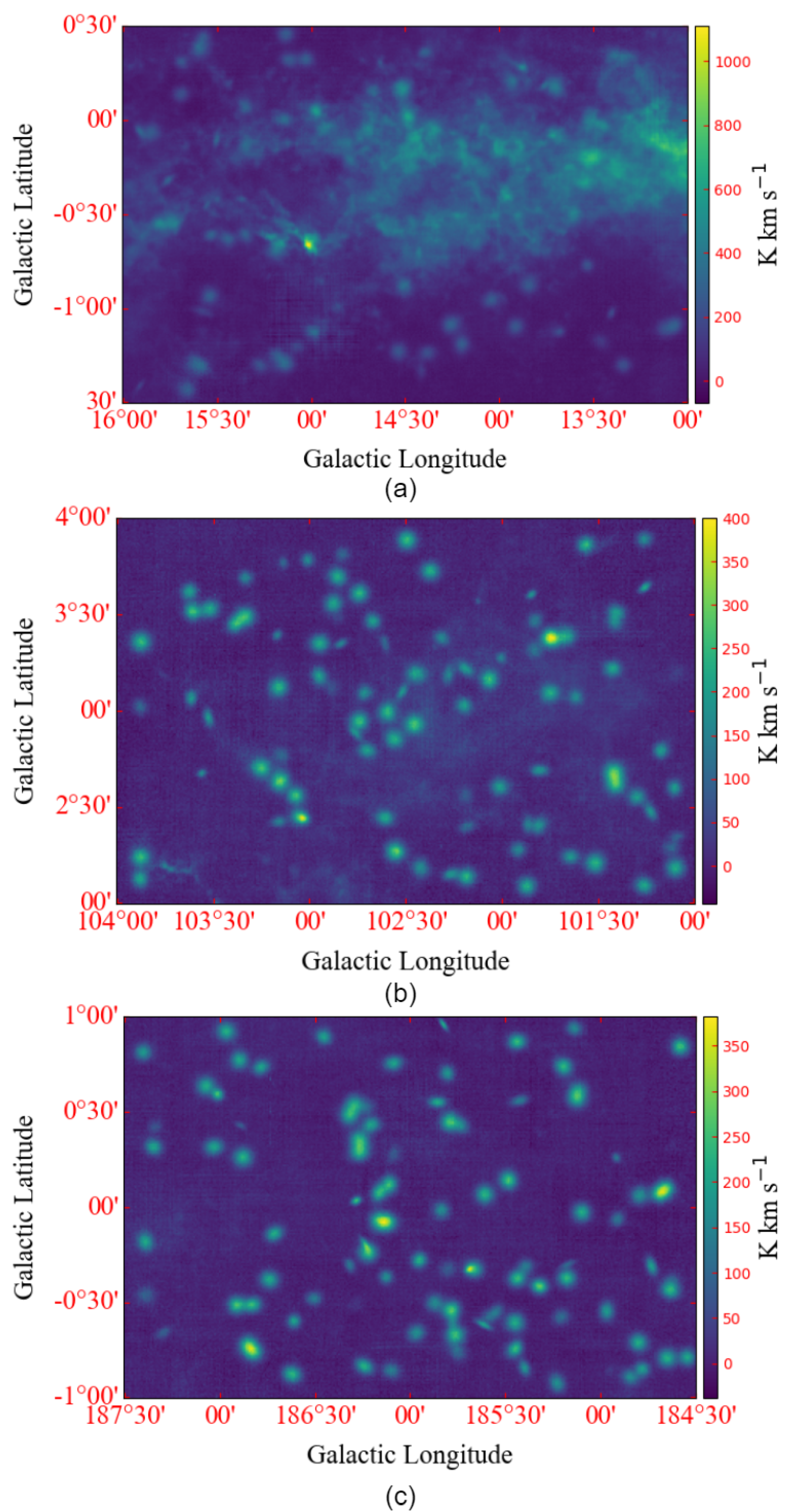
Figure 2.
Velocity—integrated intensity maps for selected background regions. (a) the first Galactic quadrant with and ; the velocity ranges . (b) the second Galactic quadrant with and ; the velocity ranges . (c) the third Galactic quadrant with and ; the velocity ranges .
Figure 2.
Velocity—integrated intensity maps for selected background regions. (a) the first Galactic quadrant with and ; the velocity ranges . (b) the second Galactic quadrant with and ; the velocity ranges . (c) the third Galactic quadrant with and ; the velocity ranges .
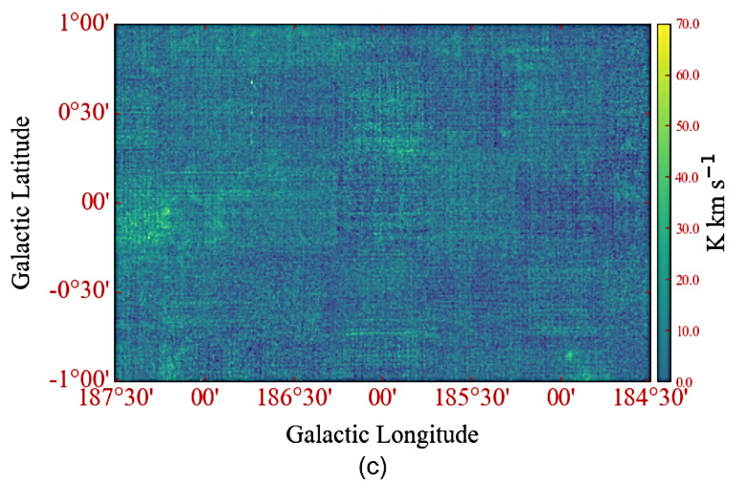
Figure 3.
Velocity—integrated intensity maps of the synthesized data: (a) the first Galactic quadrant synthesized data. (b) the second Galactic quadrant synthesized data. (c) the third Galactic quadrant synthesized data.
Figure 3.
Velocity—integrated intensity maps of the synthesized data: (a) the first Galactic quadrant synthesized data. (b) the second Galactic quadrant synthesized data. (c) the third Galactic quadrant synthesized data.
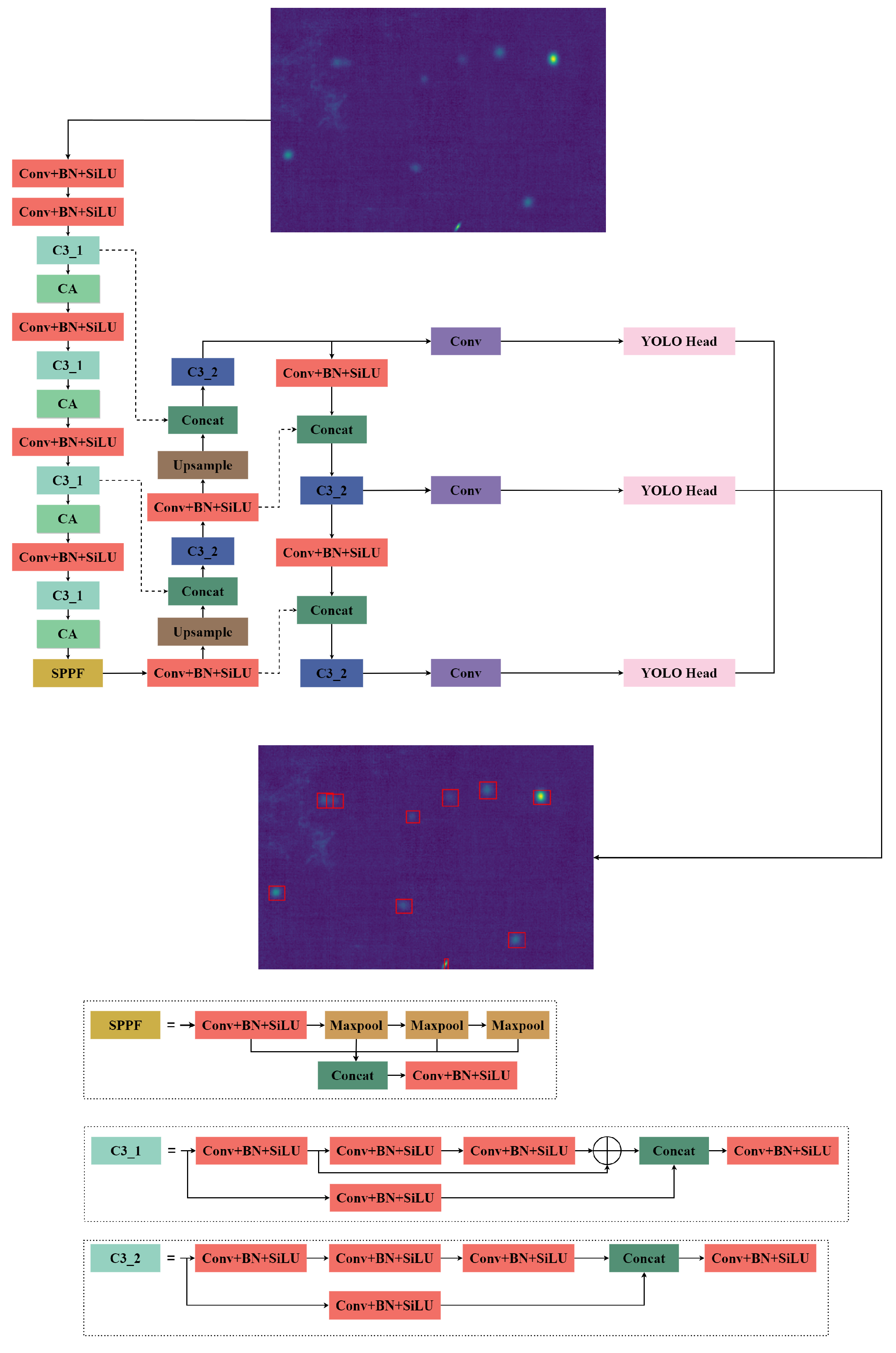
Figure 4.
Architecture of MCD-YOLOv5. MCD-YOLOv5 is mainly composed of three parts: backbone, neck, and YOLO head. The backbone consists of CBS, C3_1, and CA modules. CBS is a composite convolution module, which encapsulates a convolutional layer, a batch normalization layer, and the SiLU activation function. MCD-YOLOv5 contains two types of C3 modules; C3_1 is applied in the backbone and C3_2 is applied in the neck. The C3_1 module and C3_2 module both consist of CBS. In C3_1, the input feature map passes through three branches, while in C3_2, it only passes through two branches. The branches are finally spliced by channel and then output through a CBS module. We add a CA module after each layer of the C3_1. The neck consists of SPPF(Spatial Pyramid Pooling-Fast), and CSP-PAN(CSP-Path Aggregation Network) modules. SPPF is a spatial pyramid pooling module. SPPF encapsulates a CBS module and three maximum pooling layers. Three pooling results with input feature maps are spliced by channel and passed through a CBS module. CSP-PAN is composed of CBS and C3_2, and the feature fusion of different feature layers is realized through upsampling and downsampling, which solves the target multi-scale problem to a certain extent. The main part of the YOLO head is three detectors, that is, using mesh-based anchors to detect objects on feature maps at different scales.
![Universe 09 00480 g004]()
Figure 5.
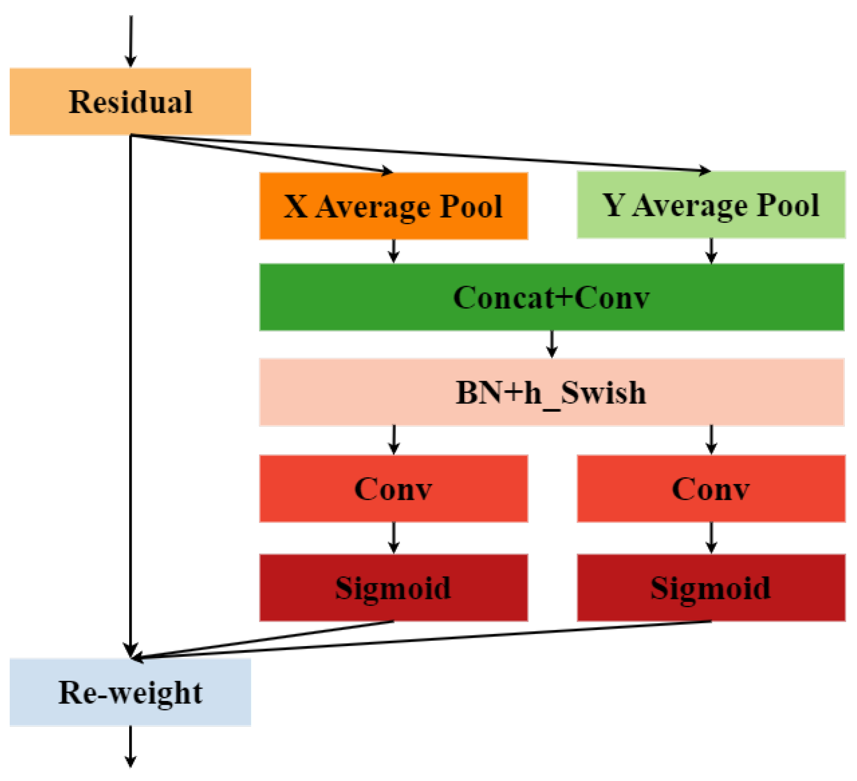
Architecture of Coordinate Attention module. The module is made of two average pooling layers, a convolution layer with concat operation, a batch normalization layer with an h_swish activation function, two convolution layers, and two sigmoid activation functions. The average pooling layers encode each channel of the feature map along the X and Y directions. The resulting feature maps are combined and transformed via the convolution layer with concat operation and the batch normalization layer with an h_swish activation function to create intermediate feature maps. These feature maps are then divided into separate tensors, which are again transformed and expanded by the convolution layer and sigmoid activation function to become the value of the attention weight assignment.
Figure 5.
Architecture of Coordinate Attention module. The module is made of two average pooling layers, a convolution layer with concat operation, a batch normalization layer with an h_swish activation function, two convolution layers, and two sigmoid activation functions. The average pooling layers encode each channel of the feature map along the X and Y directions. The resulting feature maps are combined and transformed via the convolution layer with concat operation and the batch normalization layer with an h_swish activation function to create intermediate feature maps. These feature maps are then divided into separate tensors, which are again transformed and expanded by the convolution layer and sigmoid activation function to become the value of the attention weight assignment.
Figure 6.
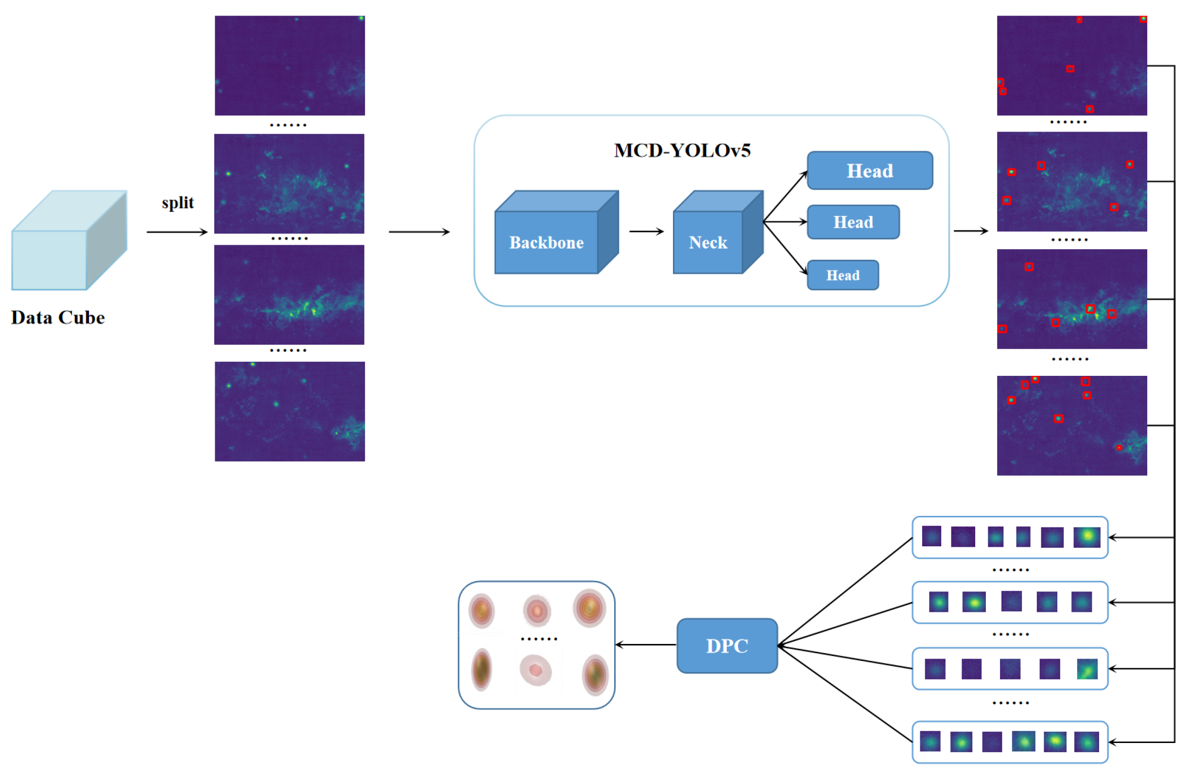
Flowchart of the clump-detection method based on MCD-YOLOv5 joint DPC. The four branches represent any four slices in a given data cube. Each slice achieves 2D detection by MCD-YOLOv5 to obtain the anchor information of the target on the corresponding slice. The rest slices are indicated by ellipses. Heads in different size fonts indicate different scales of detection heads.
Figure 6.
Flowchart of the clump-detection method based on MCD-YOLOv5 joint DPC. The four branches represent any four slices in a given data cube. Each slice achieves 2D detection by MCD-YOLOv5 to obtain the anchor information of the target on the corresponding slice. The rest slices are indicated by ellipses. Heads in different size fonts indicate different scales of detection heads.
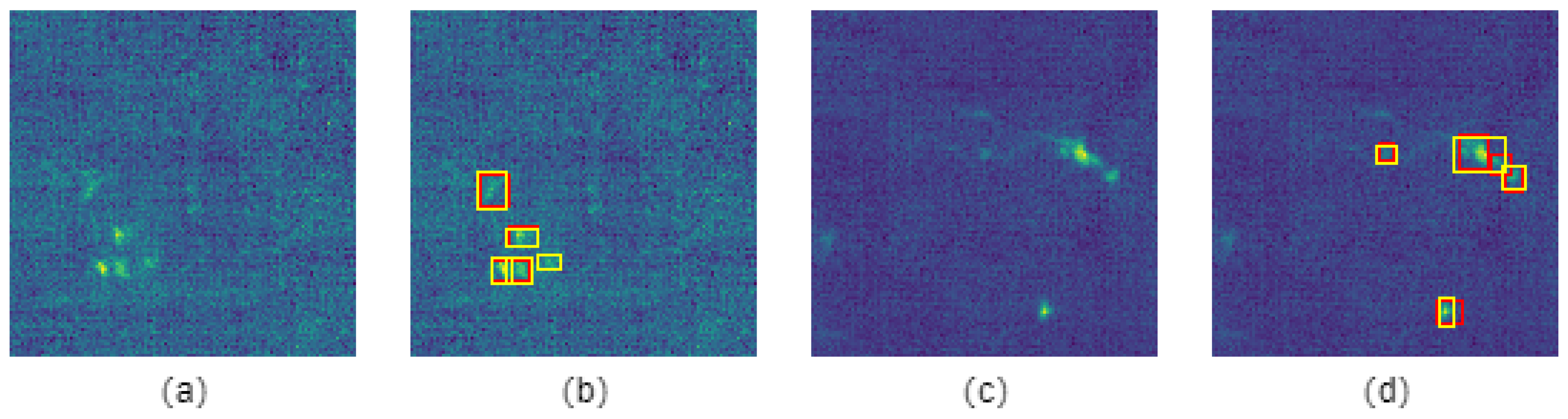
Figure 7.
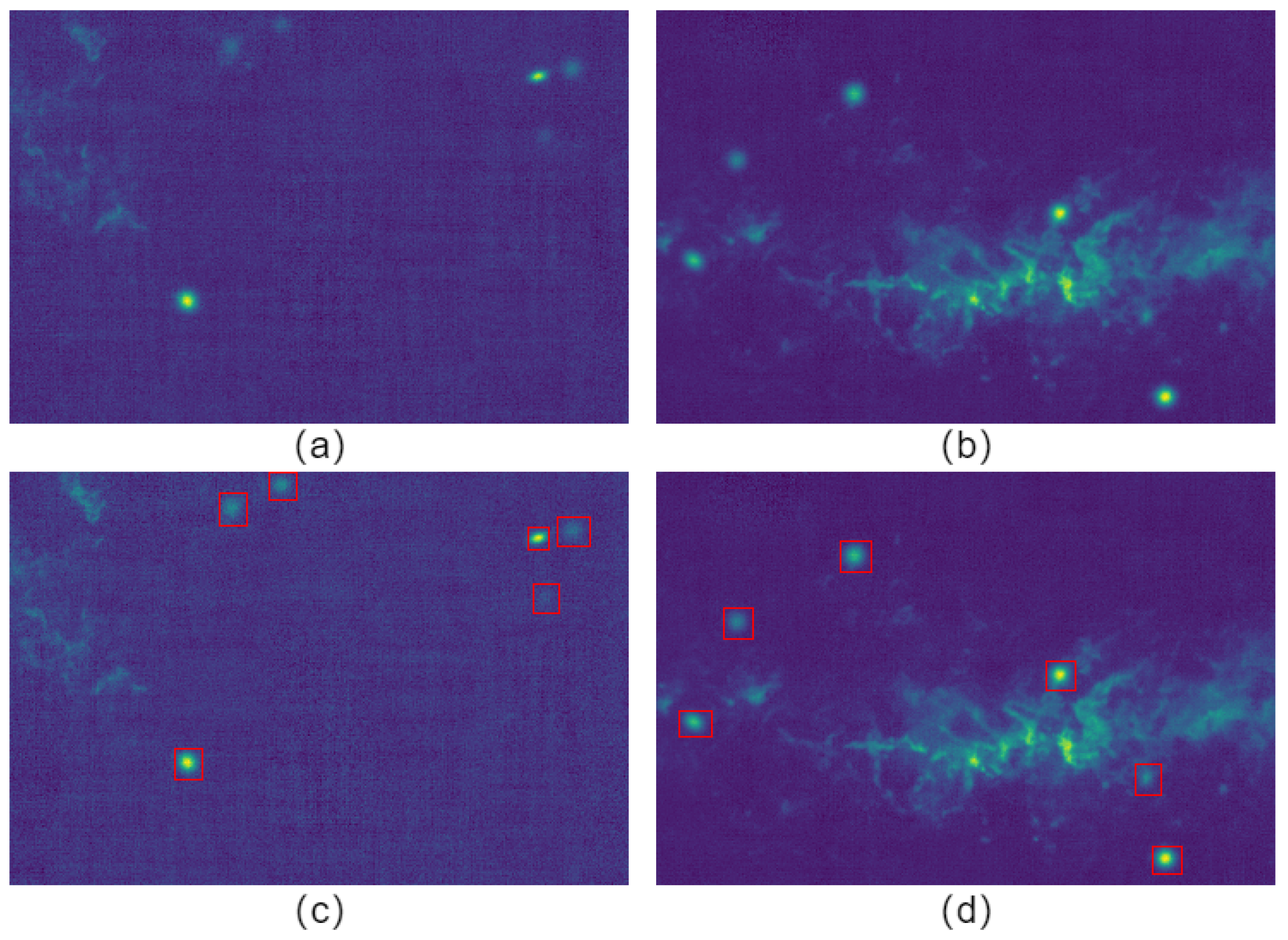
Examples from the MCD-YOLOv5 dataset and the annotation information: (a) synthesized data in the third Galactic quadrant, (b) synthesized data in the first Galactic quadrant, (c) annotation information on (a), and (d) annotation information on (b). The red-labeled boxes represent the clumps.
Figure 7.
Examples from the MCD-YOLOv5 dataset and the annotation information: (a) synthesized data in the third Galactic quadrant, (b) synthesized data in the first Galactic quadrant, (c) annotation information on (a), and (d) annotation information on (b). The red-labeled boxes represent the clumps.
Figure 8.
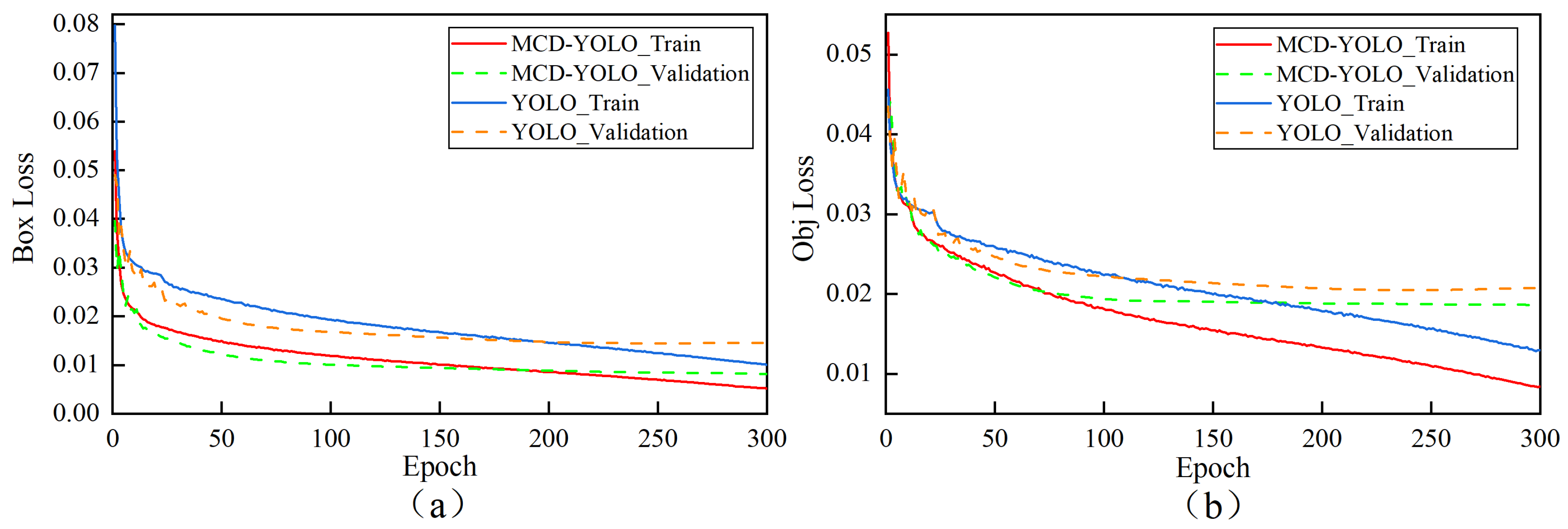
Comparing loss-change curves MCD-YOLOv5 and YOLOv5 training. The clump-detection task has only one category of clump, so the loss contains only localization loss and confidence loss: (a) variation in localization loss (Box Loss) with number of training rounds (epoch), (b) variation in confidence loss (Obj Loss) with number of training rounds (epoch).
Figure 8.
Comparing loss-change curves MCD-YOLOv5 and YOLOv5 training. The clump-detection task has only one category of clump, so the loss contains only localization loss and confidence loss: (a) variation in localization loss (Box Loss) with number of training rounds (epoch), (b) variation in confidence loss (Obj Loss) with number of training rounds (epoch).
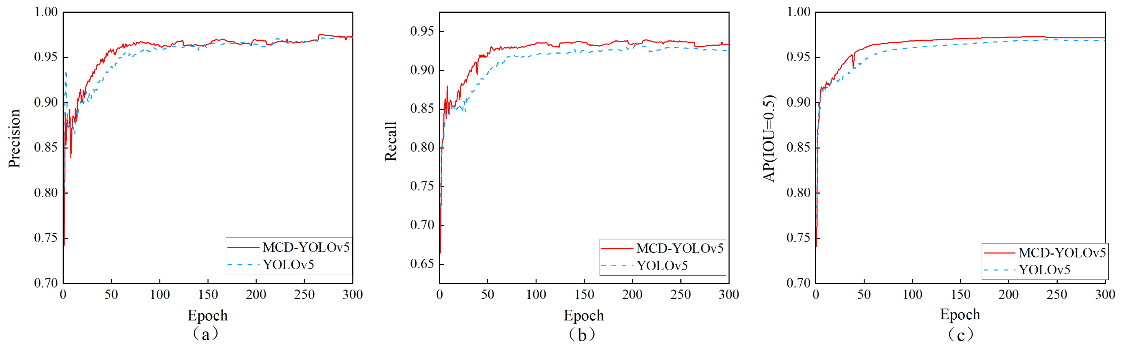
Figure 9.
Variation curves of precision, recall, and AP as a function of the number of training rounds (epoch) for MCD-YOLOv5 and YOLOv5 on the validation set: (a) precision, and (b) recall, and (c) AP.
Figure 9.
Variation curves of precision, recall, and AP as a function of the number of training rounds (epoch) for MCD-YOLOv5 and YOLOv5 on the validation set: (a) precision, and (b) recall, and (c) AP.
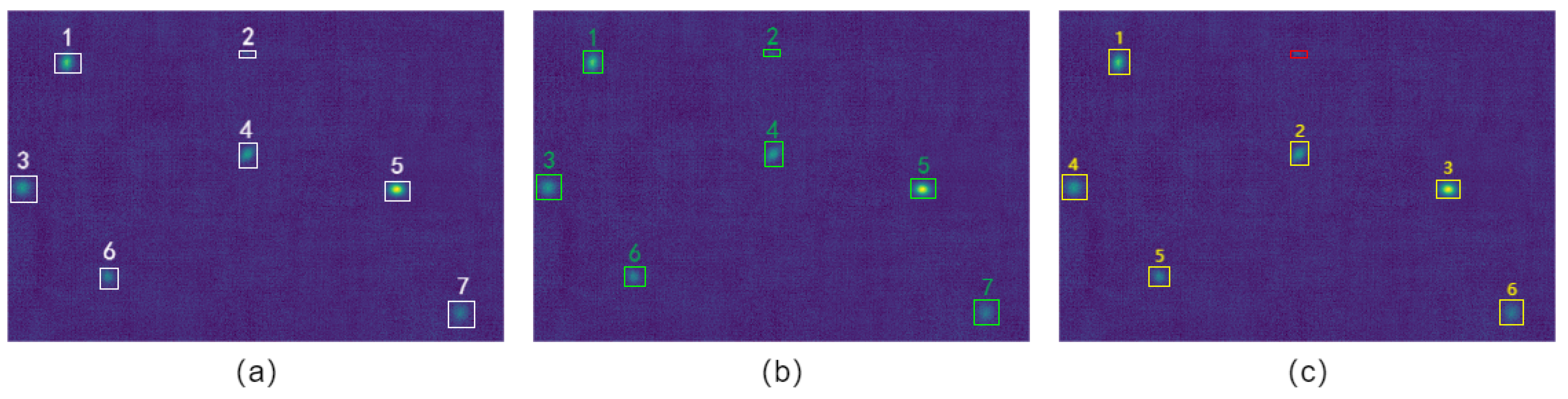
Figure 10.
A typical example of detection results of MCD-YOLOv5 and YOLOv5. (a) Seven simulated clumps in the area. (b) MCD-YOLOv5 detected 7 clumps. (c) YOLOv5 detected 6 clumps. The red rectangular box in (c) represents the missed clump.
Figure 10.
A typical example of detection results of MCD-YOLOv5 and YOLOv5. (a) Seven simulated clumps in the area. (b) MCD-YOLOv5 detected 7 clumps. (c) YOLOv5 detected 6 clumps. The red rectangular box in (c) represents the missed clump.
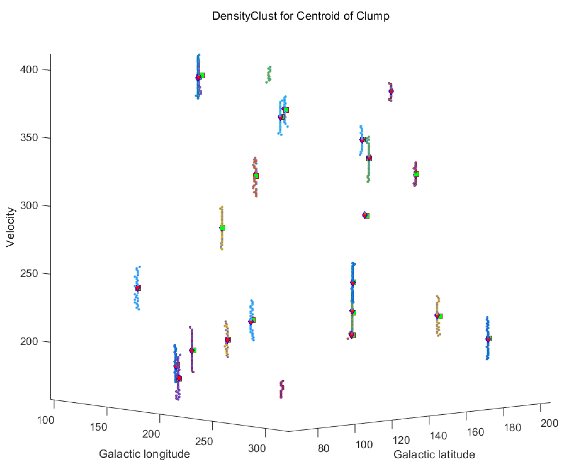
Figure 11.
Display of the DPC results. The differently colored dots represent the center of mass of a clump detected by MCD-YOLOv5, the red rhombus represents a clustering center, and the green square represents the location of the center of mass of a simulated clump.
Figure 11.
Display of the DPC results. The differently colored dots represent the center of mass of a clump detected by MCD-YOLOv5, the red rhombus represents a clustering center, and the green square represents the location of the center of mass of a simulated clump.
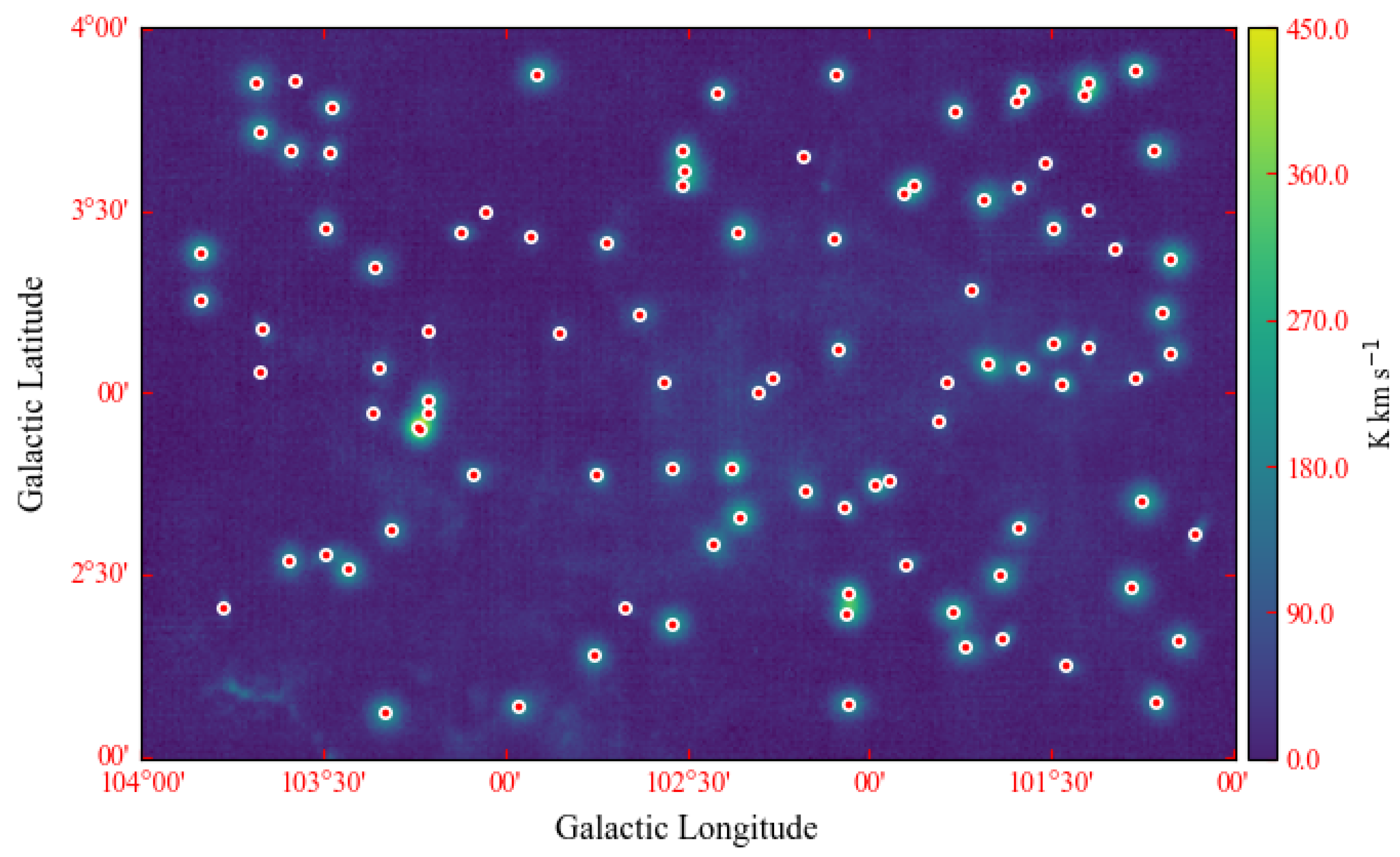
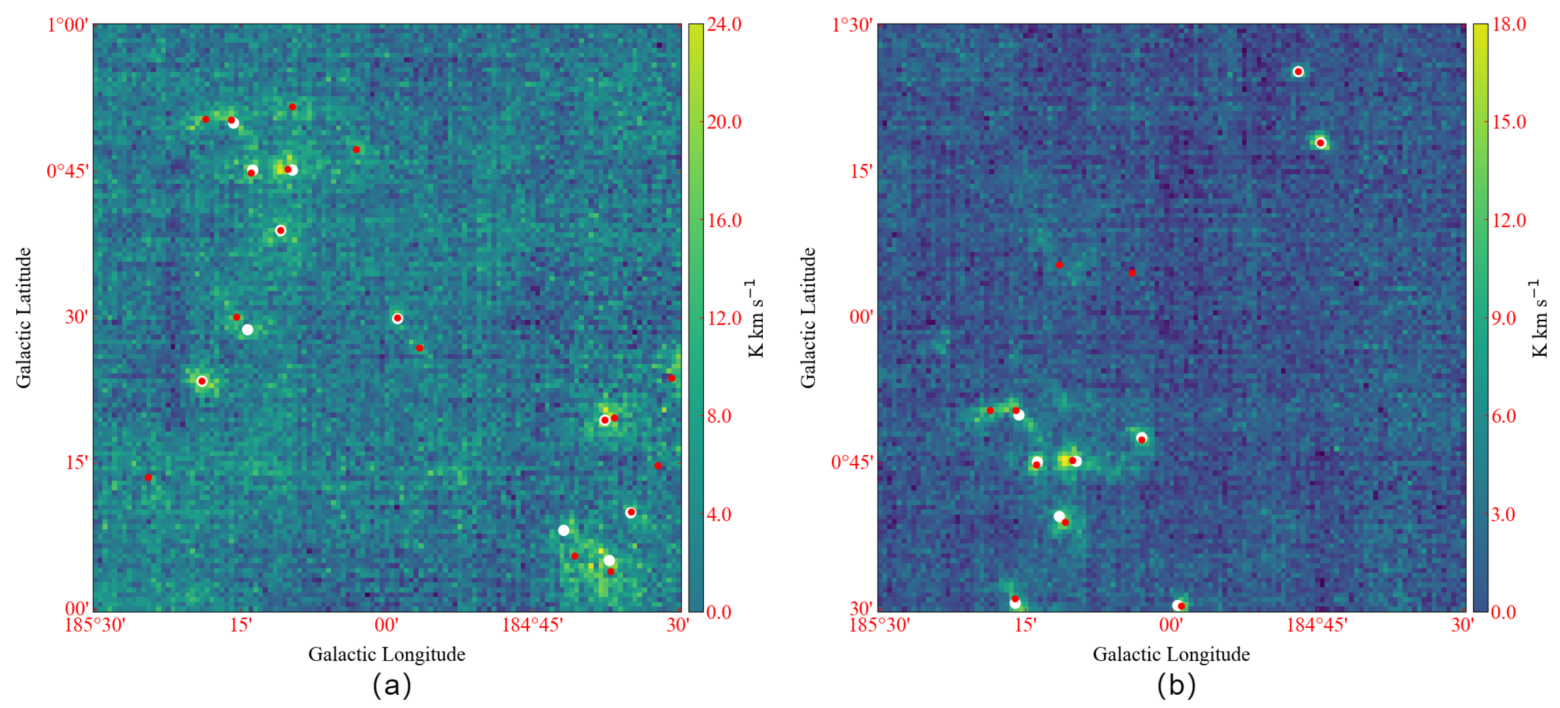
Figure 12.
Velocity—integrated intensity maps of the detection result. The white circles are the center of mass positions of the simulated clumps, and the red dots indicate the center of mass positions of the clumps that are detected and matched with the simulated clumps by MCD-YOLOv5 joint DPC.
Figure 12.
Velocity—integrated intensity maps of the detection result. The white circles are the center of mass positions of the simulated clumps, and the red dots indicate the center of mass positions of the clumps that are detected and matched with the simulated clumps by MCD-YOLOv5 joint DPC.
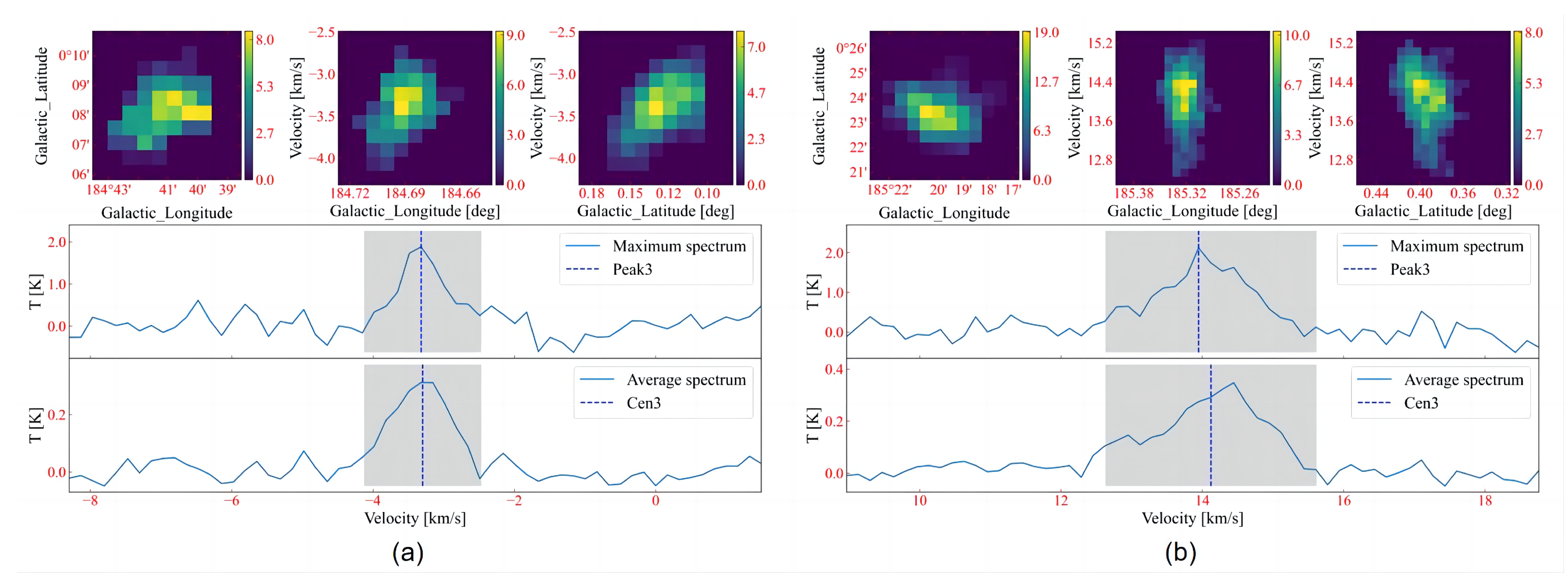
Figure 13.
The information of the simulated clump is shown. (a,b) two examples of the integrated intensity map of the detected clumps of second quadrant synthesized data. The top three subplots offer the l−b, l−v, and b−v maps integration in three directions for a clump, while the middle and bottom of the figure show the peak spectrum and average spectrum of the clump, respectively.
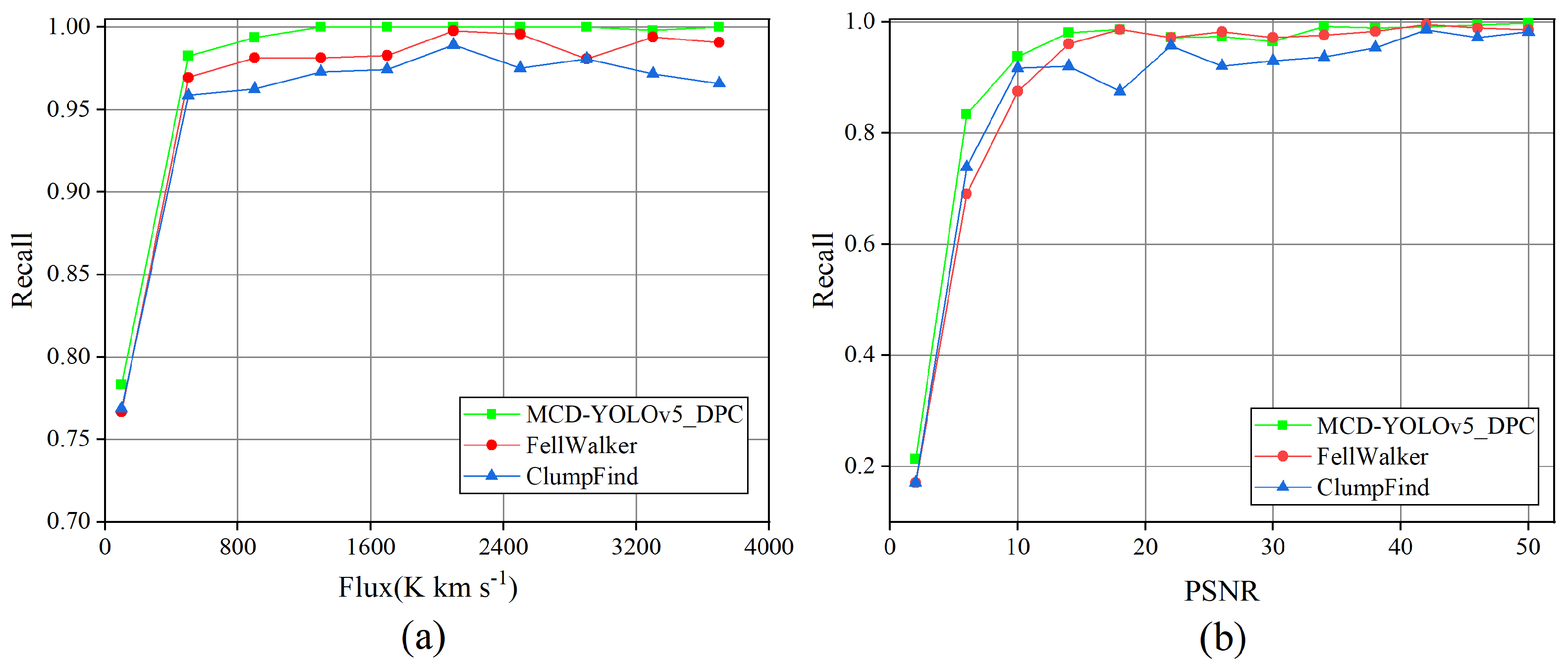
Figure 14.
Variation of recall with flux and PSNR for ClumpFind, FellWalker, and MCD-YOLOv5 joint DPC: (a) Recall variation with flux, and (b) Recall variation with PSNR.
Figure 14.
Variation of recall with flux and PSNR for ClumpFind, FellWalker, and MCD-YOLOv5 joint DPC: (a) Recall variation with flux, and (b) Recall variation with PSNR.
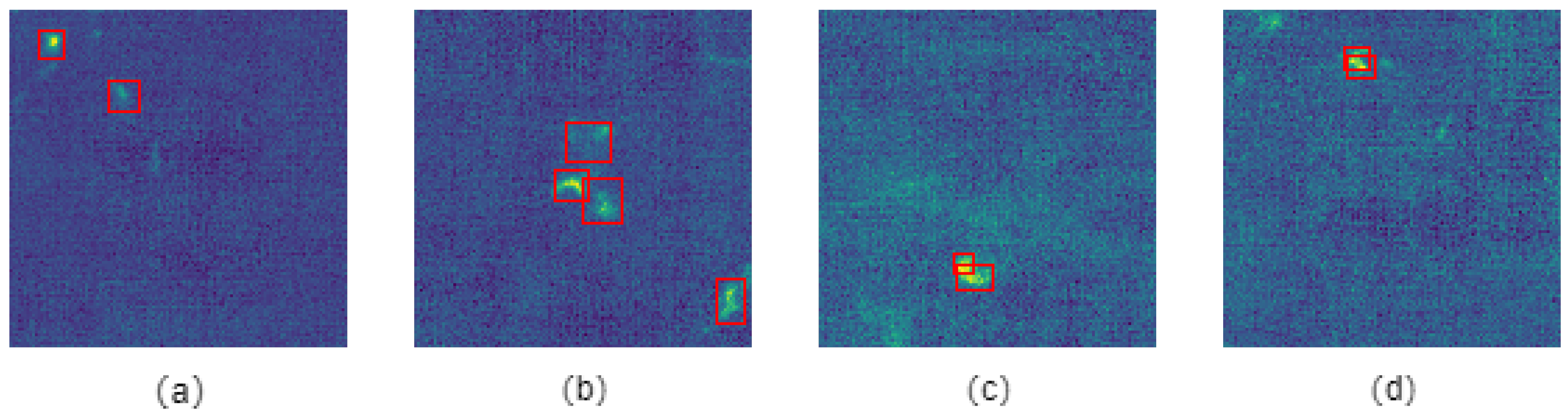
Figure 15.
Examples from the MCD-YOLOv5 dataset and labeling the annotation information on the samples. (a–d) all show the labeling of the observational data slices in the third Galactic quadrant. The red-labeled box is annotation information.
Figure 15.
Examples from the MCD-YOLOv5 dataset and labeling the annotation information on the samples. (a–d) all show the labeling of the observational data slices in the third Galactic quadrant. The red-labeled box is annotation information.
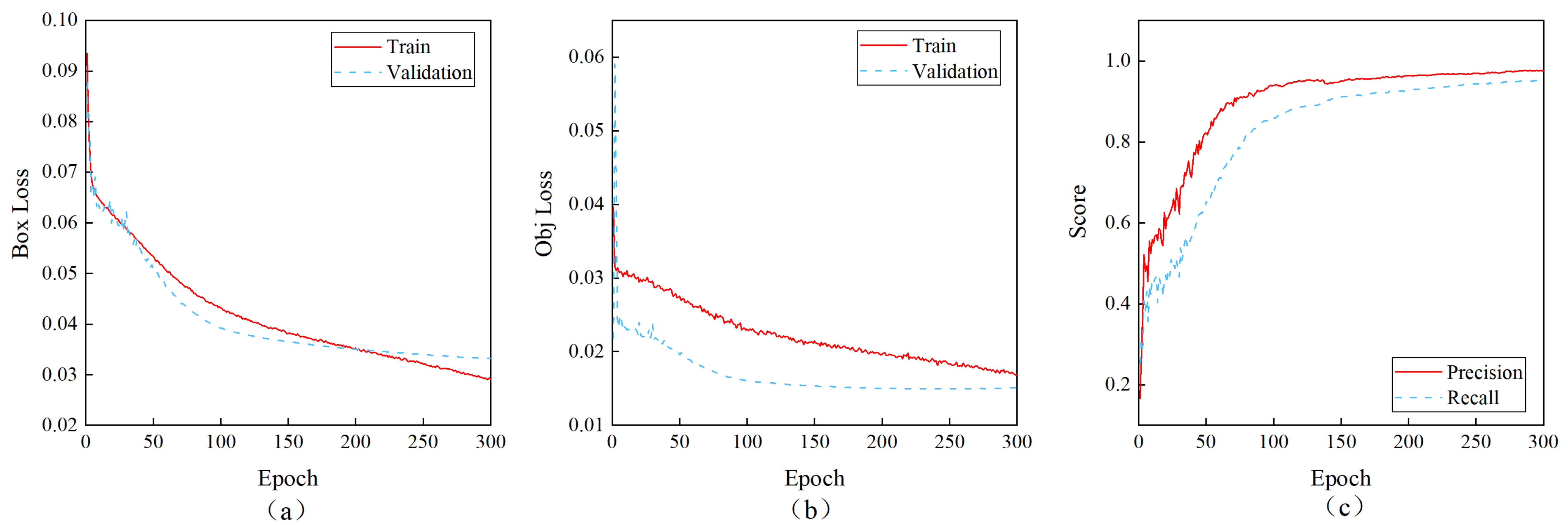
Figure 16.
Variation curves of loss-change, precision, and recall on the validation set of the real dataset during MCD-YOLOv5 training: (a) variation in localization loss, (b) variation in confidence loss, (c) variation in precision and recall.
Figure 16.
Variation curves of loss-change, precision, and recall on the validation set of the real dataset during MCD-YOLOv5 training: (a) variation in localization loss, (b) variation in confidence loss, (c) variation in precision and recall.
Figure 17.
Detection results of MCD-YOLOv5 in observational data. (a,c) the slices generated by intercepting along the velocity channel of the observational data. (b,d) the detection results of MCD-YOLOv5. The red-labeled box is annotation information, the yellow-labeled box is the detection result of MCD-YOLOV5.
Figure 18.
Velocity—integrated intensity maps of detection results. (a,b) velocity—integrated intensity maps of detection results of the two examples. The white circles are the center of mass positions of the clumps detected by MCD-YOLOv5 joint DPC, and the red dots indicate the center of mass positions of the clumps that are detected by FellWalker.
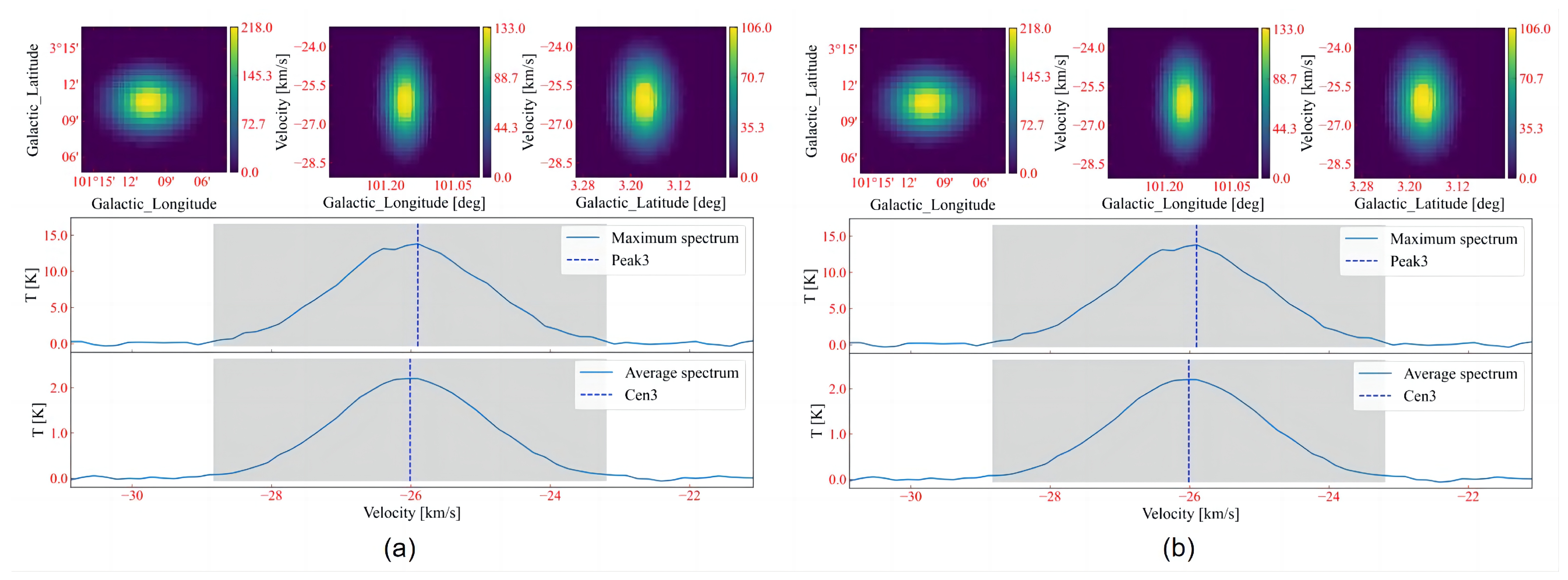
Figure 19.
The information of the clump is shown. (a,b) two examples of the integrated intensity map of the detected clumps of observational data. The top three subplots offer the l−b, l−v, and b−v maps integration in three directions for a clump, while the middle and bottom of the figure show the peak spectrum and average spectrum of the clump, respectively.
Table 1.
Parameters of the 3D Gaussian model.
Table 1.
Parameters of the 3D Gaussian model.
| Parameter Name | Explanation | Range |
|---|
| Peak | Peak intensity of the clump | [0.7, 15] |
| Standard deviation on the Galactic longitude | [1, 4] × 2.3548 |
| Standard deviation on the Galactic latitude | [1, 4] × 2.3548 |
| Standard deviation on the velocity direction | [1, 7] × 2.3548 |
| (, , ) | Position of the center of mass of the clump | Randomization |
| Rotation angle on the Galactic plane | – |
Table 2.
Parameter information table of simulated clumps.
Table 2.
Parameter information table of simulated clumps.
| Parameter Name | Explanation |
|---|
| ID | Clump number |
| Peak1, Peak2, Peak3 | Peak coordinates of clumps |
| Cen1, Cen2, Cen3 | Coordinates of the center of mass of clumps |
| Size1, Size2, Size3 | Axis lengths of clumps in the Galactic plane, and velocity direction |
| Rotation angles of clumps on the Galactic plane |
| Sum | Total flux of clumps |
| Peak | Peak intensity of clumps |
Table 3.
Input and output data for DPC.
Table 3.
Input and output data for DPC.
| Description | Parameters Name | Explanation |
|---|
| | | Galactic longitude coordinates of the center of mass in the region detected by MCD-YOLOv5 |
| | | Galactic latitude coordinates of the center of mass in the region detected by MCD-YOLOv5 |
| Input | | Channels in the velocity direction detected by MCD-YOLOv5 |
| | | Intensity of () in the synthesized data |
| Output | numClust | Number of clustered clumps categories |
Table 4.
Detection results of MCD-YOLOv5 and YOLOv5 on the test set.
Table 4.
Detection results of MCD-YOLOv5 and YOLOv5 on the test set.
| Model | Precision | Recall | AP |
|---|
| MCD-YOLOv5 | 0.969 | 0.935 | 0.972 |
| YOLOv5 | 0.969 | 0.910 | 0.956 |
Table 5.
FellWalker Parameters.
Table 5.
FellWalker Parameters.
| Parameters Name And Default Value |
|---|
| FELLWALKER.ALLOWEDGE = 1 |
| FELLWALKER.CLEANITER = 1 |
| FELLWALKER.FLATSLOPE = 2 × RMS |
| FELLWALKER.FWHMBEAM = 2 |
| FELLWALKER.MAXBAD = 0.05 |
| FELLWALKER.MAXJUMP = 4 |
| FELLWALKER.MINDIP = 1 × RMS |
| FELLWALKER.MINHEIGHT = 3 × RMS |
| FELLWALKER.MINPIX = 27 |
| FELLWALKER.NOISE = 2 × RMS |
| FELLWALKER.VELORES = 2 |
Table 6.
ClumpFind parameters.
Table 6.
ClumpFind parameters.
| Parameters Name And Default Value |
|---|
| CLUMPFIND.ALLOWEDGE = 1 |
| CLUMPFIND.DELTAT = 2 × RMS |
| CLUMPFIND.FWHMBEAM = 2 |
| CLUMPFIND.IDLAIG = 1 |
| CLUMPFIND.MAXBAD = 0.05 |
| CLUMPFIND.MINPIX = 27 |
| CLUMPFIND.NAXIS = 3 |
| CLUMPFIND.NOISE = 2 × RMS |
| CLUMPFIND.TLOW = 3 × RMS |
| CLUMPFIND.VELORES = 2 |
Table 7.
MCD-YOLOv5 joint DPC parameters. minRho represents the minimum peak intensity of the clump, i.e., the point corresponding to this intensity can be used as the cluster center during the DPC clustering process. minRho can be set according to the intensity characteristics of the clumps in different regions. minDelta represents the minimum pixel distance to distinguish between two clumps. minDelta can be set according to the sparseness of the clump distribution.
| Parameters Name | Explanation | Default Value |
|---|
| minRho | The minimum intensity of clump | [2, 5] × RMS |
| minDelta | The minimum pixel distance to distinguish between two clumps | 4 |
Table 8.
Detection results of MCD-YOLOv5 joint DPC, FellWalker, and ClumpFind.
Table 8.
Detection results of MCD-YOLOv5 joint DPC, FellWalker, and ClumpFind.
| Method | Matched Clumps | Recall |
|---|
| MCD-YOLOv5 joint DPC | 9841 | 98.41% |
| FellWalker | 9770 | |
| ClumpFind | 9631 | |

 ,
, 


