
Closed Timelike Curves Induced by a Buchdahl-Inspired Vacuum Spacetime in


Abstract
:1. Introduction
2. The Special Buchdahl-Inspired Metric: Brief Review
3. The –Kruskal–Szekeres Coordinates
- The tortoise coordinate for the special Buchdahl-inspired metric (9) is defined by virtue ofThis equation is soluble, yielding the tortoise coordinate in terms of a Gaussian hypergeometric functionwhich is represented in Figure 1. The integration constant required for Equation (11) has been chosen such that when .
- The advanced and retarded Eddington–Finkelstein coordinates are defined asrespectively.
- For the Kruskal–Szekeres (KS) coordinates, it is necessary to separate the two ranges, versus .
- -
- For , we define
- -
- For , we define
4. The -Kruskal–Szekeres Diagram
- The –KS diagram is conformally Minkowski. The null geodesics are .
- Per Equations (20) and (21), a constant–r contour corresponds to a hyperbola, while a constant–t contour corresponds to a straight line running through the origin of the plane. The coordinate origin amounts to , since .
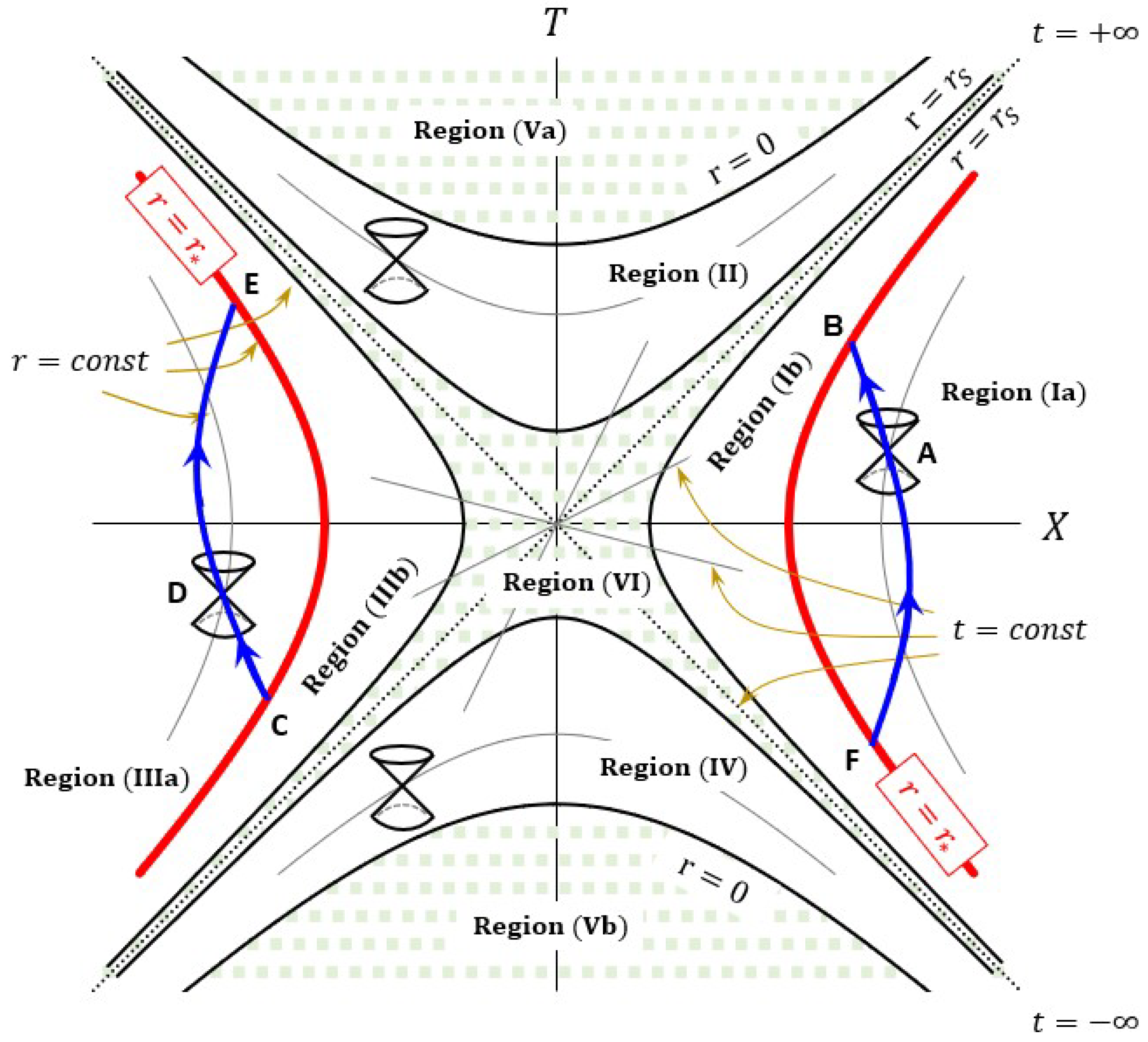
- The boundary corresponds to two distinct hyperbolae, given bySince each hyperbola has two separate branches on its own, Figure 2 shows four branches representing in total. For (i.e., ), the hyperbolic branches (22) degenerate into two straight lines, , as is expected for the Schwarzschild metric. In the limit of , Region (VI), which sandwiches within the four hyperbolic branches, shrinks and disappears.
- Region (I) refers to (the “exterior”); Region (II) refers to .
- Regions (III) and (IV) are double copies of Regions (I) and (II) respectively, by flipping the sign of the KS coordinates, viz. . Regions (Va) and (Vb) are unphysical, viz. .
- Region (VI) generally contains curvature singularities, with the Kretschmann scalar generally diverging on the hyperbolic branches given in (22). The “gulf” represented by Region (VI) is a new feature of the asymptotically flat Buchdahl-inspired spacetimes. The Kretschmann invariant is reproduced in Appendix A.
Areal Radius
5. Naked Singularity: Case
6. Wormhole: Case
- The traveller enters the right mouth of the wormhole at point B after a finite amount of proper time. From the perspective of an observer at rest in Region (Ia), it also takes a finite amount of time for the traveller to reach point B.
- Subsequently, the traveller emerges from the left mouth of the wormhole at point C (note: point B and point C are identical!). They then ascend the potential well (viz. increasing r), moving toward point D. It is important to note that, relative to the observer in Region (Ia), the traveller appears to move backward in time, as the t coordinate decreases from point C to point D.
- If the traveller chooses to fall back into the left mouth, they will re-enter it at point E. They will then re-emerge at the right mouth at point F (which is identical to point E!). Notably, upon re-emergence, they are once again moving forward in time.
- At this stage, the traveller can choose to proceed to point A, thereby completing a closed timelike loop.
7. Discussions and Summary
- It is worth highlighting that the CTC we have described does not require having one wormhole mouth move at high speed or be located near a supermassive object to accumulate time dilation, as popularized in [2,6,19]. To the best of our knowledge, the CTC presented herewith has not been documented in the existing literature.
- Our association of a pair of antipodal points (such as B and C) with a single spacetime event was inspired by a similar construction proposed by Popławski. In [23], he revisited the Einstein–Rosen (ER) bridge and identified two antipodal points on the horizon with a single spacetime event. The ER bridge was interpreted as a “Schwarzschild wormhole” connecting the two exterior sheets joined at the horizon. However, the ER bridge encounters various issues related to traversability, stability, and a problematic thin-shell mass distribution at the horizon. (It is also worth noting that Popławski did not suggest the possibility of CTCs in his work.)
- The Morris–Thorne–Buchdahl wormhole, developed in [22] and briefly summarized in this paper, appears to avoid the issues faced in Popławski’s work. Setting aside the physical questions regarding causality violations and time-travel-related paradoxes, our construction of a CTC appears to be mathematically consistent.
- Central to our approach is the identification of any given pair of antipodal points on the loci of minimum areal radius, denoted as , with a single spacetime event. This identification becomes evident through Equations (20) and (21), as well as in the KS diagrams employed for the Schwarzschild metric (used in Popławski’s work) and our special Buchdahl-inspired metric in Figure 6.
- Embedding diagrams, such as the one in Figure 5, depict a “snapshot” of the wormhole at a fixed timeslice, without illustrating the evolution of timelike trajectories. As such, the use of embedding diagrams may obscure the identification of spacetime events on the throat, a procedure we carried out in this paper. In this regard, the decisive advantage of KS diagrams is their ability to reveal the full causal structure of spacetime, making this identification transparent.
- Let us draw a comparison between our CTC and the Deutsch-Politzer (DP) time machine.
- In [27,28], a DP space is created from a two-dimensional Minkowski spacetime by making two finite-size “space-like” cuts and gluing the edges of the cuts, effectively forming a “handle” which connects two space-like regions and creates a time machine. The essence of a DP time machine is that the spacetime topology is altered [Note that the DP space has singularities; to exorcise them, in [29,30] Krasnikov performed a conformal transformation to send the singular points away to infinity].
- Our CTC construction shares both analogies and differences with the DP time machine. The –KS diagram of the Buchdahl-inspired vacuum (Figure 6) is a two-dimensional Minkowski spacetime (modulo a Weyl transformation). For , the hyperbolic branches of are glued to form a portal between the two time-reversed sheets, viz. Regions (Ia) and (IIIa). In this regard, akin to the DP space, our construction is a concrete realization of a time machine induced by an alteration in the topology of spacetime.
- Unlike the deliberate surgery employed in the DP space, the alteration of the topology in the Buchdahl-inspired vacuum occurs naturally, driven by the fourth-derivative dynamics of pure gravity. (Also, similar to Krasnikov’s work [29,30], Regions (Ia) and (IIIa) in our –KS diagram are devoid of (physical) singularities.) A comprehensive discussion of their commonalities and differences exceeds the scope of this paper.
- Our CTC construction is not confined solely to the MTB wormholes of pure gravity. It is also applicable to two-way traversable wormholes in Brans–Dicke (BD) gravity, which share a similar Kruskal–Szekeres diagram, as demonstrated in Ref. [24] by one of the authors.
- More generally, the Brans wormhole, first established by Agnese and La Camera for BD gravity in [31,32], encompasses the MTB wormhole in gravity [24]. It is known that a static vacuum solution of any gravity cannot host a twice asymptotically flat wormhole [33]. However, a cut-and-paste procedure can be employed to generate such a wormhole, a technique that underlies the creation of the Brans wormhole [31,32,34,35].
- The MTB wormhole satisfies the four “traversability-in-principle” criteria laid out by Morris and Thorne [1]. To be considered “usable”, the tidal forces should remain finite. We have computed the tidal forces in Appendix B. Our findings indicate that despite jumps in higher derivatives across the throat in the metric components, the tidal forces remain finite throughout the two asymptotically flat spacetime sheets.
Author Contributions
Funding
Institutional Review Board Statement
Informed Consent Statement
Data Availability Statement
Acknowledgments
Conflicts of Interest
Appendix A. Kretschmann Scalar
- At : , , , , giving in agreement with the standard result fort the Schwarzschild metric.
- At : , , , , giving .
- For and , as , K generally diverges at and .
Appendix B. Tidal Forces in MTB and Brans Wormholes
References
- Morris, M.S.; Thorne, K.S. Wormholes in spacetime and their for interstellar travel: A tool for teaching general relativity. Am. J. Phys. 1988, 56, 395. [Google Scholar] [CrossRef]
- Visser, M. Lorentzian Wormholes: From Einstein to Hawking; Springer: New York, NY, USA, 1996; ISBN 9781563966538. [Google Scholar]
- Alcubierre, M.; Lobo, F.S.N. Wormholes, Warp Drives and Energy Conditions. Fundam. Theor. Phys. 2017, 189, 257–279. [Google Scholar]
- Lobo, F.S.N.; Oliveira, M.A. Wormhole geometries in f(R) modified theories of gravity. Phys. Rev. D 2009, 80, 104012. [Google Scholar] [CrossRef]
- Harko, T.; Lobo, F.S.N.; Mak, M.K.; Sushkov, S.V. Modified-gravity wormholes without exotic matter. Phys. Rev. D 2013, 87, 067504. [Google Scholar] [CrossRef]
- Morris, M.S.; Thorne, K.S.; Yurtsever, U. Wormholes, Time Machines, and the Weak Energy Condition. Phys. Rev. Lett. 1988, 61, 1446. [Google Scholar] [CrossRef] [PubMed]
- Novikov, I.D. An analysis of the operation of a time machine. Sov. Phys. JETP 1989, 68, 3. [Google Scholar]
- Frolov, V.P.; Novikov, I.D. Physical effects in wormholes and time machines. Phys. Rev. D 1990, 42, 1057. [Google Scholar] [CrossRef] [PubMed]
- Friedman, J.L.; Morris, M.S.; Novikov, I.D.; Echeverria, F.; Klinkhammer, G.; Thorne, K.S.; Yurtsever, U. Cauchy problem in spacetimes with closed timelike curves. Phys. Rev. D 1990, 42, 1915. [Google Scholar] [CrossRef]
- Gödel, K. An Example of a New Type of Cosmological Solution of Einstein’s Field Equations of Gravitation. Rev. Mod. Phys. 1949, 21, 447. [Google Scholar] [CrossRef]
- Pfarr, J. Time travel in Gödel’s space. Gen. Rel. Grav. 1981, 13, 1073. [Google Scholar] [CrossRef]
- Tipler, F.J. Causality violation in asymptotically flat space-times. Phys. Rev. Lett. 1976, 37, 879. [Google Scholar] [CrossRef]
- de Felice, F.; Calvani, M. Time machine and geodesic motion in Kerr metric. Gen. Rel. Grav. 1978, 9, 155. [Google Scholar]
- Gott, J.R. Closed Timelike Curves Produced by Pairs of Moving Cosmic Strings: Exact Solutions. Phys. Rev. Lett. 1991, 66, 1126. [Google Scholar] [CrossRef] [PubMed]
- Ori, A. Must time machine construction violate the weak energy condition? Phys. Rev. Lett. 1993, 71, 2517. [Google Scholar] [CrossRef] [PubMed]
- Ori, A. A class of time-machine solutions with a compact vacuum core. Phys. Rev. Lett. 2005, 95, 021101. [Google Scholar] [CrossRef]
- Alcubierre, M. The warp drive: Hyperfast travel within general relativity. Class. Quant. Grav. 1994, 11, L73. [Google Scholar] [CrossRef]
- Everett, A.E. Warp drive and causality. Phys. Rev. D 1996, 53, 7365. [Google Scholar] [CrossRef] [PubMed]
- Lobo, F.S.N. Closed timelike curves and causality violation. arXiv 2010, arXiv:1008.1127. [Google Scholar]
- Nguyen, H.K. Beyond Schwarzschild-de Sitter spacetimes: II. An exact non-Schwarzschild metric in pure R2 gravity and new anomalous properties of R2 spacetimes. Phys. Rev. D 2023, 107, 104008. [Google Scholar] [CrossRef]
- Buchdahl, H.A. On the Gravitational Field Equations Arising from the Square of the Gaussian Curvature. Nuovo Cimento 1962, 23, 141. [Google Scholar] [CrossRef]
- Nguyen, H.K.; Azreg-Aïnou, M. Traversable Morris-Thorne-Buchdahl wormholes in quadratic gravity. Eur. Phys. J. C 2023, 83, 626. [Google Scholar] [CrossRef]
- Popławski, N.J. Radial motion motion into an Einstein–Rosen bridge. Phys. Lett. B 2010, 687, 110. [Google Scholar] [CrossRef]
- Nguyen, H.K.; Azreg-Aïnou, M. Revisiting Weak Energy Condition and wormholes in Brans-Dicke gravity. arXiv 2023, arXiv:2305.15450. [Google Scholar]
- Nguyen, H.K. Beyond Schwarzschild-de Sitter spacetimes: A new exhaustive class of metrics inspired by Buchdahl for pure R2 gravity in a compact form. Phys. Rev. D 2022, 106, 104004. [Google Scholar] [CrossRef]
- Nguyen, H.K. Buchdahl-inspired spacetimes and wormholes: Unearthing Hans Buchdahl’s other ‘hidden’ treasure trove. Int. J. Mod. Phys. D 2023, 2342007. [Google Scholar] [CrossRef]
- Deutsch, D. Quantum mechanics near closed timelike lines. Phys. Rev. D 1991, 44, 3197. [Google Scholar] [CrossRef]
- Politzer, H.D. Simple quantum systems in spacetimes with closed timelike curves. Phys. Rev. D 1992, 46, 4470. [Google Scholar] [CrossRef]
- Krasnikov, S.V. A singularity-free WEC-respecting time machine. Class. Quant. Grav. 1998, 15, 997. [Google Scholar] [CrossRef]
- Krasnikov, S.V. Topology Change without any Pathology. Gen. Rel. Gravit. 1995, 27, 529. [Google Scholar] [CrossRef]
- Agnese, A.G.; La Camera, M. Wormholes in the Brans-Dicke theory of gravitation. Phys. Rev. D 1995, 51, 2011. [Google Scholar] [CrossRef]
- Agnese, A.G.; La Camera, M. Schwarzschild metrics, quasi-universes and wormholes. In Frontiers of Fundamental Physics 4; Sidharth, B.G., Altaisky, M.V., Eds.; Kluwer Academic/Plenum Publishers: New York, NY, USA, 2001; p. 197. [Google Scholar]
- Bronnikov, K.A.; Skvortsova, M.V.; Starobinsky, A.A. Notes on wormhole existence in scalar-tensor and F(R) gravity. Grav. Cosmol. 2010, 16, 216. [Google Scholar] [CrossRef]
- Nandi, K.K.; Islam, A. Brans wormhole. Phys. Rev. D 1997, 55, 2497. [Google Scholar] [CrossRef]
- Vanzo, L.; Zerbini, S.; Faraoni, V. Campanelli-Lousto and veiled spacetimes. Phys. Rev. D 2012, 86, 084031. [Google Scholar] [CrossRef]
- Earman, J. Bangs, Crunches, Whimpers, and Shrieks: Singularities and Acausalities in Relativistic Spacetimes; Oxford University Press: Oxford, UK, 1995. [Google Scholar]
- Echeverria, F.G.; Klinkhammer, G.; Thorne, K.S. Billiard Balls in Wormhole Spacetimes with Closed Timelike Curves: Classical Theory. Phys. Rev. D 1991, 44, 1077. [Google Scholar] [CrossRef]
- Novikov, I.D. Time machine and self-consistent evolution in problems with self-interaction. Phys. Rev. D 1992, 45, 1989. [Google Scholar] [CrossRef] [PubMed]
- Hawking, S.W. Chronology protection conjecture. Phys. Rev. D 1992, 46, 603. [Google Scholar] [CrossRef]
- Bronnikov, K.A.; Constantinidis, C.P.; Evangelista, R.L.; Fabris, J.C. Cold black holes in scalar-tensor theories. arXiv 1997, arXiv:gr-qc/9710092. [Google Scholar]
- Visser, M.; Hochberg, D. Generic wormhole throats. Ann. Isr. Phys. 1997, 13, 249. [Google Scholar]


Disclaimer/Publisher’s Note: The statements, opinions and data contained in all publications are solely those of the individual author(s) and contributor(s) and not of MDPI and/or the editor(s). MDPI and/or the editor(s) disclaim responsibility for any injury to people or property resulting from any ideas, methods, instructions or products referred to in the content. |
© 2023 by the authors. Licensee MDPI, Basel, Switzerland. This article is an open access article distributed under the terms and conditions of the Creative Commons Attribution (CC BY) license (https://creativecommons.org/licenses/by/4.0/).
Share and Cite
Nguyen, H.K.; Lobo, F.S.N.
Closed Timelike Curves Induced by a Buchdahl-Inspired Vacuum Spacetime in
Nguyen HK, Lobo FSN.
Closed Timelike Curves Induced by a Buchdahl-Inspired Vacuum Spacetime in
Nguyen, Hoang Ky, and Francisco S. N. Lobo.
2023. "Closed Timelike Curves Induced by a Buchdahl-Inspired Vacuum Spacetime in