
Weak Coupling Regime in Dilatonic
 and
and
Abstract
:1. Introduction
2. Gravitational Field Equations of Gravity
3. Stringy Cosmology
4. Cosmology in Dilatonic Gravity
4.1. Model
4.2. Numerics
5. Results
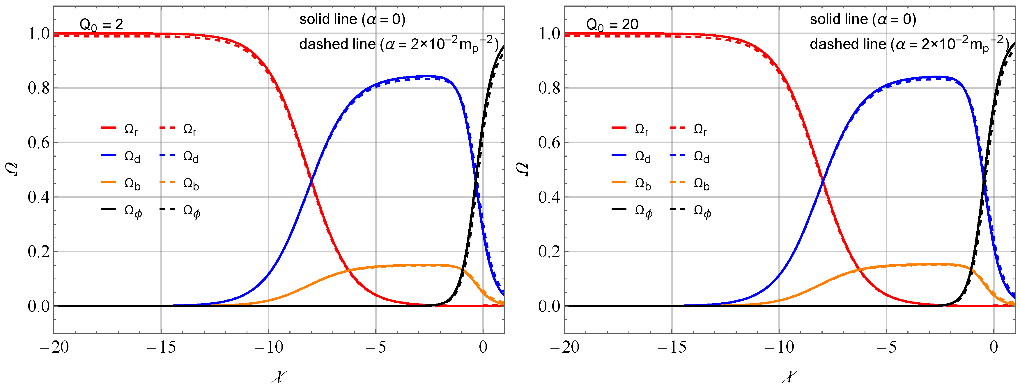
5.1. The Density Parameters , , and
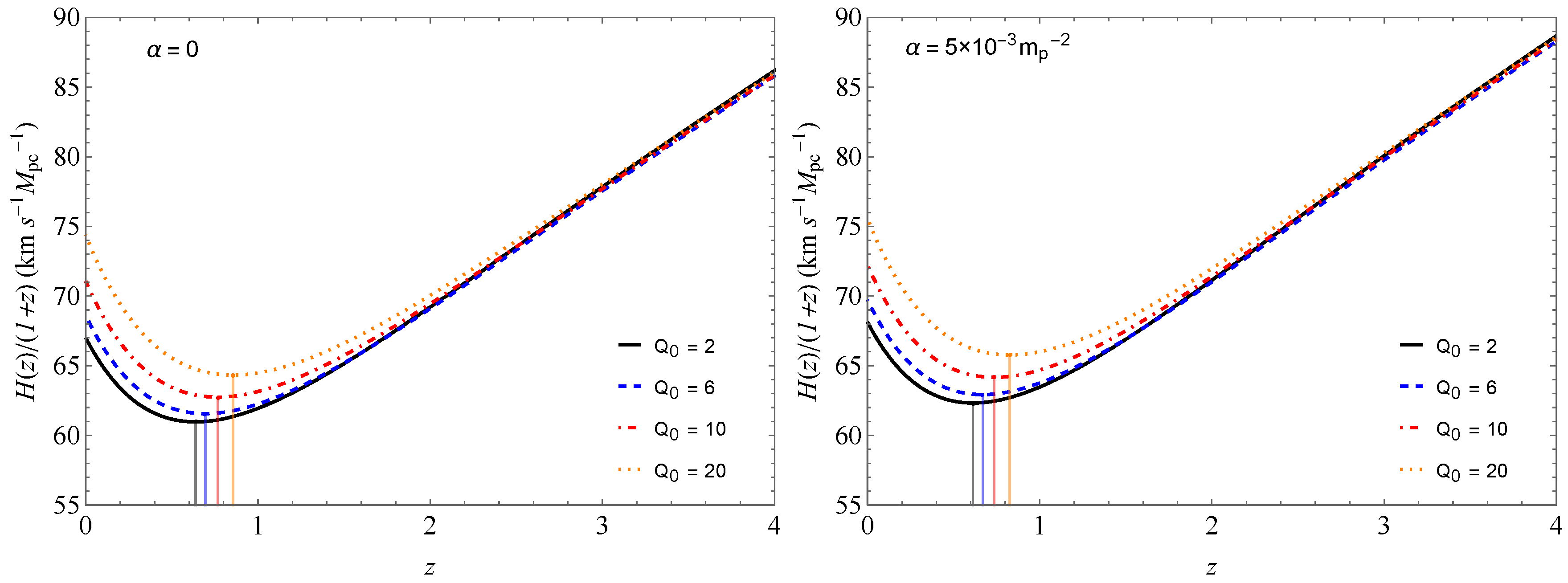
5.2. The Hubble Parameter
5.3. The Dilaton Field
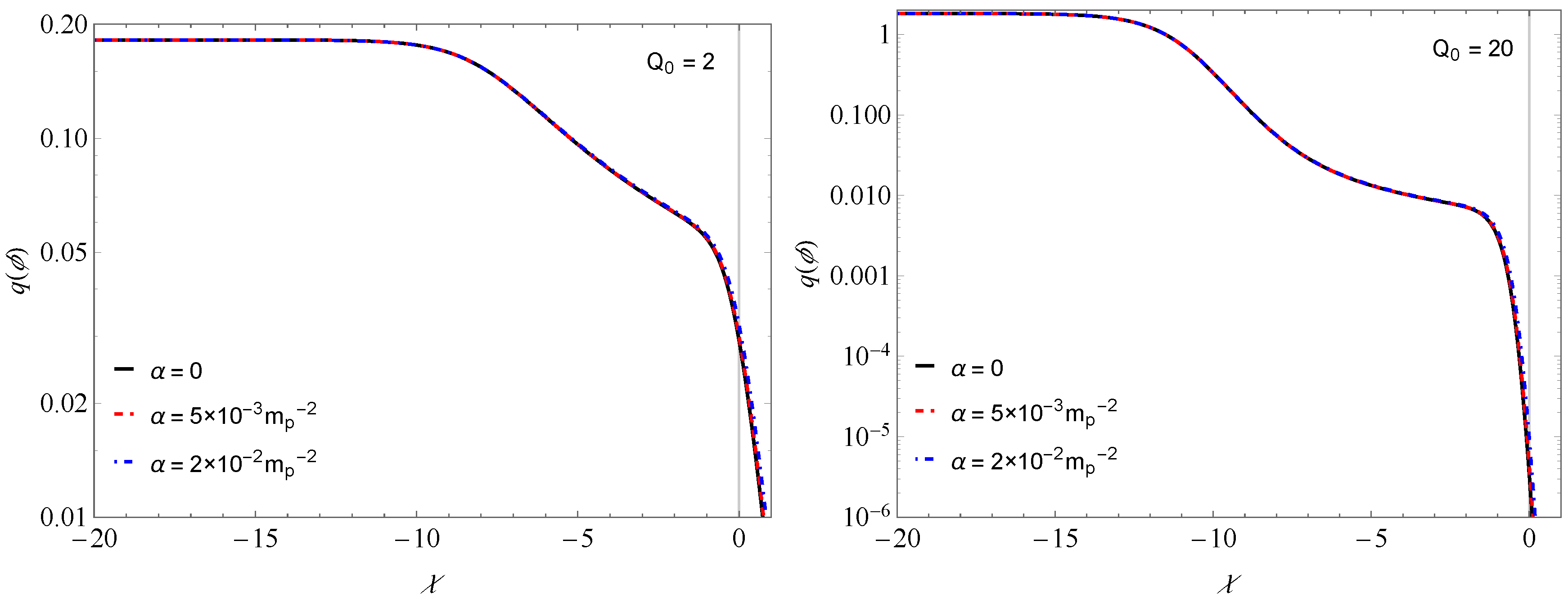
5.4. The Running of
5.5. The Energy Densities , , and
6. Discussions
7. Conclusions
Author Contributions
Funding
Data Availability Statement
Conflicts of Interest
References
- Riess, A.G.; Filippenko, A.V.; Challis, P.; Clocchiatti, A.; Diercks, A.; Garnavich, P.M.; Gilliland, R.L.; Hogan, C.J.; Jha, S.; Kirshner, R.P.; et al. Observational evidence from supernovae for an accelerating universe and a cosmological constant. Astron. J. 1998, 116, 1009. [Google Scholar] [CrossRef]
- Perlmutter, S.; Aldering1, G.; Goldhaber, G.; Knop, R.A.; Nugent, P.; Castro, P.G.; Deustua1, S.; Fabbro, S.; Goobar, A.; Groom, D.E.; et al. Measurements of Ω and λ from 42 High-Redshift Supernovae. Astrophys. J. 1999, 517, 565. [Google Scholar] [CrossRef]
- Koivisto, T.; Mota, D.F. Dark energy anisotropic stress and large scale structure formation. Phys. Rev. D 2006, 73, 083502. [Google Scholar] [CrossRef]
- Daniel, S.F.; Caldwell, R.R.; Cooray, A.; Melchiorri, A. Large scale structure as a probe of gravitational slip. Phys. Rev. D 2008, 77, 103513. [Google Scholar] [CrossRef]
- Komatsu, E.; Kogut, A.; Nolta, M.R.; Bennett, C.L.; Halpern, M.; Hinshaw, G.; Jarosik, N.; Limon, M.; Meyer, S.S.; Page, L.; et al. First-year Wilkinson microwave anisotropy probe (wmap)* observations: Tests of Gaussianity. Astrophys. J. Suppl. 2003, 148, 119–134. [Google Scholar] [CrossRef]
- Spergel, D.N.; et al. [WMAP Collaboration]. First-Year Wilkinson Microwave Anisotropy Probe (WMAP)* Observations: Determination of Cosmological Parameters. Astrophys. J. Suppl. 2003, 148, 175. [Google Scholar] [CrossRef]
- Hinshaw, G.; Larson, D.; Komatsu, E.; Spergel, D.N.; Bennett, C.; Dunkley, J.; Nolta, M.R.; Halpern, M.; Hill, R.S.; Odegard, N.; et al. Nine-year Wilkinson Microwave Anisotropy Probe (WMAP) observations: Cosmological parameter results. Astrophys. J. Suppl. 2013, 208, 19. [Google Scholar] [CrossRef]
- Caldwell, R.R.; Doran, M. Cosmic microwave background and supernova constraints on quintessence: Concordance regions and target models. Phys. Rev. D 2004, 69, 103517. [Google Scholar] [CrossRef]
- Huang, Z.Y.; Wang, B.; Abdalla, E.; Su, R.K. Holographic explanation of wide-angle power correlation suppression in the cosmic microwave background radiation. J. Cosmol. Astropart. Phys. 2006, 0605, 013. [Google Scholar] [CrossRef]
- Eisenstein, D.J.; Zehavi, I.; Hogg, D.W.; Scoccimarro, R.; Blanton, M.R.; Nichol, R.C.; Scranton, R.; Seo, H.J.; Tegmark, M.; Zheng, Z.; et al. Detection of the baryon acoustic peak in the large-scale correlation function of SDSS luminous red galaxies. Astrophys. J. 2005, 633, 560. [Google Scholar] [CrossRef]
- Percival, W.J.; Reid, B.A.; Eisenstein, D.J.; Bahcall, N.A.; Budavari, T.; Frieman, J.A.; Fukugita, M.; Gunn, J.E.; Ivezić, Ž.; Knapp, G.R.; et al. Baryon acoustic oscillations in the Sloan Digital Sky Survey data release 7 galaxy sample. Mon. Not. R. Astron. Soc. 2010, 401, 2148. [Google Scholar] [CrossRef]
- Abbott, B.P.; et al. [LIGO Scientific Collaboration and Virgo Collaboration]. Observation of Gravitational Waves from a Binary Black Hole Merger. Phys. Rev. Lett. 2016, 116, 061102. [Google Scholar] [CrossRef]
- Padmanabhan, T. Dark energy and gravity. Gen. Relativ. Gravit. 2008, 40, 529–564. [Google Scholar] [CrossRef]
- Frieman, J.; Turner, M.; Huterer, D. Dark Energy and the Accelerating Universe. Ann. Rev. Astron. Astrophys. 2008, 46, 385–432. [Google Scholar] [CrossRef]
- Martin, J. Quintessence: A mini-review. Mod. Phys. Lett. A 2008, 23, 1252–1265. [Google Scholar] [CrossRef]
- Caldwell, R.R.; Kamionkowski, M. The Physics of Cosmic Acceleration. Ann. Rev. Nucl. Part. Sci. 2009, 59, 397–429. [Google Scholar] [CrossRef]
- Silvestri, A.; Trodden, M. Approaches to Understanding Cosmic Acceleration. Rep. Prog. Phys. 2009, 72, 096901. [Google Scholar] [CrossRef]
- Bamba, K.; Capozziello, S.; Nojiri, S.; Odintsov, S.D. Dark energy cosmology: The equivalent description via different theoretical models and cosmography tests. Astrophys. Space Sci. 2012, 342, 155–228. [Google Scholar] [CrossRef]
- Li, M.; Li, X.-D.; Wang, S.; Wang, Y. Dark Energy: A Brief Review. Front. Phys. 2013, 8, 828–846. [Google Scholar] [CrossRef]
- Sami, M.; Myrzakulov, R. Late time cosmic acceleration: ABCD of dark energy and modified theories of gravity. Int. J. Mod. Phys. D 2016, 25, 1630031. [Google Scholar] [CrossRef]
- Peebles, P.J.E.; Ratra, B. The Cosmological Constant and Dark Energy. Rev. Mod. Phys. 2003, 75, 559–606. [Google Scholar] [CrossRef]
- Padmanabhan, T. Cosmological constant: The Weight of the vacuum. Phys. Rep. 2003, 380, 235–320. [Google Scholar] [CrossRef]
- Sahni, V. The Cosmological constant problem and quintessence. Class. Quant. Grav. 2002, 19, 3435–3448. [Google Scholar] [CrossRef]
- Velten, H.E.; Vom Marttens, R.F.; Zimdahl, W. Aspects of the cosmological “coincidence problem”. Eur. Phys. J. C 2014, 74, 3160. [Google Scholar] [CrossRef]
- Tsujikawa, S. Quintessence: A Review. Class. Quant. Grav. 2013, 30, 214003. [Google Scholar] [CrossRef]
- Buchdahl, H.A. Non-linear Lagrangians and cosmological theory. Mon. Not. R. Astron. Soc. 1970, 150, 1–8. [Google Scholar] [CrossRef]
- Sotiriou, T.P.; Faraoni, V. f(r) theories of gravity. Rev. Mod. Phys. 2010, 82, 451. [Google Scholar] [CrossRef]
- Nojiri, S.; Odintsov, S.D. Unified cosmic history in modified gravity: From F(R) theory to Lorentz non-invariant models. Phys. Rept. 2011, 505, 59–144. [Google Scholar] [CrossRef]
- Nojiri, S.; Odintsov, S.D.; Oikonomou, V.K. Modified Gravity Theories on a Nutshell: Inflation, Bounce and Late-time Evolution. Phys. Rept. 2017, 692, 1–104. [Google Scholar] [CrossRef]
- Starobinsky, A.A. A new type of isotropic cosmological models without singularity. Phys. Lett. B 1980, 91, 99–102. [Google Scholar] [CrossRef]
- Carroll, S.M.; Duvvuri, V.; Trodden, M.; Turner, M.S. Is cosmic speed-up due to new gravitational physics? Phys. Rev. D 2004, 70, 043528. [Google Scholar] [CrossRef]
- Nojiri, S.; Odintsov, S.D. Modified gravity with negative and positive powers of the curvature: Unification of the inflation and of the cosmic acceleration. Phys. Rev. D 2003, 68, 123512. [Google Scholar] [CrossRef]
- Capozziello, S.; Cardone, V.F.; Carloni, S.; Troisi, A. Curvature quintessence matched with observational data. Int. J. Mod. Phys. D 2003, 12, 1969–1982. [Google Scholar] [CrossRef]
- Dzhunushaliev, V.; Folomeev, V.; Kleihaus, B.; Kunz, J. Modified gravity from the quantum part of the metric. Eur. Phys. J. C 2014, 74, 2743. [Google Scholar] [CrossRef]
- Yang, R. Effects of quantum fluctuations of metric on the universe. Phys. Dark Universe 2016, 13, 87. [Google Scholar] [CrossRef]
- Liu, X.; Harko, T.; Liang, S.D. Cosmological implications of modified gravity induced by quantum metric fluctuations. Eur. Phys. J. C 2016, 76, 420. [Google Scholar] [CrossRef]
- Harko, T.; Lobo, F.S.; Nojiri, S.I.; Odintsov, S.D. f(R,T) gravity. Phys. Rev. D 2011, 84, 024020. [Google Scholar] [CrossRef]
- Shabani, H.; Farhoudi, M. f(R,T) cosmological models in phase space. Phys. Rev. D 2013, 88, 044048. [Google Scholar] [CrossRef]
- Xu, M.X.; Harko, T.; Liang, S.D. Quantum Cosmology of f(R,T) gravity. Eur. Phys. J. C 2016, 76, 449. [Google Scholar] [CrossRef]
- Moraes, P.H.R.S.; Sahoo, P.K. The simplest non-minimal matter-geometry coupling in the f(R,T) cosmology. Eur. Phys. J. C 2017, 77, 480. [Google Scholar] [CrossRef]
- Shabani, H.; Ziaie, A.H. Bouncing cosmological solutions from f(R,T) gravity. Eur. Phys. J. C 2018, 78, 397. [Google Scholar] [CrossRef]
- Debnath, P.S. Bulk viscous cosmological model in f(R,T) theory of gravity. Int. J.Geom. Meth. Mod. Phys. 2019, 16, 1950005. [Google Scholar] [CrossRef]
- Bhattacharjee, S.; Sahoo, P. Comprehensive analysis of a non-singular bounce in f(R,T) gravitation. Phys. Dark Universe 2020, 28, 100537. [Google Scholar] [CrossRef]
- Bhattacharjee, S.; Santos, J.R.L.; Moraes, P.H.R.S.; Sahoo, P.K. Inflation in f(R,T) gravity. Eur. Phys. J. Plus 2020, 135, 576. [Google Scholar] [CrossRef]
- Gamonal, M. Slow-roll inflation in f(R,T) gravity and a modified Starobinsky-like inflationary model. Phys. Dark Universe 2021, 31, 100768. [Google Scholar] [CrossRef]
- Witten, E. Some properties of O (32) superstrings. Phys. Lett. B 1984, 149, 351–356. [Google Scholar] [CrossRef]
- Witten, E. String theory dynamics in various dimensions. Nucl. Phys. B 1995, 443, 85–126. [Google Scholar] [CrossRef]
- Damour, T.; Polyakov, A.M. The String dilaton and a least coupling principle. Nucl. Phys. B 1994, 423, 532. [Google Scholar] [CrossRef]
- Gasperini, M. Dilatonic interpretation of quintessence? Phys. Rev. D 2001, 64, 043510. [Google Scholar] [CrossRef]
- Gasperini, M.; Piazza, F.; Veneziano, G. Quintessence as a runaway dilaton. Phys. Rev. D 2001, 65, 023508. [Google Scholar] [CrossRef]
- Veneziano, G. Large N bounds on, and compositeness limit of, gauge and gravitational interactions. J. High Energy Phys. 2002, 6, 051. [Google Scholar] [CrossRef]
- Taylor, T.R.; Veneziano, G. Dilaton couplings at large distances. Phys. Lett. B 1988, 213, 459. [Google Scholar] [CrossRef]
- Poplawski, N.J. A Lagrangian description of interacting dark energy. arXiv 2006, arXiv:gr-qc/0608031. [Google Scholar]
- Fischbach, E.; Talmadge, C. Six years of the fifth force. Nature 1992, 356, 207–215. [Google Scholar] [CrossRef]
- Gasperini, M. On the response of gravitational antennas to dilatonic waves. Phys. Lett. B 1999, 470, 67–72. [Google Scholar] [CrossRef]
- Riess, A.G.; Casertano, S.; Yuan, W.; Macri, L.M.; Scolnic, D. Large Magellanic Cloud Cepheid Standards Provide a 1% Foundation for the Determination of the Hubble Constant and Stronger Evidence for Physics beyond ΛCDM. Astrophys. J. 2019, 876, 85. [Google Scholar] [CrossRef]
- Riess, A.G.; Yuan, W.; Macri, L.M.; Scolnic, D.; Brout, D.; Casertano, S.; Jones, D.O.; Murakami, Y.; Anand, G.S.; Breuval, L.; et al. A Comprehensive Measurement of the Local Value of the Hubble Constant with 1 km s−1 Mpc−1 Uncertainty from the Hubble Space Telescope and the SH0ES Team. Astrophys. J. Lett. 2022, 934, L7. [Google Scholar] [CrossRef]
- Aghanim, N.; et al. [Planck]. Planck 2018 results. VI. Cosmological parameters. Astron. Astrophys. 2020, 641, A6, Erratum in Astron. Astrophys. 2021, 652, C4. [Google Scholar] [CrossRef]
- Ambjorn, J.; Watabiki, Y. Easing the Hubble constant tension. Mod. Phys. Lett. A 2022, 37, 2250041. [Google Scholar] [CrossRef]
- Santos, J.R.L.; da Costa, S.S.; Santos, R.S. Cosmological models for f(R,T)-Λ(ϕ) gravity. Phys. Dark Univ. 2023, 42, 101356. [Google Scholar] [CrossRef]


| Experiments | |||
|---|---|---|---|
| Riess et al. 2019 [56] | km s−1 Mpc−1 | − | − |
| Planck 2018 [58] | km s−1 Mpc−1 | − | − |
| Scenarios | |||
| I | km s−1 Mpc−1 | 2 | |
| II | km s−1 Mpc−1 | 0 | 2–20 |
| III | km s−1 Mpc−1 | 2–20 |
| 0.271 | 0.049 | 0.679 | 0 | 2 | |
| 0.219 | 0.040 | 0.740 | 0 | 20 | |
| 0.302 | 0.056 | 0.636 | 2 | ||
| 0.266 | 0.047 | 0.701 | 20 |
| 3391 | 67.0 | 0 | 2 | |
| 3346.6 | 74.4 | 0 | 20 | |
| 604.1 | 68.1 | 2 | ||
| 425.6 | 75.5 | 20 |
Disclaimer/Publisher’s Note: The statements, opinions and data contained in all publications are solely those of the individual author(s) and contributor(s) and not of MDPI and/or the editor(s). MDPI and/or the editor(s) disclaim responsibility for any injury to people or property resulting from any ideas, methods, instructions or products referred to in the content. |
© 2024 by the authors. Licensee MDPI, Basel, Switzerland. This article is an open access article distributed under the terms and conditions of the Creative Commons Attribution (CC BY) license (https://creativecommons.org/licenses/by/4.0/).
Share and Cite
Brito, F.A.; Borges, C.H.A.B.; Campos, J.A.V.; Costa, F.G.
Weak Coupling Regime in Dilatonic
Brito FA, Borges CHAB, Campos JAV, Costa FG.
Weak Coupling Regime in Dilatonic
Brito, Francisco A., Carlos H. A. B. Borges, José A. V. Campos, and Francisco G. Costa.
2024. "Weak Coupling Regime in Dilatonic