Article

Re-Examination of the Effect of Pairing Gaps on Gamow–Teller Strength Distributions and β-Decay Rates

1
Department of Physics, University of Wah, Quaid Avenue, Wah Cantt 47040, Pakistan
2
Department of Physics, University of Jhang, Jhang 35400, Pakistan
*
Author to whom correspondence should be addressed.
These authors contributed equally to this work.
Universe 2024, 10(3), 128; https://doi.org/10.3390/universe10030128
Submission received: 17 December 2023 / Revised: 31 January 2024 / Accepted: 4 March 2024 / Published: 6 March 2024

Abstract

:
β -decay is one of the key factors for understanding the r-process and evolution of massive stars. The Gamow–Teller (GT) transitions drive the β -decay process. We employ the proton–neutron quasiparticle random phase approximation (pn-QRPA) model to calculate terrestrial and stellar β -decay rates for 50 top-ranked nuclei possessing astrophysical significance according to a recent survey. The model parameters of the pn-QRPA model affect the predicted results of β -decay. The current study investigates the effect of nucleon–nucleon pairing gaps on charge-changing transitions and the associated β decay rates. Three different values of pairing gaps, namely TF, 3TF, and 5TF, were used in our investigation. It was concluded that both GT strength distributions and half-lives are sensitive to pairing gap values. The 3TF pairing gap scheme, in our chosen nuclear model, resulted in the best prediction with around 80% of the calculated half-lives within a factor 10 of the measured ones. The 3TF pairing scheme also led to the calculation of the biggest β -decay rates in stellar matter.

1. Introduction

The nuclear reactions mediated by weak interactions play a crucial role in the presupernova evolution of massive stars [1]. The β ± decay, electron, and positron capture are the fundamental weak interaction processes that occur during the presupernova phases. The β -decay and electron capture are transformations that produce (anti)neutrinos. A change of lepton-to-baryon fraction ( Y e ) of the core matter affects the dynamics of collapse and subsequent explosion of the massive stars [2,3]. Two important parameters to determine the dynamics of core-collapse are the time rate of Y e and the entropy of the core material [4]. The weak interaction-mediated rates play an important role in stellar processes including hydrostatic burning and pre-supernova evolution of massive stars. The study of stellar weak interaction rates is a key area for investigation due to its significant contribution in understanding of pre-supernova evolution of massive stars. The core-collapse simulation depends on reliable computation of ground- and excited-states Gamow–Teller (GT) strength functions [4]. A substantial number of unstable nuclei are present in the core with varying abundances. Weak interactions of these nuclei in stellar matter may contribute to a better understanding of the complex dynamics of core-collapse. Once an iron core develops in a giant star’s later stages of evolution, there is no more fuel available to start a new burning cycle. Lepton capture and photo-disintegration processes lead to the core’s increasing instability and eventual collapse. The number of electrons available for pressure support is reduced by the electron capture process, whereas degeneracy pressure is enhanced during β decays [5]. Few recent papers highlighting the impact of β -decays on late stellar evolution include Refs. [6,7,8,9,10].
Determination of β -decay rates is also required for the nucleosynthesis (s-, p-, and r-) processes [11,12]. The r-process synthesizes half of the elements heavier than iron [12]. The site of r-process remains uncertain to date [13,14,15]. Pre-requisites include high neutron densities and core temperatures. In recent years, much experimental work has been conducted to study the nuclear properties of exotic nuclei. Since the majority of these nuclei cannot be created under lab conditions, microscopic calculations of stellar weak-decay properties have gained importance in our quest to comprehend stellar processes. Numerous computations have focused on the mechanisms underlying stellar development and nucleosynthesis (e.g., [16,17,18,19,20,21]).
The β -decay half-lives were estimated with the help of gross theory [18]. With the advancement of computing and new technologies, the calculation of ground and excited states GT strength distributions gained the attention of many researchers. The charge-changing reaction rates in the stellar environment were estimated using several nuclear models. Fuller, Fowler, and Newman made the first substantial effort to compute the astrophysical rates using the independent particle model (IPM) [22]. To enhance the reliability of their calculation, they took into account the measurable data that were available at the time. Later, many other sophisticated nuclear models were used to calculate reduced transition probabilities of GT transitions. Noticeable mentions include the shell model Monte Carlo technique (e.g., [23]), thermal quasiparticle random-phase approximation, QRPA (e.g., [24,25,26]), density functional theory (e.g., [19]), the Hartree–Fock–Bogoliubov method (e.g., [20]), and the shell model (e.g., [21]).
The current study investigates the effect of pairing gaps on the calculated GT strength functions and the associated β -decay rates under terrestrial and stellar conditions. The β -decay properties were studied using the quasiparticle random phase approximation model with a separable multi-shell schematic and a separable interaction in addition to the axially symmetric-deformed mean-field calculation. Previously, similar investigations were performed separately for s d - [27] and f p -shell nuclei [28,29]. Recently, a list was published detailing the top 50 nuclei capable of electron capturing and β decaying, which have the largest effect on Y e from conditions after silicon core burning to those preceding core collapse and neutrino trapping [30]. This investigation led to the identification of the most important weak interaction nuclei in the presupernova evolution of massive stars. To achieve this goal, an ensemble containing 728 nuclei in the mass range of A = (1–100) was considered. The idea was to sort nuclei having the largest effect on Y e following silicon core burning, by averaging the contribution from each nucleus to Y e ˙ (the time rate of change of the lepton fraction) across the entire selected stellar trajectory. In the current project, we specifically focus on the top-ranked 50 nuclei as per the findings of Ref. [30] (with β as the dominant decay mode [31]), and study the effect of pairing gaps on the β -decay properties of these nuclei.
Pairing gaps are some of the most important parameters in the pn-QRPA model. We should note that the present investigation includes neutron–neutron and proton–proton pairing correlations, which only have isovector contributions. For the isoscalar part, one has to include the neutron–proton ( n p ) pairing correlations, which is not considered in the present manuscript. The current pn-QRPA model is limited as it ignores the neutron–proton n p pairing effect and the incorporation of n p pairing may be focused on in a future assignment. Such kinds of calculations were performed earlier by the author in Ref. [32], albeit only for N = Z + 2 nuclei. The conclusions of their study stated that isoscalar interaction behaves in a fashion similar to the tensor force interaction. The calculations presented in Ref. [32] showed that the tensor force shifts the GT peak to lower excitation energies. Incorporating the tensor force may result in lower centroid values of the calculated GT strength distributions and could lead to higher values of calculated β -decay rates. To compensate, the same effect of shifting the calculated β strength to lower excitation energies in the current pn-QRPA model was achieved by incorporating particle–particle forces (see Section 2 of Ref. [33]). The pairing energy of identical nucleons in even–even isotopes can be estimated using a variety of methods based on the masses of neighboring nuclei, but despite extensive study, the question of which relation most closely approximates the pairing interaction remains open for debate [34,35,36,37]. We chose to employ three different recipes for the calculation of pairing gaps in our investigation. Details follow in the next section.
This paper is organized as follows: The theoretical framework used for calculations is described in Section 2. Section 3 presents the discussion of our investigation. Finally, the summary and concluding remarks of the present work are presented in Section 4.

2. Formalism

The Hamiltonian of the current pn-QRPA model is given as follows:
H p n Q R P A = H s p + V p a i r i n g + V G T p h + V G T p p ,
where H s p , V p a i r i n g , V G T p h , and V G T p p denote the single-particle Hamiltonian, pairing forces for the BCS calculation, and particle–hole ( p h ) and particle–particle ( p p ) interactions for GT strength, respectively. The single-particle eigenfunctions and eigenvalues were computed using the Nilsson model [38]. Other parameters essential for the solution of Equation (1) are nuclear deformation, the Nilsson potential parameter (NPP), Q-values, pairing gaps, and the GT force parameters. The Q-value for β decay was calculated using the following:
Q = [ m ( Z A P ) m ( Z + 1 A D ) ] c 2 ,
where P is the parent nucleus, D is the daughter nucleus, and m is the nuclear mass.
The nuclear deformation parameter ( β 2 ) was determined using the following formula:
β 2 = 125 ( Q 2 ) 1.44 ( A ) 2 / 3 ( Z ) ,
where Q 2 is the electric quadrupole moment taken from [39]. The NPPs were chosen from [40]. The Nilsson oscillator constant was taken as ћ ω = 41 / A + 1 / 3 in units of MeV, similar for neutrons and protons. Q-values were determined using the recent mass compilation [31].
The pairing gaps between nucleons were chosen using three different formulae. The first formula is used the most in the literature [33,41,42]. It has the same value for neutron–neutron and proton–proton pairings. It is given by the following:
Δ n n = Δ p p = 12 / A .
This is the traditionally used formula for the calculation of pairing gaps. The second formula contains three terms and is based on the separation energies of neutrons and protons. It is given by the following:
Δ n n = 1 8 ( 1 ) A Z + 1 [ 2 S n ( A + 1 , Z ) 4 S n ( A , Z ) + 2 S n ( A 1 , Z ) ]
Δ p p = 1 8 ( 1 ) 1 + Z [ 2 S p ( A + 1 , Z + 1 ) 4 S p ( A , Z ) + 2 S p ( A 1 , Z 1 ) ] .
The third recipe contains five terms and is a function of the binding energies of the nucleons. It is given by the following:
Δ n n = 1 16 [ 2 B ( Z , N 2 ) 8 B ( Z , N 1 ) + 12 B ( Z , N ) 8 B ( Z , N + 1 ) + 2 B ( Z , N + 2 ) ]
Δ p p = 1 16 [ 2 B ( Z 2 , N ) 8 B ( Z 1 , N ) + 12 B ( Z , N ) 8 B ( Z + 1 , N ) + 2 B ( Z + 2 , N ) ] .
The values of binding energies were taken from Ref. [43]. Henceforth, in this text, we will refer to the first formula of pairing gaps as TF (one-term or a traditional formula), the second as 3TF (three-term formula), and the last formula as 5TF (five-term formula).
The spherical nucleon basis represented by ( c j m and c j m ), with angular momentum j, and m as its z-component, was transformed into a deformed basis ( d m α , d m α ) using the following transformation:
d m α = Σ j D j m α c j m ,
where c and d are the particle creation operators in the spherical and deformed bases, respectively. The transformation matrix, D, denotes a set of Nilsson eigenfunctions, and α represents the additional quantum numbers. Later, we used the Bogoliubov transformation to introduce the quasiparticle basis ( a m α , a m α )
a m α = u m α d m α v m α d m ¯ α
a m ¯ α = u m α d m ¯ α + v m α d m α ( m > 0 ) ,
where m ¯ represents the time-reversed state of m. The occupation amplitudes satisfied the condition v m α 2 + u m α 2 = 1, and were computed using the BCS equations with pairing gaps given in Equations (4)–(8). The pn-QRPA theory deals with quasiparticle states of the proton–neutron systems and the correlations between them. The ground state is a vacuum for QRPA phonon, Γ ^ ω | QRPA > = 0 , with the phonon creation operator defined by the following:
Γ ^ ω ( μ ) = π , ν X ω π ν ( μ ) a ^ π a ^ ν ¯ Y ω π ν ( μ ) a ^ ν a ^ π ¯ ,
where ν and π , respectively, denote the single quasiparticle states of neutrons and protons. The sum runs over all possible π ν -pairs, satisfying μ = m π m ν = (0, ±1). The forward-going ( X ω ) and backward-going ( Y ω ) amplitudes are eigenvectors, whereas, energy ( ω ) denotes the eigenvalues of the well-known (Q)RPA equation:
M N N M X Y = ω X Y .
The solution of Equation (13) was obtained for each projection value ( μ = 0 , ± 1 ). Matrix elements M and N were determined using the following:
M π ν , π ν = δ π ν , π ν ( ε π + ε ν ) + V π ν , π ν p p ( v π v ν v π v ν + u π u ν u π u ν ) + V π ν , π ν p h ( v π u ν v π u ν + u π v ν u π v ν ) ,
N π ν , π ν = V π ν , π ν p p ( u π u ν v π v ν + v π v ν u π u ν ) V π ν , π ν p h ( v π u ν u π v ν + u π v ν v π u ν ) ,
with
V π ν , π ν p p = V π ν ¯ , π ν ¯ ,
V π ν , π ν p h = V π ν , π ν .
The quasiparticle energies ( ε π , ε ν ) were obtained from the BCS calculations. We used separable GT residual forces, namely, particle–hole ( p h ) and particle–particle ( p p ) forces in our calculation. We took the p p GT force as follows:
V G T p p = 2 κ μ ( 1 ) μ P ^ μ P ^ μ ,
where
P ^ μ = j π m π j ν m ν j ν m ν | ( σ μ τ ) | j π m π ( 1 ) l ν + j ν m ν c ^ j π m π c ^ j ν m ν ,
and the p h GT force as follows:
V G T p h = 2 χ μ ( 1 ) μ R ^ μ R ^ μ ,
where
R ^ μ = j π m π j ν m ν j π m π | σ μ τ | j ν m ν c ^ j π m π c ^ j ν m ν ,
where χ and κ are the p p and p h GT force parameters, respectively. With the use of separable GT forces in our calculation, the RPA matrix equation reduced to a fourth-order algebraic equation. The method to determine the roots of these equations can be seen from [44]. This simplification saved the computational time when compared to the full diagonalization of the nuclear Hamiltonian (Equation (1)).
In the RPA formalism, excitations from the ground state ( J π = 0 + ) of an even–even nucleus are considered. The ground state of an odd–odd (odd-A) parent nucleus is expressed as a proton–neutron quasiparticle pair (one-quasiparticle) state of the smallest energy. Then two possible transitions are the phonon excitations (where the quasiparticle merely plays the role of a spectator) and the transition of the quasiparticle itself. In the latter case, correlations of phonons to the quasiparticle transitions were treated using first-order perturbation theory [24].
We next present quasiparticle transitions, the construction of phonon-related multi-quasiparticle states (representing nuclear-excited levels of even–even, odd-A, and odd–odd nuclei), and formulae for GT transitions within the current model using the recipe given in [44]. The occupation amplitudes of the quasiparticle states were calculated within BCS formalism using three different pairing gap values. The phonon-correlated one-quasiparticle states were defined by the following:
| π c o r r = a π | + ν , ω a ν A ω ( μ ) | | [ a ν A ω ( μ ) ] H 31 a π | × E π ( ν , ω ) ,
| ν c o r r = a ν | + π , ω a π A ω ( μ ) | | [ a π A ω ( μ ) ] H 31 a ν | × E ν ( π , ω ) ,
with
E a ( b , ω ) = 1 ϵ a ϵ b ω a , b = π , ν ,
and
H 31 = V π ν , π ¯ ν ( u π u ν v π u ν v π v ν u π v ν ) ( a π a ν a π a ν + h . c . ) + V π ν , π ν ¯ ( v π v ν v π u ν u π u ν u π v ν ) ( a π a ν a ν a π + h . c . ) ,
where h . c . stands for Hermitian conjugate. The terms E a ( b , ω ) can be modified to prevent the singularity in the transition amplitude caused by the first-order perturbation of the odd-particle wave function. The first term in Equations (22) and (23) denotes the proton (neutron) quasiparticle state, while the second term denotes RPA-correlated phonons admixed with quasiparticle-phonon-coupled Hamiltonian H 31 , which was accomplished by the Bogoliubov transformation from separable p p and p h GT interaction forces. The summation applies to all phonon states and neutron (proton) quasiparticle states, satisfying m π m ν = μ with π π π ν = 1 . The calculation of quasiparticle transition amplitudes for correlated states can be found in [45]. The amplitudes of GT transitions in terms of separable forces are as follows:
< π c o r r | τ σ μ | ν c o r r > = q π ν U + 2 χ [ q π ν U ω ( Z ω 2 E π ( ν , ω ) + Z ω + 2 E ν ( π , ω ) ) q π ν V ω Z ω Z ω + ( E π ( ν , ω ) + E ν ( π , ω ) ) ] + 2 κ [ q π ν ω ( Z ω Z ω E π ( ν , ω ) Z ω + Z ω + + E ν ( π , ω ) ) q ˜ π ν ω ( Z ω Z ω + + E π ( ν , ω ) Z ω + Z ω E ν ( π , ω ) ) ] ,
< π c o r r | τ + σ μ | ν c o r r > = q π ν V + 2 χ [ q π ν V ω ( Z ω + 2 E π ( ν , ω ) + Z ω 2 E ν ( π , ω ) ) q π ν U ω Z ω Z ω + ( E π ( ν , ω ) + E ν ( π , ω ) ) ] + 2 κ [ q ˜ π ν ω ( Z ω + Z ω + + E π ( ν , ω ) Z ω Z ω E ν ( π , ω ) ) q π ν ω ( Z ω + Z ω E π ( ν , ω ) Z ω Z ω + + E ν ( π , ω ) ) ] ,
< ν c o r r | τ ± σ μ | π c o r r > = ( 1 ) μ < π c o r r | τ σ μ | ν c o r r > .
In Equations (26)–(28), σ μ , and τ ± are spin and iso-spin type operators, respectively, and other symbols, q π ν ( q ˜ π ν ), q π ν U ( q π ν V ), Z ω ( Z ω + ) and Z ω ( Z ω + + ), are defined as follows:
q π ν = f π ν u π v ν , q π ν U = f π ν u π u ν , q ˜ π ν = f π ν v π u ν , q π ν V = f π ν v π v ν Z ω = π , ν ( X ω π ν q π ν Y ω π ν q ˜ π ν ) , Z ω + = π , ν ( X ω π ν q ˜ π ν Y ω π ν q π ν ) , Z ω = π , ν ( X ω π ν q π ν U + Y ω π ν q π ν V ) , Z ω + + = π ν ( X ω π , ν q π ν V + Y ω π ν q π ν U ) .
The terms X ω π ν and Y ω π ν were defined earlier and other symbols have the usual meanings. The idea surrounding quasiparticle transitions with first-order phonon correlations can be extended to an odd–odd parent nucleus. The ground state is assumed to be a proton–neutron quasiparticle pair state of the smallest energy. The GT transitions of the quasiparticle led to two-proton or two-neutron quasiparticle states in the even–even daughter nucleus. The two quasiparticle states were constructed with phonon correlations, given by the following:
| π ν c o r r > = a π a ν | > + 1 2 π 1 , π 2 , ω a π 1 a π 2 A ω ( μ ) | > × < | [ a π 1 a π 2 A ω ( μ ) ] H 31 a π a ν | > E π ν ( π 1 π 2 , ω ) + 1 2 ν 1 , ν 2 , ω a ν 1 a ν 2 A ω ( μ ) | > × < | [ a ν 1 a ν 2 A ω ( μ ) ] H 31 a π a ν | > E π ν ( ν 1 ν 2 , ω ) ,
< π 1 π 2 c o r r | = a π 1 a π 2 | > + π , ν , ω a π a ν A ω ( μ ) | > × < | [ a π a ν A ω ( μ ) ] H 31 a π 1 a π 2 | > E π 1 π 2 ( π ν , ω ) ,
< ν 1 ν 2 c o r r | = a ν 1 a ν 2 | > + π , ν , ω a π + a ν A ω ( μ ) | > × < | [ a π a ν A ω ( μ ) ] H 31 a ν 1 a ν 2 | > E ν 1 ν 2 ( π ν , ω ) ,
where
E a b ( c d , ω ) = 1 ( ϵ a + ϵ b ) ( ϵ c + ϵ d + ω ) <
where subscript index a (b) denotes π , π 1 and ν 1 ( ν , π 2 and ν 2 ) and c (d) denotes π , π 1 and ν 1 ( ν , π 2 and ν 2 ). The GT transition amplitudes between these states were reduced to those of one-quasiparticle states:
< π 1 π 2 c o r r | τ ± σ μ | π ν c o r r > = δ ( π 1 , π ) < π 2 c o r r | τ ± σ μ | ν c o r r > δ ( π 2 , π ) < π 1 c o r r | τ ± σ μ | ν c o r r > ,
< ν 1 ν 2 c o r r | τ ± σ μ | π ν c o r r > = δ ( ν 2 , ν ) < ν 1 c o r r | τ ± σ μ | π c o r r > δ ( ν 1 , ν ) < ν 2 c o r r | τ ± σ μ | π c o r r > ,
by ignoring second-order terms in the correlated phonons. For odd–odd parent nuclei, QRPA phonon excitations are also possible, where the quasiparticle pairs act as spectators in the same single quasiparticle shells. The nuclear-excited states can be constructed as phonon-correlated multi-quasiparticle states. The transition amplitudes between multi-quasiparticle states can be reduced to those of one-quasiparticle states, as described below.
Excited levels of an even–even nucleus are two-proton quasiparticle states and two-neutron quasiparticle states. Transitions from these initial states to the final neutron–proton quasiparticle pair states are possible in the odd–odd daughter nuclei. The transition amplitudes can be reduced to correlated quasiparticle states by taking the Hermitian conjugate of Equations (34) and (35):
< π ν c o r r | τ ± σ μ | π 1 π 2 c o r r > = δ ( π , π 2 ) < ν c o r r | τ ± σ μ | π 1 c o r r > + δ ( π , π 1 ) < ν c o r r | τ ± σ μ | π 2 c o r r > ,
< π ν c o r r | τ ± σ μ | ν 1 ν 2 c o r r > = δ ( ν , ν 2 ) < π c o r r | τ ± σ μ | ν 1 c o r r > δ ( ν , ν 1 ) < π c o r r | τ ± σ μ | ν 2 c o r r > .
When a nucleus has an odd nucleon (a proton and/or a neutron), low-lying states are obtained by lifting the quasiparticle in the orbit of the smallest energy to higher-lying orbits. States of an odd-proton even-neutron nucleus were expressed by three-proton states or one-proton two-neutron states, corresponding to the excitation of a proton or a neutron, as follows:
| π 1 π 2 π 3 c o r r = a π 1 a π 2 a π 3 | + 1 2 π 1 , π 2 , ν , ω a π 1 a π 2 a ν A ω ( μ ) | × | [ a π 1 a π 2 a ν A ω ( μ ) ] H 31 a π 1 a π 2 a π 3 | E π 1 π 2 π 3 ( π 1 π 2 ν , ω ) ,
| π 1 ν 1 ν 2 c o r r = a π 1 a ν 1 a ν 2 | + 1 2 π 1 , π 2 , ν , ω a π 1 a π 2 a ν A ω ( μ ) | × | [ a π 1 a π 2 a ν A ω ( μ ) ] H 31 a π 1 a ν 1 a ν 2 | × E π 1 ν 1 ν 2 ( π 1 π 2 ν , ω ) + 1 6 ν 1 , ν 2 , ν 3 , ω a ν 1 a ν 2 a ν 3 A ω ( μ ) | × | [ a ν 1 a ν 2 a ν 3 A ω ( μ ) ] H 31 a π 1 a ν 1 a ν 2 | E π 1 ν 1 ν 2 ( ν 1 ν 2 ν 3 , ω ) ,
with the energy denominators of first-order perturbation:
E a b c ( d e f , ω ) = 1 ( ϵ a + ϵ b + ϵ c ϵ d ϵ e ϵ f ω ) ,
where subscripts represent π 1 , π 2 , π 3 , π , ν 1 , and ν 2 ( π 1 , π 2 , ν , ν 1 , ν 2 , and ν 2 ). These equations can be used to generate the three-quasiparticle states of odd protons and even neutrons by swapping the neutron and proton states, ν π and A ω ( μ ) A ω ( μ ) . Amplitudes of the quasiparticle transitions between the three-quasiparticle states were reduced to those for correlated one-quasiparticle states. For parent nuclei with an odd proton, we have the following:
π 1 π 2 ν 1 c o r r | τ ± σ μ | π 1 π 2 π 3 c o r r = δ ( π 1 , π 2 ) δ ( π 2 , π 3 ) ν 1 c o r r | τ ± σ μ | π 1 c o r r δ ( π 1 , π 1 ) δ ( π 2 , π 3 ) ν 1 c o r r | τ ± σ μ | π 2 c o r r + δ ( π 1 , π 1 ) δ ( π 2 , π 2 ) ν 1 c o r r | τ ± σ μ | π 3 c o r r ,
π 1 π 2 ν 1 c o r r | τ ± σ μ | π 1 ν 1 ν 2 c o r r = δ ( ν 1 , ν 2 ) [ δ ( π 1 , π 1 ) π 2 c o r r | τ ± σ μ | ν 1 c o r r δ ( π 2 , π 1 ) π 1 c o r r | τ ± σ μ | ν 1 c o r r ] δ ( ν 1 , ν 1 ) [ δ ( π 1 , π 1 ) π 2 c o r r | τ ± σ μ | ν 2 c o r r δ ( π 2 , π 1 ) π 1 c o r r | τ ± σ μ | ν 2 c o r r ] ,
ν 1 ν 2 ν 3 c o r r | τ ± σ μ | π 1 ν 1 ν 2 c o r r = δ ( ν 2 , ν 1 ) δ ( ν 3 , ν 2 ) ν 1 c o r r | τ ± σ μ | π 1 c o r r δ ( ν 1 , ν 1 ) δ ( ν 3 , ν 2 ) ν 2 c o r r | τ ± σ μ | π 1 c o r r + δ ( ν 1 , ν 1 ) δ ( ν 2 , ν 2 ) ν 3 c o r r | τ ± σ μ | π 1 c o r r ,
and for parent nuclei with an odd neutron, we have the following:
π 1 ν 1 ν 2 c o r r | τ ± σ μ | ν 1 ν 2 ν 3 c o r r = δ ( ν 1 , ν 2 ) δ ( ν 2 , ν 3 ) π 1 c o r r | τ ± σ μ | ν 1 c o r r δ ( ν 1 , ν 1 ) δ ( ν 2 , ν 3 ) π 1 c o r r | τ ± σ μ | ν 2 c o r r + δ ( ν 1 , ν 1 ) δ ( ν 2 , ν 2 ) π 1 c o r r | τ ± σ μ | ν 3 c o r r ,
π 1 ν 1 ν 2 c o r r | τ ± σ μ | π 1 π 2 ν 1 c o r r = δ ( π 1 , π 2 ) [ δ ( ν 1 , ν 1 ) ν 2 c o r r | τ ± σ μ | π 1 c o r r δ ( ν 2 , ν 1 ) ν 1 c o r r | τ ± σ μ | π 1 c o r r ] δ ( π 1 , π 1 ) [ δ ( ν 1 , ν 1 ) ν 2 c o r r | τ ± σ μ | π 2 c o r r δ ( ν 2 , ν 1 ) ν 1 c o r r | τ ± σ μ | π 2 c o r r ] ,
π 1 π 2 π 3 c o r r | τ ± σ μ | π 1 π 2 ν 1 c o r r = δ ( π 2 , π 1 ) δ ( π 3 , π 2 ) π 1 c o r r | τ ± σ μ | ν 1 c o r r δ ( π 1 , π 1 ) δ ( π 3 , π 2 ) π 2 c o r r | τ ± σ μ | ν 1 c o r r + δ ( π 1 , π 1 ) δ ( π 2 , π 2 ) π 3 c o r r | τ ± σ μ | ν 1 c o r r .
Low-lying states in an odd–odd nucleus were expressed in the quasiparticle picture by proton–neutron pair states (two quasiparticle states) or by states that were obtained by adding two-proton or two-neutron quasiparticles (four-quasiparticle states). Transitions from the former states were described earlier. Phonon-correlated four-quasiparticle states can be constructed similarly to the two- and three-quasiparticle states. Also in this case, transition amplitudes for the four-quasiparticle states were reduced to those for the correlated one-quasiparticle states, as follows:
< π 1 π 2 ν 1 ν 2 c o r r | τ ± σ μ | π 1 π 2 π 3 ν 1 c o r r > = δ ( ν 2 , ν 1 ) [ δ ( π 1 , π 2 ) δ ( π 2 , π 3 ) < ν 1 c o r r | τ ± σ μ | π 1 c o r r > δ ( π 1 , π 1 ) δ ( π 2 , π 3 ) < ν 1 c o r r | τ ± σ μ | π 2 c o r r > + δ ( π 1 , π 1 ) δ ( π 2 , π 2 ) < ν 1 c o r r | τ ± σ μ | π 3 c o r r > ] δ ( ν 1 , ν 1 ) [ δ ( π 1 , π 2 ) δ ( π 2 , π 3 ) < ν 2 c o r r | τ ± σ μ | π 1 c o r r > δ ( π 1 , π 1 ) δ ( π 2 , π 3 ) < ν 2 c o r r | τ ± σ μ | π 2 c o r r > + δ ( π 1 , π 1 ) δ ( π 2 , π 2 ) < ν 2 c o r r | τ ± σ μ | π 3 c o r r > ] ,
< π 1 π 2 π 3 π 4 c o r r | τ ± σ μ | π 1 π 2 π 3 ν 1 c o r r > = δ ( π 2 , π 1 ) δ ( π 3 , π 2 ) δ ( π 4 , π 3 ) < π 1 c o r r | τ ± σ μ | ν 1 c o r r > + δ ( π 1 , π 1 ) δ ( π 3 , π 2 ) δ ( π 4 , π 3 ) < π 2 c o r r | τ ± σ μ | ν 1 c o r r > δ ( π 1 , π 1 ) δ ( π 2 , π 2 ) δ ( π 4 , π 3 ) < π 3 c o r r | τ ± σ μ | ν 1 c o r r > + δ ( π 1 , π 1 ) δ ( π 2 , π 2 ) δ ( π 3 , π 3 ) < π 4 c o r r | τ ± σ μ | ν 1 c o r r > ,
< π 1 π 2 ν 1 ν 2 c o r r | τ ± σ μ | π 1 ν 1 ν 2 ν 3 c o r r > = δ ( π 1 , π 1 ) [ δ ( ν 1 , ν 2 ) δ ( ν 2 , ν 3 ) < π 2 c o r r | τ ± σ μ | ν 1 c o r r > δ ( ν 1 , ν 1 ) δ ( ν 2 , ν 3 ) < π 2 c o r r | τ ± σ μ | ν 2 c o r r > + δ ( ν 1 , ν 1 ) δ ( ν 2 , ν 2 ) < π 2 c o r r | τ ± σ μ | ν 3 c o r r > ] δ ( π 2 , π 1 ) [ δ ( ν 1 , ν 2 ) δ ( ν 2 , ν 3 ) < π 1 c o r r | τ ± σ μ | ν 1 c o r r > δ ( ν 1 , ν 1 ) δ ( ν 2 , ν 3 ) < π 1 c o r r | τ ± σ μ | ν 2 c o r r > + δ ( ν 1 , ν 1 ) δ ( ν 2 , ν 2 ) < π 1 c o r r | τ ± σ μ | ν 3 c o r r > ] ,
< ν 1 ν 2 ν 3 ν 4 c o r r | τ ± σ μ | π 1 ν 1 ν 2 ν 3 c o r r > = + δ ( ν 2 , ν 1 ) δ ( ν 3 , ν 2 ) δ ( ν 4 , ν 3 ) < ν 1 c o r r | τ ± σ μ | π 1 c o r r > δ ( ν 1 , ν 1 ) δ ( ν 3 , ν 2 ) δ ( ν 4 , ν 3 ) < ν 2 c o r r | τ ± σ μ | π 1 c o r r > + δ ( ν 1 , ν 1 ) δ ( ν 2 , ν 2 ) δ ( ν 4 , ν 3 ) < ν 3 c o r r | τ ± σ μ | π 1 c o r r > δ ( ν 1 , ν 1 ) δ ( ν 2 , ν 2 ) δ ( ν 3 , ν 3 ) < ν 4 c o r r | τ ± σ μ | π 1 c o r r > .
The antisymmetrization of the quasiparticles was duly taken into account for each of these amplitudes.
π 4 > π 3 > π 2 > π 1 , ν 4 > ν 3 > ν 2 > ν 1 , π 4 > π 3 > π 2 > π 1 , ν 4 > ν 3 > ν 2 > ν 1 .
The GT transitions were taken into account for the excited state of each phonon. It was assumed that the quasiparticle in the parent nucleus occupied the same orbit as the excited phonons.
The β -decay partial half-lives t 1 / 2 from the parent ground state were calculated using the following relation:
t p ( 1 / 2 ) = D f V ( Z , E , A ) B F ( ω ) + ( g V / g A ) 2 f A ( Z , E , A ) B G T ( ω ) ,
where E = ( Q ω ). The integrals of the available phase space for axial vector and vector transitions are denoted as f A ( Z , A , E ) and f V ( Z , A , E ) , respectively. The total β -decay half-lives were computed, including all transition probabilities to the states in the daughter within the Q window.
The stellar β -decay rates from the nth parent state to the mth daughter level were calculated using the following:
λ n m β = ln 2 f n m ( T , ρ , E f ) ( f t ) n m .
The term ( f t ) n m is linked to the reduced transition probabilities ( B n m ) of Fermi and GT transitions, as follows:
( f t ) n m = D / B n m ,
where
B n m = ( g A / g V ) 2 B ( G T ) n m + B ( F ) n m .
The constant D value was chosen as 6143 s [46], and g A / g V was taken as −1.254 [47]. Many calculations of β -decay half-lives introduce a quenching factor to reproduce measured data (e.g., the authors in Ref. [48] used [ ( g A / g V ) e f f ] 2 = [ 0.7 ( g A / g V ) f r e e ] 2 0.75 ). The coupling of the weak forces to two nucleons and the existing strong correlations within the nucleus were cited as two important factors to justify the quenching of the calculated GT strength [49]. We did not use any explicit quenching factor in our calculation. The previous half-life calculations [33,41], using the same nuclear model, did not use any explicit quenching factor. This was conducted because the GT force parameters were parameterized [42] in order to reproduce the measured half-lives. The reduced Fermi and GT transition probabilities were explicitly determined using the following:
B ( F ) n m = 1 2 J n + 1 m k τ k n | 2
B ( G T ) n m = 1 2 J n + 1 m k τ k σ k n | 2 ,
where σ ( k ) and τ k denote the spin and the isospin-lowering operators, respectively. For further details on the solution of Equation (1), we refer the readers to [33,44,50]. The phase space integrals ( f n m ) over total energy were calculated using the following:
f n m = 1 w m w w 2 1 ( w m w ) 2 F ( + Z , w ) ( 1 R ) d w ,
where we used natural units ( ћ = m e = c = 1 ). The Fermi functions, F ( + Z , w ) , were estimated as per the prescription given in Ref. [51]. w m is the total β -decay energy given by the following:
w m = m p m d + E n E m ,
where E n and E m represent the parent and daughter excitation energies, respectively. R is the electron distribution function
R = exp E E f k T + 1 1 ,
where E = ( w 1), and E f denote the kinetic and Fermi energies of the electrons, respectively. k is the Boltzmann constant. As the stellar core temperature rises, there is always a finite chance of occupation of parent-excited levels. The total β -decay rates were calculated using the following:
λ β = n m P n λ n m β ,
where P n is the occupation probability of the parent-excited state following the normal Boltzmann distribution. In Equation (60), the summation was applied to all final and initial states until reasonable convergence in β -decay rates was obtained.

3. Results and Discussion

The aim of the current study is to re-examine the effect of pairing gaps on charge-changing transitions and the associated weak rates for the top 50 astrophysically significant nuclei that are unstable to β decay [31]. The nuclei were selected from a recent study by Nabi et al. [30], where a total of 728 nuclei were ranked based on the ranking parameter, R ˚ p , defined by the following:
R ˚ p = Y ˙ e ( i ) e c ( b d ) Y ˙ e ( i ) e c ( b d ) 0.500 > Y e > 0.400 ,
where the nuclei having the highest R ˚ p value will contribute the most to the time rate of change of the lepton fraction ( Y e ˙ ). As discussed earlier, three different sets of empirically calculated pairing gaps were used in our analysis to investigate the β -decay properties of these nuclei.
The pairing gaps arise from the pairing interaction between nucleons. They have a direct impact on the occupation probabilities of different single-particle states in the nucleus. These probabilities bear consequences for the charge-changing transitions. In general, a larger pairing gap leads to a smaller number of nucleons occupying states near the Fermi level. This can contribute to lowering the chances for transitions and may result in the redistribution of GT strength to higher excitation energies.
We first display the computed pairing gaps in Figure 1 for the selected 50 nuclei. The upper panels show the neutron–neutron pairing gaps. The proton–proton pairing gaps are displayed in the lower panels. The TF formula (Equation (4)) is only a function of the mass number of the parent nucleus. Nuclear properties of the parent and neighboring nuclei are considered in 3TF formulae (Equations (5) and (6)). In the 5TF formulae (Equations (7) and (8)), nuclear properties of the two nearest neighboring nuclei are considered. Table 1 shows the experimental errors associated with the measured binding energies, used to compute 3TF and 5TF schemes. A difference of more than 0.5 MeV in Δ p p values is noted between the TF and 3TF schemes for Sc 51 and Fe 63 . A difference of similar magnitude is noted for Δ p p between TF and 5TF schemes for the Cu 64 , 66 case. The differences between Δ n n values exceed even more, reaching 0.7 MeV for   56 Mn and more than 1 MeV for   51 Sc.
The total strength and centroid values of the calculated GT strength distributions are shown in Figure 2 as functions of pairing gap values. The upper panels show the calculated total GT strengths whereas the bottom panels show the computed centroids of the resulting distributions. Our calculation satisfied the model-independent Ikeda sum rule [52]. It can be seen from Figure 2 that the total strength and centroid values are sensitive functions of the pairing gaps. Orders of magnitude differences are noted for the total GT strength as the pairing gap value changes. The effect is more pronounced when the N or Z of the nucleus is a magic number. This includes the nuclei   57 , 63 , 65 , 67 Ni,   85 Br. This was expected as changing pairing gap values would create a larger impact on the closed-shell nuclei. For   63 , 67 Ni (3TF) and   67 Ni (TF), the total GT strengths are smaller than 10 3 and, therefore, are not shown in Figure 2. The average total GT strengths calculated by TF, 3TF, and 5TF schemes are 0.30, 0.56, and 0.28, respectively. It was concluded that, overall, the 3TF scheme calculated the largest strength values. The placement of centroids changes by an order of magnitude or more as we switch from TF to 3TF schemes. The 5TF tends to move the centroid to higher excitation energies whereas the 3TF places the centroid at much lower energies. The average of all centroids computed by TF, 3TF, and 5TF are 2.44 MeV, 2.47 MeV, and 2.62 MeV, respectively. More than an order of magnitude difference in the placement of the centroid is noted for   51 Ti and   85 Br (bottom panels of Figure 2). For   51 Ti, only one GT transition was calculated by TF and 3TF schemes at energies of 1.1 MeV and 1.4 MeV, respectively. The 5TF schemes calculated more fragmentations of the total strengths at low energies (<0.1 MeV). This explains the placement of centroids at much higher energies for   51 Ti employing the pairing gap parameter from TF and 3TF schemes. For   85 Br, the 5TF scheme resulted in high-lying GT transitions (between 2 and 3 MeV). On the other hand, the TF scheme calculated one GT transition at 2.7 MeV, albeit at a magnitude of 0.00007. All remaining transitions were within 0.5 MeV in the daughter states. The 3TF scheme also computed GT transitions within 0.5 MeV in the daughter. Consequently, both TF and 3TF placed the centroid at 0.17 MeV in the daughter.
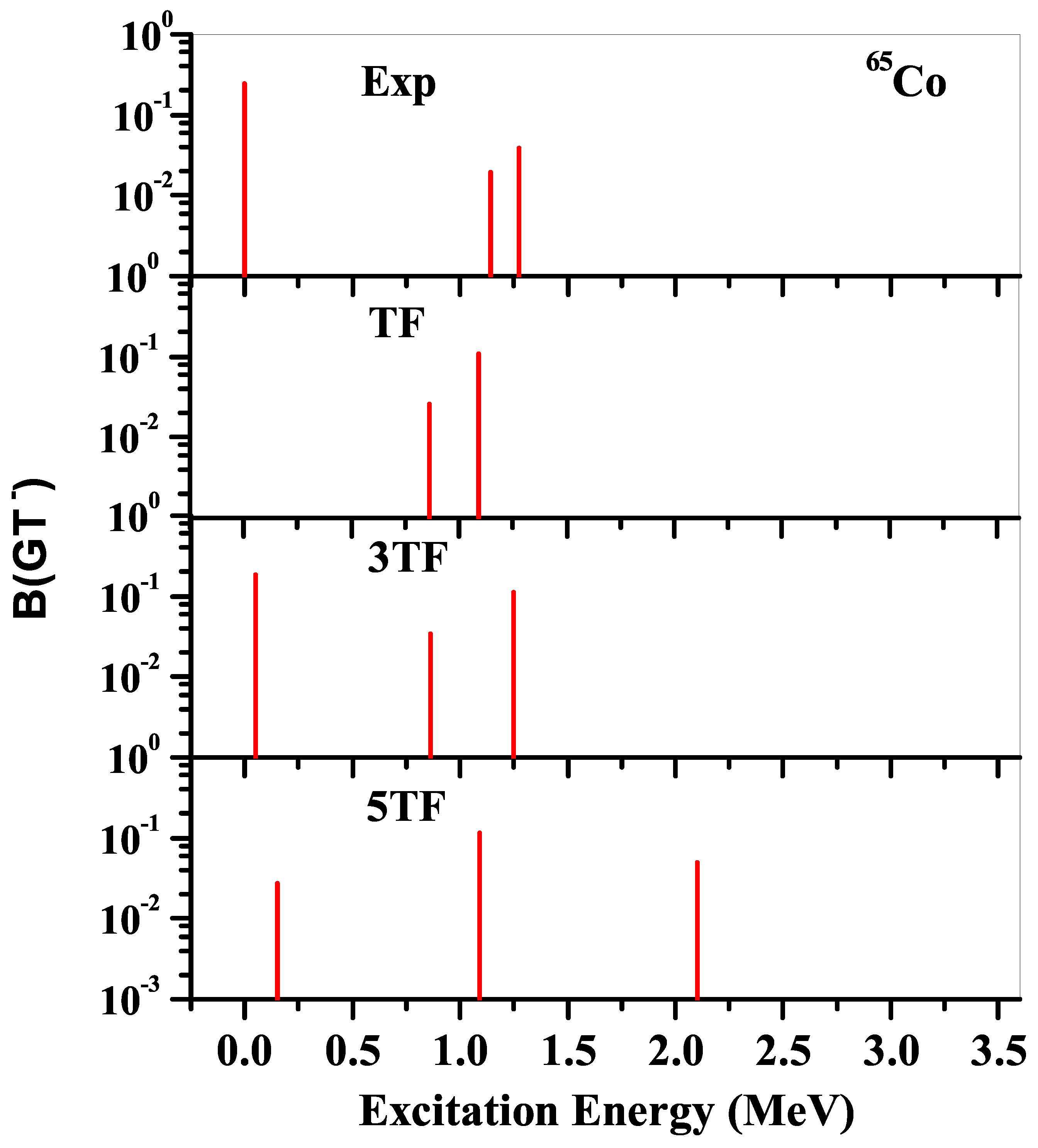
We first tested how well the different pairing gaps reproduced the measured GT distributions. For the needful comparison, we selected   63 Co with a β decay Q-value of 3.672 MeV and   65 Co with a β decay Q-value of 5.956 MeV. Figure 3 compares the calculated GT strength distributions with the experimental data [53,54]. All model parameters were kept fixed and were selected as stated in the previous section. The pairing gap parameters only varied. The 3TF pairing scheme resulted in a more fragmented distribution that compares well with the experimental data. Figure 4 shows a similar comparison for   65 Co. In this case, the measured data were taken from Refs. [54,55]. Here, the 5TF scheme resulted in a decent comparison but not better than the 3TF scheme. The conventional TF scheme resulted in a poor prediction of the GT spectra in both cases. The calculated GT distributions were in decent agreement with the measured data, validating the choice of the current nuclear model for the calculation of β -decay properties.
Branching ratios (I) of charge-changing transitions in the daughter were calculated using the following equation:
I = T 1 / 2 t ( 1 / 2 ) × 100 ( % ) .
Figure 5, Figure 6, Figure 7 and Figure 8 show the computed branching ratios and partial half-lives as functions of daughter excitation energy for the three selected pairing gaps (TF, 3TF, and 5TF) for   56 Mn,   67 Ni,   75 Ga, and   78 Ge, respectively. These nuclei were selected as belonging to odd–odd, even-odd, odd–even, and even–even categories from the top-ranked 50 nuclei for the analysis of branching ratios and partial half-lives. The fragmentation of the total GT strength (Figure 2) to low-lying states is altered by changing pairing gap values. The effect is different for different classes of nuclei. For odd–odd case, Figure 5 shows that low-lying transitions with more fragmentations are produced with 3TF and 5TF schemes. For the magic number nucleus   67 Ni, Figure 6 shows that the 5TF scheme results in considerable enhancement of the fragmentation of the GT strength when compared with the other two schemes. The 3TF and 5TF schemes resulted in similar GT distributions for the odd–even nucleus   75 Ga, as exhibited in Figure 7. Branching ratios less than 10−3 are not shown in these figures. For the even–even nucleus   78 Ge, Figure 8 reveals that the 3TF scheme resulted in one low-lying transition at 0.04 MeV (missing in the 5TF scheme) albeit with a small branching ratio. Equation (62) helps explain T 1 / 2 through t 1 / 2 . The middle and bottom panels of Figure 5 show that the t 1 / 2 of the β -decay of   56 Mn feeding the state with higher energy is comparable to the other two half-lives, but its branching ratio is almost four orders of magnitude smaller than the others. Likewise, in the bottom panel of Figure 6 ( 67 Ni ) , the state at energy, 0.31 MeV, has a very small branching ratio of 0.002 and, hence, the contribution of the partial half-life is negligible to the total computed half-life.
The comparison between calculated and measured half-lives for the selected top-ranked 50 nuclei is presented in Figure 9. The terrestrial half-lives were calculated using the pn-QRPA model with TF, 3TF, and 5TF pairing gap values. The calculated half-life depends on the total strength and distribution of the GT transitions in the daughter states. These two quantities were shown earlier in Figure 2 as functions of the pairing gaps. Three orders of magnitude or more differences in the calculated half-life values may be noted from Figure 9. Higher total GT strength values and lower placement of the GT centroid result in smaller calculated half-lives. Table 2 shows the accuracy of the current nuclear model using different pairing gap values as input parameters. We define the ratios of the calculated to measured half-lives using the variable y i , as follows:
y i = T 1 / 2 c a l T 1 / 2 e x p i f T 1 / 2 c a l T 1 / 2 e x p O R = T 1 / 2 e x p T 1 / 2 c a l i f T 1 / 2 c a l < T 1 / 2 e x p .
In Table 2, n is the number of half-lives (out of a total of 50 cases) reproduced under the condition given in the first column. The average deviation ( y ¯ ) was calculated using the following:
y = 1 n i = 1 n y i ,
Table 2 shows that the current model with the 3TF pairing gap reproduces 80 % ( 44 % ) of the measured half-life values within a factor of 10 (2), with an average deviation of 2.42 (1.22). We conclude that the 3TF pairing gap results in the calculation of a larger total GT strength and the best prediction of half-life values for the top-ranked 50 nuclei.
Because of the crucial importance of these nuclei in a stellar environment, we decided to calculate β -decay rates of the selected 50 nuclei as functions of pairing gaps in the stellar matter. For r-process nuclei under the prevailing physical conditions in stellar matter, forbidden transitions may also contribute to the total weak rates. In the current model, we only calculated the allowed GT and Fermi transitions. The calculation of weak rates, including forbidden transitions, will be looked at in a future assignment. In general, larger pairing gaps tend to shift the GT centroid to higher excitation energies in the daughter. This in turn decreases the β -decay rates. A larger pairing gap leads to a smaller number of nucleons occupying states near the Fermi level. This may result in a redistribution of the GT strength to higher excitation energies. Table 3, Table 4, Table 5, Table 6 and Table 7 show the β -decay rates of the top-ranked 50 nuclei at selected densities [ ρ Y e = (107, 109, 10 11 ) g cm−3], and temperatures [T = (5, 10, 15, 30) GK]. In these tables, entries written as <10−100 mean that the calculated β -decay rates are less than 10−100 s −1. At lower core densities, the abundance of these nuclei would almost be negligible. At high densities, the phase space is choked and β -decay rates tend to zero. Only at high core temperatures might the β -decay rates prove useful for collapse simulators. Table 3, Table 4, Table 5, Table 6 and Table 7 show that β -decay rates increase as the core temperature increases and decrease as ρ Y e increases. The decay rates, for a predetermined density, increase due to the accessibility of a large phase space with the increasing core temperature. Soaring core temperatures increase the occupation probabilities of parent-excited levels, thereby leading to a larger contribution of partial rates from parent-excited states to the total rates. As the stellar core becomes denser, the electron Fermi energy increases, leading to a substantial decrease in the β -decay rates at high stellar density values. It can be concluded from Table 3, Table 4, Table 5, Table 6 and Table 7 that the 3TF scheme leads to the calculation of the largest stellar β -decay rates. This has a direct correlation with the calculation of a larger total GT strength using the 3TF scheme. Table 8 shows the average values of the calculated stellar β -decay rates using different pairing gap values under predetermined physical conditions.

4. Conclusions and Summary

In this study, we re-examined the influence of pairing gaps on charge-changing transitions, partial half-lives, branching ratios, and weak rates for the top 50 astrophysically significant nuclei that are unstable to β decay. Pairing gaps are some of the most important model parameters in the pn-QRPA approach for the calculation of β -decay rates. In order to investigate the effect of pairing gaps on calculated GT strength distributions and half-lives, we used three different empirically calculated values (referred to as TF, 3TF, and 5TF). Changing pairing gap values led to significant alterations in the total GT strength and β -decay rates. It was concluded that the 3TF pairing gaps resulted in the best prediction of β -decay half-lives. The following main conclusions are drawn from the current investigation:
The available empirical formulae for pairing gaps give values of Δ p p differing by 0.5 MeV or more. The difference in Δ n n is more than 1 MeV.
The total GT strength and placement of the computed GT centroid change substantially with the pairing gap values. The 3TF pairing gap leads to lower placement of the GT centroid and higher total GT strength.
The 3TF scheme provides the best predictive power to the current pn-QRPA model.
The 3TF pairing gaps result in the largest stellar β -decay rates for the selected top-50 ranked nuclei.

Author Contributions

J.-U.N. and M.R. made significant contributions. A.M. assisted with operating servers and creating tables and figures. All authors have read and agreed to the published version of the manuscript.

Funding

This research ws funfed by the Higher Education Commission of Pakistan through project # 20-15394/NRPU/R&D/HEC/2021.

Institutional Review Board Statement

Not applicable.

Informed Consent Statement

Not applicable.

Data Availability Statement

No new data were created or analyzed in this study. Data sharing is not applicable to this article.

Conflicts of Interest

The authors declare no conflicts of interest.

Abbreviations

The following abbreviations are used:
pn-QRPAproton–neutron quasiparticle random-phase approximation
GTGamow–Teller
TFtraditional formula
3TF3-term formula
5TF5-term formula

References

  1. Bethe, H.A. Supernova mechanisms. Rev. Mod. Phys. 1990, 62, 801. [Google Scholar] [CrossRef]
  2. Langanke, K.; Martínez-Pinedo, G. Nuclear weak-interaction processes in stars. Rev. Mod. Phys. 2003, 75, 819. [Google Scholar] [CrossRef]
  3. Janka, H.T.; Langanke, K.; Marek, A.; Martínez-Pinedo, G.; Müller, B. Theory of core-collapse supernovae. Phys. Rep. 2007, 442, 38–74. [Google Scholar] [CrossRef]
  4. Bethe, H.A.; Brown, G.E.; Applegate, J.; Lattimer, J.M. Equation of state in the gravitational collapse of stars. Nucl. Phys. A 1979, 324, 487–533. [Google Scholar] [CrossRef]
  5. Hix, W.R.; Messer, O.E.B.; Mezzacappa, A.; Liebendörfer, M.; Sampaio, J.; Langanke, K.; Martínez-Pinedo, G. Consequences of nuclear electron capture in core collapse supernovae. Phys. Rev. Lett. 2003, 91, 201102. [Google Scholar] [CrossRef] [PubMed]
  6. Heger, A.; Woosley, S.E.; Martinez-Pinedo, G.; Langanke, K. Presupernova evolution with improved rates for weak interactions. Astrophys. J. 2001, 560, 307. [Google Scholar] [CrossRef]
  7. Martínez-Pinedo, G.; Lam, Y.H.; Langanke, K.; Zegers, R.G.T.; Sullivan, C. Astrophysical weak-interaction rates for selected A = 20 and A = 24 nuclei. Phys. Rev. C 2014, 89, 045806. [Google Scholar] [CrossRef]
  8. Suzuki, T.; Toki, H.; Nomoto, K.I. Electron-capture and β-decay rates for sd-shell nuclei in stellar environments relevant to high-density O–Ne–Mg cores. Astrophys. J. 2016, 817, 163. [Google Scholar] [CrossRef]
  9. Kirsebom, O.S.; Jones, S.; Strömberg, D.F.; Martínez-Pinedo, G.; Langanke, K.; Röpke, F.K.; Äystö, J. Discovery of an Exceptionally Strong β-Decay Transition of F 20 and Implications for the Fate of Intermediate-Mass Stars. Phys. Rev. Lett. 2019, 123, 262701. [Google Scholar] [CrossRef]
  10. Leung, S.C.; Fuller, J. Hydrodynamic Simulations of Pre-supernova Outbursts in Red Supergiants: Asphericity and Mass Loss. Astrophys. J. 2020, 900, 99. [Google Scholar] [CrossRef]
  11. Niu, Z.M.; Liang, H.Z. Nuclear mass predictions with machine learning reaching the accuracy required by r-process studies. Phys. Rev. C 2022, 106, L021303. [Google Scholar] [CrossRef]
  12. Burbidge, E.M.; Burbidge, G.R.; Fowler, W.A.; Hoyle, F. Synthesis of the elements in stars. Rev. Mod. Phys. 1957, 29, 547. [Google Scholar] [CrossRef]
  13. Smartt, S.; Chen, T.W.; Jerkstr, A.; Coughlin, M.; Kankare, E.; Sim, S.A.; Yaron, O. A kilonova as the electromagnetic counterpart to a gravitational-wave source. Nature 2017, 551, 75–79. [Google Scholar] [CrossRef] [PubMed]
  14. Watson, D.; Hansen, C.J.; Selsing, J.; Koch, A.; Malesani, D.B.; Andersen, A.C.; Pian, E. Identification of strontium in the merger of two neutron stars. Nature 2019, 574, 497–500. [Google Scholar] [CrossRef] [PubMed]
  15. Siegel, D.M.; Barnes, J.; Metzger, B.D. Collapsars as a major source of r-process elements. Nature 2019, 569, 241–244. [Google Scholar] [CrossRef] [PubMed]
  16. Borzov, I.N. Beta-decay rates. Nucl. Phys. A 2006, 777, 645–675. [Google Scholar] [CrossRef]
  17. Panov, I.V.; Lutostansky, Y.S.; Thielemann, F.K. Beta-decay half-lives for the r-process nuclei. Nucl. Phys. A 2016, 947, 1–11. [Google Scholar] [CrossRef]
  18. Takahashi, K.; Yamada, M.; Kondoh, T. β-decay half-lives calculated on the gross theory. At. Data Nucl. Data Tables 1973, 12, 101–142. [Google Scholar] [CrossRef]
  19. Nomura, K.; Rodríguez-Guzmán, R.; Robledo, L.M. β-decay of even-A nuclei within the interacting boson model with input based on nuclear density functional theory. Phys. Rev. C 2020, 101, 044318. [Google Scholar] [CrossRef]
  20. Engel, J.; Bender, M.; Dobaczewski, J.; Nazarewicz, W.; Surman, R. β-decay rates of r-process waiting-point nuclei in a self-consistent approach. Phys. Rev. C 1999, 60, 014302. [Google Scholar] [CrossRef]
  21. Kumar, A.; Srivastava, P.C.; Suzuki, T. Shell model results for nuclear β-decay properties of sd-shell nuclei. Prog. Theor. Exp. Phys. 2020, 3, 033D01. [Google Scholar] [CrossRef]
  22. Fuller, G.M.; Fowler, W.A.; Newman, M.J. Stellar weak-interaction rates for sd-shell nuclei. I-Nuclear matrix element systematics with application to Al-26 and selected nuclei of importance to the supernova problem. Astrophys. J. Suppl. Ser. 1980, 42, 447–473. [Google Scholar] [CrossRef]
  23. Dean, D.J.; Langanke, K.; Chatterjee, L.; Radha, P.B.; Strayer, M.R. Electron capture on iron group nuclei. Phys. Rev. C 1998, 58, 536. [Google Scholar] [CrossRef]
  24. Möller, P.; Randrup, J. New developments in the calculation of β-strength functions. Nucl. Phys. A 1990, 514, 1–48. [Google Scholar] [CrossRef]
  25. Nabi, J.-U.; Klapdor-Kleingrothaus, H.V. Weak interaction rates of sd-shell nuclei in stellar environments calculated in the proton-neutron quasiparticle random-phase approximation. At. Data Nucl. Data Tables 1999, 71, 149. [Google Scholar] [CrossRef]
  26. Nabi, J.-U.; Klapdor-Kleingrothaus, H.V. Microscopic calculations of stellar weak interaction rates and energy losses for fp-and fpg-shell nuclei. At. Data Nucl. Data Tables 2004, 88, 237–476. [Google Scholar] [CrossRef]
  27. Nabi, J.-U.; Riaz, M.; Bayram, T.; Azaz, M. Effect of Nuclear Deformation on Gamow teller Strength Distributions of Hg Isotopes. Braz. J. Phys. 2022, 52, 161. [Google Scholar] [CrossRef]
  28. Ullah, A.; Nabi, J.-U. Stellar Weak Rates and Mass Fractions of 20 Most Important fp-shell Nuclei with A < 65. Braz. J. Phys. 2022, 52, 13. [Google Scholar]
  29. Ullah, A.; Nabi, J.-U.; Tahir, M. Investigation of effects of pairing correlations on calculated β-decay half-lives of fp-shell nuclei. Braz. J. Phys. 2023, 53, 39. [Google Scholar] [CrossRef]
  30. Nabi, J.-U.; Ullah, A.; Khan, A.A. Investigation of important weak interaction nuclei in presupernova evolution. Astrophys. J. 2021, 911, 93. [Google Scholar] [CrossRef]
  31. Kondev, F.G.; Wang, M.; Huang, W.J.; Naimi, S.; Audi, G. The NUBASE2020 evaluation of nuclear physics properties. Chin. Phys. C. 2021, 45, 030001. [Google Scholar] [CrossRef]
  32. Ha, E.; Cheoun, M.-K.; Sagawa, H. Tensor force effect on pairing correlation for the Gamow-Teller transitions in 42Ca, 46Ti, and 10O. Prog. Theor. Exp. Phys. 2022, 043, D01. [Google Scholar]
  33. Hirsch, M.; Staudt, A.; Muto, K.; Klapdor-Kleingrothaus, H.V. Microscopic predictions of β+/EC-decay half-lives. At. Data Nucl. Data Tables 1993, 53, 165–193. [Google Scholar] [CrossRef]
  34. Jensen, A.S.; Hansen, P.G.; Jonson, B. New mass relations and two-and four-nucleon correlations. Nucl. Phys. A. 1984, 431, 393–418. [Google Scholar] [CrossRef]
  35. Satuła, W.; Dobaczewski, J.; Nazarewicz, W. Odd-even staggering of nuclear masses: Pairing or shape effect. Phys. Rev. Lett. 1998, 81, 3599. [Google Scholar] [CrossRef]
  36. Bender, M.; Rutz, K.; Reinhard, P.G.; Maruhn, J.A. Pairing gaps from nuclear mean-field models. Eur. Phys. J. A 2000, 8, 59–75. [Google Scholar] [CrossRef]
  37. Magner, A.G.; Sanzhur, A.I.; Fedotkin, S.N.; Levon, A.I.; Grygoriev, U.V.; Shlomo, S. Paring correlations within the micro-macroscopic approach for the level density. Eur. Phys. J. A 2023, 2308, 07784. [Google Scholar]
  38. Lindhard, J.; Scharff, M. Binding states of individual nucleons in strongly deformed nuclei. Mat. Fys. Medd. Dan. Vid. Selsk. 1955, 28, 1–68. [Google Scholar]
  39. Möller, P.; Sierk, A.J.; Ichikawa, T.; Sagawa, H. Nuclear ground-state masses and deformations: FRDM (2012). At. Data Nucl. Data Tables 2016, 109, 1–204. [Google Scholar] [CrossRef]
  40. Ragnarsson, I.; Sheline, R.K. Systematic of nuclear deformations. Phys. Scr. 1984, 29, 385. [Google Scholar] [CrossRef]
  41. Staudt, A.; Bender, E.; Muto, K.; Klapdor-Kleingrothaus, H.V. Second-generation microscopic predictions of beta-decay half-lives of neutron-rich nuclei. At. Data Nucl. Data Tables 1990, 44, 79–132. [Google Scholar] [CrossRef]
  42. Homma, H.; Bender, E.; Hirsch, M.; Muto, K.; Klapdor-Kleingrothaus, H.V.; Oda, T. Systematic study of nuclear β decay. Phys. Rev. C 1996, 54, 2972. [Google Scholar] [CrossRef] [PubMed]
  43. Wang, M.; Huang, W.J.; Kondev, F.G.; Audi, G.; Naimi, S. The AME 2020 atomic mass evaluation (II). Tables, graphs and references. Chin. Phys. C 2021, 45, 030003. [Google Scholar] [CrossRef]
  44. Muto, K.; Bender, E.; Oda, T.; Klapdor-Kleingrothaus, H.V. Proton-neutron quasiparticle RPA with separable Gamow-Teller forces. Z. Phys. A Hadron. Nucl. 1992, 341, 407–415. [Google Scholar] [CrossRef]
  45. Muto, K.; Bender, E.; Klapdor-Kleingrothaus, H.V. Effects of ground-state correlations on 2νββ decay rates and limitations of the QRPA approach. Z. Phys. A Atom. Nucl. 1989, 334, 177–186. [Google Scholar] [CrossRef]
  46. Hardy, J.C.; Towner, I.S. Superallowed 0+→0+ nuclear β decays: A new survey with precision tests of the conserved vector current hypothesis and the standard model. Phys. Rev. C 2009, 79, 055502. [Google Scholar] [CrossRef]
  47. Nakamura, K. Particle Data Group. J. Phys. G Nucl. Part. Phys. 2010, 37, 075021. [Google Scholar] [CrossRef]
  48. Towner, I.S. Quenching of spin matrix elements in nuclei. Phys. Rep. 1987, 155, 263–377. [Google Scholar] [CrossRef]
  49. Gysbers, P.; Hagen, G.; Holt, J.D.; Jansen, G.R.; Morris, T.D.; Navratil, P.; Papenbrock, T.; Quaglioni, S.; Schwenk, A.; Stroberg, S.R.; et al. Discrepancy between experimental and theoretical β-decay rates resolved from first principles. Nat. Phys. 2019, 15, 428. [Google Scholar] [CrossRef]
  50. Hirsch, M.; Staudt, A.; Muto, K.; Klapdor-Kleingrothaus, H.V. Microscopic calculation of β+ EC decay half-lives with atomic number Z = 10–30. Nucl. Phys. A 1991, 535, 62–76. [Google Scholar] [CrossRef]
  51. Gove, N.B.; Martin, M.J. LOG-f Tables for Beta Decay. At. Data Nucl. Data Tables 1971, 10, 205. [Google Scholar] [CrossRef]
  52. Ikeda, K. Collective Excitation of Unlike Pair States in Heavier Nuclei. Prog. Theor. Phys. 1964, 31, 434–451. [Google Scholar] [CrossRef]
  53. Jongsma, H.W.; Kamermans, R.; Verheul, H. The decay of 63Co. Z. Phys. 1972, 251, 425–430. [Google Scholar] [CrossRef]
  54. Runte, E.; Gippert, K.L.; Schmidt-Ott, W.D.; Tidemand-Petersson, P.; Ziegeler, L.; Kirchner, R.; Klepper, O.; Larsson, P.O.; Roeckl, E.; Schardt, D.; et al. Decay studies of neutron-rich isotopes of manganese, iron, cobalt, nickel, copper and zinc. Nuc. Phys. A 1985, 441, 237–260. [Google Scholar] [CrossRef]
  55. Pauwels, D.; Ivanov, O.; Bree, N.; Büscher, J.; Cocolios, T.E.; Huyse, M.; Kudryavtsev, Y.; Raabe, R.; Sawicka, M.; Van de Walle, J.; et al. Structure of 65,67Co studied through the β-decay of 65,67Fe and a deep-inelastic reaction. Phys. Rev. C 1972, 79, 044309. [Google Scholar] [CrossRef]
Figure 1. Computed pairing gap values of the selected 50 nuclei used in the current investigation.
Universe 10 00128 g001
Figure 2. The total strength and centroid values of the calculated GT distributions of the selected 50 nuclei.
Universe 10 00128 g002
Figure 3. Comparison between measured and calculated GT distributions of   63 Co. Experimental data were taken from Refs. [53,54].
Universe 10 00128 g003
Figure 4. Comparison between measured and calculated GT distributions of   65 Co. Experimental data were taken from Refs. [54,55].
Universe 10 00128 g004
Figure 5. Calculated branching ratios (I) and partial half-lives ( t 1 / 2 ) for the β -decay of   56 Mn as functions of the pairing gaps within the Q-value window. E j shows the excited energy in the daughter nucleus.
Universe 10 00128 g005
Figure 6. Calculated branching ratios (I) and partial half-lives ( t 1 / 2 ) for the β -decay of   67 Ni as functions of pairing gaps within the Q-value window. E j shows excited energy in the daughter nucleus.
Universe 10 00128 g006
Figure 7. Calculated branching ratios (I) and partial half-lives ( t 1 / 2 ) for the β -decay of   75 Ga as functions of pairing gaps within the Q-value window. E j shows excited energy in the daughter nucleus.
Universe 10 00128 g007
Figure 8. Calculated branching ratios (I) and partial half-lives ( t 1 / 2 ) for the β -decay of   78 Ge as functions of pairing gaps within the Q-value window. E j shows excited energy in the daughter nucleus.
Universe 10 00128 g008
Figure 9. Comparison between measured and predicted half-lives using three different pairing gap values for the selected nuclei. Measured half-lives were taken from Ref. [31].
Universe 10 00128 g009
Table 1. The uncertainty associated with the computation of pairing gap values for the selected nuclei.
Nuclei Δ pp 3 TF σ pp 3 TF Δ nn 3 TF σ nn 3 TF Δ pp 5 TF σ pp 5 TF Δ nn 5 TF σ nn 5 TF
  56 Mn1.2199(±0.01262)1.0826(±0.0110)1.2442(±0.0001)0.9924(±0.0002)
  52 V1.4051(±0.0025)1.2272(±0.0031)1.4160(±0.0002)1.0549(±0.0001)
  67 Cu1.7205(±0.0020)1.2201(±0.0015)1.4529(±0.0001)1.2019(±0.0001)
  67 Ni1.9130(±0.0139)1.2822(±0.0029)1.7737(±0.0001)1.2899(±0.0002)
  60 Co1.3590(±0.0021)1.1972(±0.0011)1.3787(±0.0002)1.1672(±0.0001)
  49 Sc2.1768(±0.0022)1.4937(±0.0049)1.9171(±0.0001)1.3496(±0.0001)
  66 Cu1.1727(±0.02000)1.2278(±0.0008)0.9495(±0.0001)1.2239(±0.0003)
  50 Sc1.9343(±0.0025)1.2055(±0.0049)1.6477(±0.0001)0.8751(±0.0001)
  79 Ge1.0129(±0.0371)1.3296(±0.0371)1.0833(±0.0004)1.3652(±0.0004)
  65 Co1.6184(±0.0050)0.9056(±0.0200)1.8231(±0.0003)0.9350(±0.0001)
  63 Co1.6088(±0.0185)1.0975(±0.0200)1.7241(±0.0003)1.0406(±0.0002)
  77 Ga1.5809(±0.0035)0.9609(±0.0024)1.5749(±0.0001)0.8700(±0.0001)
  78 Ge1.5680(±0.0053)1.4075(±0.0371)1.5901(±0.0004)1.3700(±0.0001)
  83 As1.3892(±0.0032)1.3430(±0.0037)1.4039(±0.0001)1.2378(±0.0001)
  51 Ti1.3611(±0.0025)1.5025(±0.0027)1.3831(±0.0001)1.2243(±0.0001)
  59 Mn1.5931(±0.0847)0.9028(±0.0027)1.6418(±0.0001)0.8997(±0.0014)
  64 Co1.0334(±0.0200)0.9853(±0.0200)1.1886(±0.0003)0.9449(±0.0003)
  49 Ca1.9691(±0.0025)1.5047(±0.0022)1.9517(±0.0001)1.0974(±0.0001)
  58 Cr1.6375(±0.1002)1.3923(±0.0029)1.6181(±0.0001)1.4475(±0.0017)
  68 Cu1.6340(±0.0139)1.1839(±0.0015)1.2401(±0.0001)1.1982(±0.0002)
  82 As1.1693(±0.0037)1.1848(±0.0037)1.1112(±0.0001)1.2637(±0.0001)
  75 Ga1.5284(±0.0025)1.1589(±0.0029)1.5263(±0.0001)1.1338(±0.0001)
  69 Cu1.8563(±0.0064)1.2126(±0.0015)1.5295(±0.0001)1.2842(±0.0001)
  57 Ni1.4860(±0.0005)2.0909(±0.0007)1.2959(±0.0001)1.6936(±0.0001)
  61 Fe1.1374(±0.0185)1.4226(±0.0034)1.1978(±0.0001)1.4176(±0.0002)
  81 Ge1.1328(±0.0037)1.4039(±0.0371)1.1508(±0.0004)1.4434(±0.0001)
  78 Ga0.9509(±0.0371)0.7791(±0.0024)0.9806(±0.0001)0.8022(±0.0004)
  51 Sc2.2206(±0.0027)0.5445(±0.0030)1.9128(±0.0003)0.5739(±0.0001)
  64 Cu1.1883(±0.0185)1.2356(±0.0006)1.0006(±0.0001)1.2227(±0.0002)
  57 Cr1.2598(±0.1758)1.2904(±0.0029)1.2004(±0.0001)1.3414(±0.0031)
  77 Ge1.1226(±0.0097)1.5012(±0.0035)1.1623(±0.0004)1.4548(±0.0001)
  55 Cr1.4016(±0.0111)1.3681(±0.0005)1.3107(±0.0001)1.3009(±0.0002)
  83 Se1.0541(±0.0257)1.5793(±0.0030)1.0326(±0.0001)1.6650(±0.0003)
  62 Fe1.6161(±0.0185)1.4124(±0.0043)1.6126(±0.0001)1.4283(±0.0002)
  48 Sc1.6681(±0.00495)1.0748(±0.004)1.4966(±0.0001)1.2842(±0.0001)
  65 Ni1.3447(±0.02000)1.6032(±0.0013)1.2584(±0.0001)1.5513(±0.0003)
  57 Mn1.6066(±0.0270)0.9021(±0.0027)1.6861(±0.0001)0.8998(±0.0004)
  71 Cu1.8159(±0.0856)1.2893(±0.0014)1.6357(±0.0001)1.2441(±0.0012)
  53 Ti1.3766(±0.0111)0.9499(±0.0158)1.3804(±0.0005)1.0040(±0.0002)
  53 V1.6405(±0.0031)0.8829(±0.0118)1.6974(±0.0004)0.8841(±0.0001)
  73 Ga1.5124(±0.0021)1.3556(±0.0029)1.5412(±0.0001)1.2805(±0.0001)
  85 Br1.4286(±0.0030)1.4394(±0.02573)1.3917(±0.0003)1.3371(±0.0001)
  62 Co1.2586(±0.0185)1.1560(±0.0185)1.3493(±0.0003)1.1262(±0.0002)
  70 Cu1.6734(±0.0038)1.3558(±0.0015)1.3925(±0.0001)1.3226(±0.0001)
  76 Ga0.9984(±0.0061)1.1087(±0.0029)1.0605(±0.0001)1.0347(±0.0001)
  73 Zn1.1969(±0.0029)1.5210(±0.0026)1.1866(±0.0001)1.5200(±0.0001)
  80 Ge1.4776(±0.00264)1.3965(±0.0371)1.4952(±0.0004)1.4016(±0.0001)
  63 Ni1.4407(±0.0185)1.6443(±0.0004)1.3143(±0.0001)1.6195(±0.0002)
  67 Co1.6837(±0.0064)1.0702(±0.0139)1.9365(±0.0012)1.1621(±0.0001)
  61 Co1.6913(±0.0034)1.1372(±0.0185)1.7680(±0.0002)1.1463(±0.0001)
  63 Fe1.0101(±0.0200)1.4439(±0.0050)1.0213(±0.0001)1.4297(±0.0003)
Table 2. Accuracy of the pn-QRPA model calculated the half-lives using three different pairing gaps for the selected 50 top-ranked β -decaying nuclei.
ConditionPairing Gapsnn% y ¯
y i ≤ 10TF39782.81
3TF40802.42
5TF36723.18
y i ≤ 2TF21421.32
3TF22441.22
5TF18361.42
Table 3. Comparison of calculated stellar β -decay rates for 48–51Sc,   49 Ca,   51 , 53 Ti,   52 , 53 V,   55 Cr, and   56 Mn as functions of pairing gap values. The stellar core temperatures are given in units of G K , and densities are given in units of gcm−3.
NucleiT ρ = 10 7 ρ = 10 9 ρ = 10 11
TF3TF5TFTF3TF5TFTF3TF5TF
  48 Sc59.16 × 10 05 1.00 × 10 03 4.51 × 10 04 2.06 × 10 07 1.60 × 10 06 8.75 × 10 07 8.02 × 10 26 1.42 × 10 24 4.13 × 10 25
 105.45 × 10 03 1.10 × 10 02 1.01 × 10 02 5.33 × 10 04 1.24 × 10 03 1.24 × 10 03 2.59 × 10 13 1.00 × 10 12 6.55 × 10 13
 153.49 × 10 02 7.36 × 10 02 7.18 × 10 02 9.86 × 10 03 2.32 × 10 02 2.25 × 10 02 5.26 × 10 09 1.54 × 10 08 1.24 × 10 08
 302.43 × 10 01 6.10 × 10 01 5.73 × 10 01 1.87 × 10 01 4.76 × 10 01 4.46 × 10 01 1.44 × 10 04 3.91 × 10 04 3.50 × 10 04
  49 Ca55.62 × 10 02 3.46 × 10 02 2.17 × 10 02 4.04 × 10 03 2.54 × 10 03 2.20 × 10 03 5.47 × 10 21 4.04 × 10 21 4.07 × 10 21
 103.80 × 10 01 2.52 × 10 01 2.40 × 10 01 1.25 × 10 01 8.45 × 10 02 8.59 × 10 02 1.14 × 10 10 9.12 × 10 11 8.73 × 10 11
 151.25 × 10 + 00 9.93 × 10 01 9.64 × 10 01 6.11 × 10 01 4.95 × 10 01 4.86 × 10 01 5.36 × 10 07 6.79 × 10 07 4.58 × 10 07
 306.12 × 10 + 00 1.22 × 10 + 01 5.48 × 10 + 00 5.07 × 10 + 00 1.04 × 10 + 01 4.56 × 10 + 00 5.45 × 10 03 1.75 × 10 02 5.13 × 10 03
  49 Sc57.71 × 10 04 1.21 × 10 03 9.08 × 10 04 1.23 × 10 06 1.99 × 10 06 1.40 × 10 06 3.33 × 10 24 2.94 × 10 24 2.78 × 10 24
 105.14 × 10 03 5.43 × 10 03 5.09 × 10 03 7.31 × 10 04 6.31 × 10 04 6.53 × 10 04 1.25 × 10 12 1.11 × 10 12 1.01 × 10 12
 155.28 × 10 02 3.85 × 10 02 4.03 × 10 02 1.86 × 10 02 1.37 × 10 02 1.32 × 10 02 1.63 × 10 08 1.60 × 10 08 1.15 × 10 08
 306.79 × 10 01 1.04 × 10 + 00 4.28 × 10 01 5.33 × 10 01 8.49 × 10 01 3.31 × 10 01 4.56 × 10 04 9.98 × 10 04 2.70 × 10 04
  50 Sc57.52 × 10 03 8.20 × 10 03 9.77 × 10 03 1.37 × 10 04 1.02 × 10 04 2.25 × 10 04 3.06 × 10 23 7.11 × 10 23 8.28 × 10 23
 101.04 × 10 01 9.16 × 10 02 1.24 × 10 01 1.66 × 10 02 1.32 × 10 02 2.25 × 10 02 7.89 × 10 12 1.13 × 10 11 1.28 × 10 11
 153.58 × 10 01 3.44 × 10 01 5.09 × 10 01 1.24 × 10 01 1.18 × 10 01 1.88 × 10 01 7.21 × 10 08 9.40 × 10 08 1.17 × 10 07
 301.79 × 10 + 00 1.92 × 10 + 00 3.03 × 10 + 00 1.41 × 10 + 00 1.52 × 10 + 00 2.42 × 10 + 00 1.19 × 10 03 1.38 × 10 03 2.08 × 10 03
  51 Sc53.04 × 10 02 1.15 × 10 02 1.04 × 10 02 2.14 × 10 03 7.71 × 10 04 6.81 × 10 04 4.68 × 10 20 3.70 × 10 20 3.47 × 10 20
 101.58 × 10 01 9.59 × 10 02 1.28 × 10 01 4.73 × 10 02 1.68 × 10 02 2.46 × 10 02 1.28 × 10 10 7.48 × 10 11 6.79 × 10 11
 151.05 × 10 + 00 4.01 × 10 01 5.68 × 10 01 5.22 × 10 01 1.45 × 10 01 2.11 × 10 01 6.22 × 10 07 2.37 × 10 07 2.10 × 10 07
 308.61 × 10 + 00 3.13 × 10 + 00 2.79 × 10 + 00 7.16 × 10 + 00 2.55 × 10 + 00 2.22 × 10 + 00 8.15 × 10 03 3.33 × 10 03 2.06 × 10 03
  51 Ti54.62 × 10 03 3.56 × 10 03 2.86 × 10 03 8.87 × 10 05 7.98 × 10 05 7.83 × 10 05 1.48 × 10 23 1.35 × 10 23 1.44 × 10 23
 104.63 × 10 02 4.41 × 10 02 4.32 × 10 02 7.67 × 10 03 7.60 × 10 03 7.87 × 10 03 2.86 × 10 12 2.91 × 10 12 3.10 × 10 12
 151.63 × 10 01 1.86 × 10 01 1.80 × 10 01 5.69 × 10 02 6.71 × 10 02 6.58 × 10 02 2.80 × 10 08 3.53 × 10 08 3.41 × 10 08
 308.73 × 10 02 1.95 × 10 + 00 1.03 × 10 + 00 6.89 × 10 01 1.56 × 10 + 00 8.17 × 10 01 5.53 × 10 04 1.37 × 10 03 6.81 × 10 04
  52 V55.41 × 10 04 8.32 × 10 04 7.38 × 10 04 1.46 × 10 06 4.92 × 10 06 4.40 × 10 06 1.61 × 10 25 5.85 × 10 25 5.22 × 10 25
 101.34 × 10 02 1.98 × 10 02 1.91 × 10 02 1.01 × 10 03 2.02 × 10 03 1.97 × 10 03 2.90 × 10 13 6.27 × 10 13 6.08 × 10 13
 155.19 × 10 02 8.61 × 10 02 8.81 × 10 02 1.27 × 10 02 2.43 × 10 02 2.49 × 10 02 4.95 × 10 09 1.01 × 10 08 1.04 × 10 08
 302.81 × 10 01 5.27 × 10 01 5.69 × 10 01 2.11 × 10 01 4.04 × 10 01 4.36 × 10 01 1.41 × 10 04 2.86 × 10 04 3.08 × 10 04
  53 Ti54.70 × 10 02 2.71 × 10 02 2.82 × 10 02 9.77 × 10 03 5.81 × 10 03 6.04 × 10 03 1.16 × 10 20 9.35 × 10 21 9.53 × 10 21
 105.36 × 10 01 4.28 × 10 01 4.36 × 10 01 1.82 × 10 01 1.54 × 10 01 1.56 × 10 01 1.52 × 10 10 1.61 × 10 10 1.60 × 10 10
 151.54 × 10 + 00 1.63 × 10 + 00 1.59 × 10 + 00 7.48 × 10 01 8.28 × 10 01 8.04 × 10 01 6.32 × 10 07 8.59 × 10 7 8.00 × 10 07
 306.32 × 10 + 00 1.18 × 10 + 01 7.50 × 10 + 00 5.24 × 10 + 00 9.89 × 10 + 00 6.25 × 10 + 00 5.61 × 10 03 1.22 × 10 02 7.28 × 10 03
  53 V55.93 × 10 03 3.72 × 10 03 4.24 × 10 03 2.43 × 10 05 1.71 × 10 05 1.70 × 10 05 2.18 × 10 23 1.40 × 10 23 1.14 × 10 23
 102.78 × 10 02 1.85 × 10 02 2.02 × 10 02 4.63 × 10 03 2.29 × 10 03 2.30 × 10 03 2.98 × 10 12 1.39 × 10 12 1.25 × 10 12
 152.17 × 10 01 1.10 × 10 01 1.14 × 10 01 7.89 × 10 02 3.40 × 10 02 3.37 × 10 02 4.66 × 10 08 1.86 × 10 08 1.70 × 10 08
 301.82 × 10 + 00 1.07 × 10 + 00 6.97 × 10 01 1.44 × 10 + 00 8.36 × 10 01 5.38 × 10 01 1.21 × 10 03 6.93 × 10 04 4.05 × 10 04
  55 Cr59.64 × 10 03 7.23 × 10 03 6.82 × 10 03 9.10 × 10 05 6.53 × 10 05 6.12 × 10 05 1.29 × 10 23 9.25 × 10 24 8.47 × 10 24
 104.47 × 10 02 3.21 × 10 02 3.13 × 10 02 5.79 × 10 03 4.17 × 10 03 4.00 × 10 03 2.03 × 10 12 1.49 × 10 12 1.37 × 10 12
 151.22 × 10 01 1.02 × 10 01 9.48 × 10 02 3.87 × 10 02 3.31 × 10 02 3.01 × 10 02 1.83 × 10 08 1.73 × 10 08 1.39 × 10 08
 305.41 × 10 01 1.00 × 10 + 00 4.56 × 10 01 4.22 × 10 01 8.00 × 10 01 3.56 × 10 01 3.27 × 10 04 7.41 × 10 04 2.74 × 10 04
  56 Mn51.57 × 10 04 5.77 × 10 04 5.05 × 10 04 1.40 × 10 07 7.23 × 10 07 5.82 × 10 07 1.76 × 10 26 9.23 × 10 26 7.71 × 10 26
 102.81 × 10 03 5.97 × 10 03 5.60 × 10 03 1.56 × 10 04 3.93 × 10 04 3.66 × 10 04 5.01 × 10 04 1.31 × 10 13 1.24 × 10 13
 151.14 × 10 02 2.45 × 10 02 2.41 × 10 02 2.54 × 10 03 5.87 × 10 03 5.78 × 10 03 1.04 × 10 09 2.48 × 10 09 2.45 × 10 09
 307.05 × 10 02 1.60 × 10 01 1.63 × 10 01 5.25 × 10 02 1.20 × 10 01 1.23 × 10 01 3.47 × 10 05 8.15 × 10 05 8.36 × 10 05
Table 4. Comparison of calculated stellar β -decay rates for   57 , 58 Cr,   57 , 59 Mn,   57 Ni, 60–63Co, and 61–63Fe as functions of pairing gap values. The stellar core temperatures are given in units of G K and densities are given in units of gcm−3.
NucleiT ρ = 10 7 ρ = 10 9 ρ = 10 11
TF3TF5TFTF3TF5TFTF3TF5TF
  57 Cr51.31 × 10 02 1.17 × 10 01 1.16 × 10 01 1.68 × 10 03 7.64 × 10 03 7.64 × 10 03 1.46 × 10 20 2.59 × 10 21 2.67 × 10 21
 101.34 × 10 01 3.23 × 10 01 3.24 × 10 01 4.75 × 10 02 7.38 × 10 02 7.43 × 10 02 2.04 × 10 010 4.03 × 10 11 4.09 × 10 11
 156.84 × 10 01 8.87 × 10 01 8.55 × 10 01 3.69 × 10 01 3.61 × 10 01 3.46 × 10 01 8.39 × 10 07 2.40 × 10 07 2.21 × 10 07
 304.63 × 10 + 00 5.43 × 10 + 00 3.44 × 10 + 00 3.94 × 10 + 00 4.43 × 10 + 00 2.77 × 10 + 00 6.05 × 10 03 4.50 × 10 03 2.55 × 10 03
  57 Mn58.81 × 10 03 8.32 × 10 03 8.32 × 10 03 1.51 × 10 05 1.36 × 10 05 1.36 × 10 05 3.46 × 10 24 2.13 × 10 24 2.66 × 10 24
 101.59 × 10 02 1.31 × 10 02 1.31 × 10 02 1.27 × 10 03 7.80 × 10 04 8.09 × 10 04 5.85 × 10 13 3.22 × 10 13 3.72 × 10 13
 156.21 × 10 02 3.54 × 10 02 3.26 × 10 02 1.70 × 10 02 8.71 × 10 03 7.60 × 10 03 8.28 × 10 09 5.64 × 10 09 3.81 × 10 09
 304.31 × 10 01 4.30 × 10 01 1.46 × 10 01 3.30 × 10 01 3.44 × 10 01 1.10 × 10 01 2.42 × 10 04 4.06 × 10 04 7.83 × 10 05
  57 Ni5 < 10 100 3.21 × 10 20 < 10 100 < 10 100 2.47 × 10 24 < 10 100 < 10 100 2.49 × 10 43 < 10 100
 10 < 10 100 1.79 × 10 13 < 10 100 < 10 100 2.55 × 10 15 < 10 100 < 10 100 5.90 × 10 25 < 10 100
 15 < 10 100 2.86 × 10 11 < 10 100 < 10 100 2.99 × 10 12 < 10 100 < 10 100 8.45 × 10 19 < 10 100
 30 < 10 100 5.14 × 10 09 < 10 100 < 10 100 3.44 × 10 09 < 10 100 < 10 100 1.60 × 10 12 < 10 100
  58 Cr56.82 × 10 02 7.29 × 10 02 7.18 × 10 02 1.40 × 10 03 1.49 × 10 03 1.54 × 10 03 3.23 × 10 21 2.96 × 10 21 2.99 × 10 21
 105.06 × 10 01 5.89 × 10 01 5.26 × 10 01 1.71 × 10 01 1.94 × 10 01 1.73 × 10 01 2.13 × 10 10 2.26 × 10 10 1.95 × 10 10
 151.50 × 10 + 00 2.47 × 10 + 00 1.45 × 10 + 00 7.60 × 10 01 1.23 × 10 + 00 7.19 × 10 01 8.32 × 10 07 1.31 × 10 06 7.31 × 10 07
 302.27 × 10 + 00 8.20 × 10 + 00 2.06 × 10 + 00 1.90 × 10 + 00 6.87 × 10 + 00 1.71 × 10 + 00 2.30 × 10 03 8.71 × 10 03 1.99 × 10 03
  59 Mn52.45 × 10 01 2.54 × 10 01 2.52 × 10 01 1.29 × 10 02 1.42 × 10 02 1.40 × 10 02 2.99 × 10 21 3.42 × 10 21 3.14 × 10 21
 103.43 × 10 01 4.06 × 10 01 4.12 × 10 01 6.43 × 10 02 7.26 × 10 02 7.35 × 10 02 3.32 × 10 11 3.77 × 10 11 3.48 × 10 11
 159.02 × 10 01 8.99 × 10 01 9.40 × 10 01 3.40 × 10 01 3.19 × 10 01 3.30 × 10 01 2.12 × 10 07 2.08 × 10 07 1.90 × 10 07
 304.27 × 10 + 00 4.02 × 10 + 00 3.16 × 10 + 00 3.41 × 10 + 00 3.21 × 10 + 00 2.49 × 10 + 00 3.08 × 10 03 3.18 × 10 03 2.13 × 10 03
  60 Co53.61 × 10 05 1.32 × 10 04 1.31 × 10 04 2.12 × 10 08 7.11 × 10 08 7.08 × 10 08 2.81 × 10 27 8.97 × 10 27 9.16 × 10 27
 107.67 × 10 04 1.67 × 10 03 1.60 × 10 03 4.34 × 10 05 8.24 × 10 05 8.17 × 10 05 1.35 × 10 14 2.43 × 10 14 2.44 × 10 14
 153.56 × 10 03 6.73 × 10 03 6.59 × 10 03 8.02 × 10 04 1.42 × 10 03 1.40 × 10 03 3.21 × 10 10 5.38 × 10 10 5.33 × 10 10
 302.28 × 10 02 4.03 × 10 02 3.90 × 10 02 1.69 × 10 02 2.97 × 10 02 2.88 × 10 02 1.10 × 10 05 1.87 × 10 05 1.81 × 10 05
  61 Co58.59 × 10 04 5.04 × 10 + 00 7.23 × 10 04 5.77 × 10 07 1.40 × 10 + 00 4.36 × 10 07 6.61 × 10 26 3.48 × 10 15 5.50 × 10 26
 103.27 × 10 03 8.65 × 10 + 00 2.51 × 10 03 1.81 × 10 04 4.04 × 10 + 00 1.37 × 10 04 5.32 × 10 14 5.79 × 10 08 4.26 × 10 14
 151.37 × 10 02 2.37 × 10 + 01 9.64 × 10 03 3.10 × 10 03 1.49 × 10 + 01 2.21 × 10 03 1.21 × 10 02 5.89 × 10 05 8.85 × 10 10
 309.55 × 10 02 1.26 × 10 + 02 6.47 × 10 02 7.18 × 10 02 1.10 × 10 + 02 4.88 × 10 02 4.82 × 10 05 2.23 × 10 01 3.30 × 10 05
  61 Fe55.36 × 10 02 4.52 × 10 02 4.69 × 10 02 1.66 × 10 03 1.50 × 10 03 1.53 × 10 03 3.43 × 10 22 2.73 × 10 22 2.74 × 10 22
 101.53 × 10 01 1.37 × 10 01 1.41 × 10 01 2.57 × 10 02 2.19 × 10 02 2.25 × 10 02 1.12 × 10 11 8.81 × 10 12 8.97 × 10 12
 154.53 × 10 01 4.01 × 10 01 4.02 × 10 01 1.60 × 10 01 1.38 × 10 01 1.38 × 10 01 8.89 × 10 08 7.52 × 10 08 7.18 × 10 08
 302.18 × 10 + 00 2.74 × 10 + 00 1.78 × 10 + 00 1.73 × 10 + 00 2.19 × 10 + 00 1.41 × 10 + 00 1.49 × 10 03 2.03 × 10 03 1.17 × 10 03
  62 Co51.49 × 10 02 3.19 × 10 01 3.21 × 10 01 3.01 × 10 05 2.10 × 10 02 2.10 × 10 02 3.60 × 10 24 5.00 × 10 21 5.41 × 10 21
 105.02 × 10 02 7.19 × 10 01 7.13 × 10 01 3.44 × 10 03 1.44 × 10 01 1.42 × 10 01 1.07 × 10 012 6.70 × 10 11 6.93 × 10 11
 151.19 × 10 01 1.75 × 10 + 00 1.76 × 10 + 00 2.95 × 10 02 6.64 × 10 01 6.62 × 10 01 1.24 × 10 08 3.94 × 10 07 3.90 × 10 07
 305.42 × 10 01 7.14 × 10 + 00 5.66 × 10 + 00 4.11 × 10 01 5.74 × 10 + 00 4.52 × 10 + 00 2.88 × 10 04 5.43 × 10 03 3.98 × 10 03
  62 Fe59.18 × 10 03 6.18 × 10 03 1.03 × 10 02 5.37 × 10 05 2.70 × 10 04 4.90 × 10 05 6.46 × 10 24 1.27 × 10 22 6.05 × 10 24
 103.34 × 10 02 2.52 × 10 01 3.33 × 10 02 3.11 × 10 03 6.22 × 10 02 3.01 × 10 03 9.89 × 10 13 4.09 × 10 11 9.82 × 10 13
 151.06 × 10 01 1.11 × 10 + 00 1.08 × 10 01 2.89 × 10 02 4.73 × 10 01 3.01 × 10 02 1.25 × 10 08 3.66 × 10 07 1.33 × 10 08
 305.46 × 10 01 4.18 × 10 + 00 5.90 × 10 01 4.20 × 10 01 3.44 × 10 + 00 4.55 × 10 01 3.08 × 10 04 3.90 × 10 03 3.40 × 10 04
  63 Co57.16 × 10 02 6.81 × 10 02 7.57 × 10 02 5.56 × 10 04 4.56 × 10 04 5.75 × 10 04 7.46 × 10 23 5.65 × 10 23 7.66 × 10 23
 101.30 × 10 01 1.30 × 10 01 1.68 × 10 01 1.31 × 10 02 1.16 × 10 02 1.59 × 10 02 4.57 × 10 12 3.74 × 10 12 5.22 × 10 12
 153.27 × 10 01 2.85 × 10 01 3.69 × 10 01 9.40 × 10 02 7.62 × 10 02 9.98 × 10 02 4.43 × 10 08 3.37 × 10 08 4.35 × 10 08
 301.33 × 10 + 00 1.22 × 10 + 00 1.06 × 10 + 00 1.04 × 10 + 00 9.42 × 10 01 8.15 × 10 01 8.02 × 10 04 7.35 × 10 04 5.96 × 10 04
  63 Fe57.16 × 10 02 6.81 × 10 02 7.57 × 10 02 5.56 × 10 04 4.56 × 10 04 5.75 × 10 04 7.46 × 10 23 5.65 × 10 23 7.66 × 10 23
 101.30 × 10 01 1.30 × 10 01 1.68 × 10 01 1.31 × 10 02 1.16 × 10 02 1.59 × 10 02 4.57 × 10 12 3.74 × 10 12 5.22 × 10 12
 153.27 × 10 01 2.85 × 10 01 3.69 × 10 01 9.40 × 10 02 7.62 × 10 02 9.98 × 10 02 4.43 × 10 08 3.37 × 10 08 4.35 × 10 08
 301.33 × 10 + 00 1.22 × 10 + 00 1.06 × 10 + 00 1.04 × 10 + 00 9.42 × 10 01 8.15 × 10 01 8.02 × 10 04 7.35 × 10 04 5.96 × 10 04
Table 5. Comparison of calculated stellar β -decay rates for   63 , 65 , 67 Ni,   64 , 65 , 67 Co, and 64,66–70Cu as functions of pairing gap values. The stellar core temperatures are given in units of G K and densities are given in units of gcm−3.
NucleiT ρ = 10 7 ρ = 10 9 ρ = 10 11
TF3TF5TFTF3TF5TFTF3TF5TF
  63 Ni51.02 × 10 05 9.73 × 10 06 8.69 × 10 06 6.25 × 10 09 7.48 × 10 09 7.06 × 10 09 6.59 × 10 28 8.83 × 10 28 7.38 × 10 28
 103.30 × 10 04 3.91 × 10 04 2.35 × 10 04 1.82 × 10 05 3.95 × 10 05 1.31 × 10 05 4.86 × 10 15 6.46 × 10 14 3.50 × 10 15
 153.26 × 10 03 1.01 × 10 02 1.97 × 10 03 6.89 × 10 04 4.23 × 10 03 4.10 × 10 04 2.45 × 10 10 7.19 × 10 09 1.45 × 10 10
 303.29 × 10 02 7.46 × 10 01 1.85 × 10 02 2.43 × 10 02 6.32 × 10 01 1.37 × 10 02 1.52 × 10 05 9.77 × 10 04 8.43 × 10 06
  64 Co55.22 × 10 01 1.02 × 10 + 00 9.79 × 10 01 1.03 × 10 02 6.97 × 10 02 6.65 × 10 02 1.48 × 10 21 1.50 × 10 20 1.50 × 10 20
 108.17 × 10 01 2.00 × 10 + 00 1.86 × 10 + 00 1.06 × 10 01 3.94 × 10 01 3.66 × 10 01 3.89 × 10 11 1.67 × 10 10 1.57 × 10 10
 151.40 × 10 + 00 3.78 × 10 + 00 3.44 × 10 + 00 4.43 × 10 01 1.40 × 10 + 00 1.27 × 10 + 00 2.16 × 10 07 7.46 × 10 07 6.82 × 10 07
 304.59 × 10 + 00 1.09 × 10 + 01 9.86 × 10 + 00 3.59 × 10 + 00 8.65 × 10 + 00 7.82 × 10 + 00 2.84 × 10 03 7.21 × 10 03 6.55 × 10 03
  64 Cu51.32 × 10 08 2.71 × 10 08 3.76 × 10 08 3.47 × 10 12 9.82 × 10 12 1.21 × 10 11 4.03 × 10 31 1.03 × 10 30 1.29 × 10 30
 102.34 × 10 06 4.94 × 10 06 5.87 × 10 06 9.66 × 10 08 1.60 × 10 07 2.13 × 10 07 2.91 × 10 17 4.02 × 10 17 5.55 × 10 17
 151.99 × 10 05 4.17 × 10 05 5.55 × 10 05 3.96 × 10 06 6.85 × 10 06 9.84 × 10 06 1.54 × 10 12 2.20 × 10 12 3.27 × 10 12
 301.98 × 10 04 3.98 × 10 04 5.92 × 10 04 1.45 × 10 04 2.85 × 10 04 4.28 × 10 04 9.18 × 10 08 1.58 × 10 07 2.47 × 10 07
  65 Co59.25 × 10 01 8.09 × 10 01 9.25 × 10 01 1.10 × 10 01 8.43 × 10 02 9.95 × 10 02 5.21 × 10 20 2.96 × 10 20 3.75 × 10 20
 101.69 × 10 + 00 1.73 × 10 + 00 2.04 × 10 + 00 4.26 × 10 01 3.97 × 10 01 4.79 × 10 01 2.67 × 10 10 2.12 × 10 10 2.62 × 10 10
 153.82 × 10 + 00 3.43 × 10 + 00 4.08 × 10 + 00 1.60 × 10 + 00 1.36 × 10 + 00 1.64 × 10 + 00 1.12 × 10 06 8.63 × 10 07 1.04 × 10 06
 301.17 × 10 + 01 9.75 × 10 + 00 9.42 × 10 + 00 9.53 × 10 + 00 7.85 × 10 + 00 7.57 × 10 + 00 9.12 × 10 03 7.33 × 10 03 6.93 × 10 03
  65 Ni53.66 × 10 03 3.10 × 10 03 3.26 × 10 03 3.74 × 10 06 2.93 × 10 06 3.18 × 10 06 8.04 × 10 25 6.70 × 10 25 6.76 × 10 25
 101.72 × 10 02 1.18 × 10 02 1.54 × 10 02 1.67 × 10 03 1.04 × 10 03 1.29 × 10 03 6.19 × 10 13 3.94 × 10 13 4.62 × 10 13
 151.10 × 10 01 7.74 × 10 02 9.04 × 10 02 3.22 × 10 02 2.22 × 10 02 2.45 × 10 02 1.48 × 10 08 1.06 × 10 08 1.07 × 10 08
 308.05 × 10 01 1.03 × 10 + 00 6.10 × 10 01 6.24 × 10 01 8.04 × 10 01 4.67 × 10 01 4.71 × 10 04 6.55 × 10 04 3.39 × 10 04
  66 Cu51.52 × 10 05 7.33 × 10 05 8.05 × 10 05 4.14 × 10 09 1.91 × 10 08 2.00 × 10 08 4.99 × 10 28 2.00 × 10 27 2.09 × 10 27
 101.94 × 10 04 5.40 × 10 04 5.40 × 10 04 7.57 × 10 06 1.85 × 10 05 1.78 × 10 05 2.33 × 10 15 4.82 × 10 15 4.62 × 10 15
 158.61 × 10 04 1.95 × 10 03 1.91 × 10 03 1.60 × 10 04 3.47 × 10 04 3.35 × 10 04 6.07 × 10 11 1.17 × 10 10 1.13 × 10 10
 305.71 × 10 03 1.17 × 10 02 1.17 × 10 02 4.15 × 10 03 8.49 × 10 03 8.43 × 10 03 2.52 × 10 06 4.97 × 10 06 4.92 × 10 06
  67 Co57.00 × 10 + 00 6.12 × 10 + 00 6.62 × 10 + 00 2.36 × 10 + 00 2.06 × 10 + 00 2.33 × 10 + 00 2.83 × 10 17 2.25 × 10 17 2.82 × 10 17
 101.06 × 10 + 01 1.16 × 10 + 01 1.23 × 10 + 01 4.58 × 10 + 00 4.88 × 10 + 00 5.46 × 10 + 00 9.75 × 10 09 9.77 × 10 09 1.78 × 10 08
 152.21 × 10 + 01 2.29 × 10 + 01 2.67 × 10 + 01 1.22 × 10 + 01 1.24 × 10 + 01 1.52 × 10 + 01 1.79 × 10 05 1.74 × 10 05 3.62 × 10 05
 306.27 × 10 + 01 6.17 × 10 + 01 7.50 × 10 + 01 5.28 × 10 + 01 5.19 × 10 + 01 6.43 × 10 + 01 7.06 × 10 02 6.87 × 10 02 1.17 × 10 01
  67 Cu51.57 × 10 04 1.45 × 10 04 1.37 × 10 04 4.29 × 10 08 4.42 × 10 08 3.55 × 10 08 5.86 × 10 27 6.15 × 10 27 4.12 × 10 27
 107.67 × 10 04 7.52 × 10 04 7.11 × 10 04 3.31 × 10 05 3.21 × 10 05 2.70 × 10 05 1.14 × 10 14 1.22 × 10 14 7.87 × 10 15
 153.70 × 10 03 3.48 × 10 03 2.90 × 10 03 7.74 × 10 03 7.28 × 10 04 5.48 × 10 04 3.10 × 10 10 3.40 × 10 10 2.00 × 10 10
 303.01 × 10 02 4.05 × 10 02 1.77 × 10 02 2.24 × 10 02 3.03 × 10 02 1.29 × 10 02 1.45 × 10 05 2.15 × 10 05 7.91 × 10 06
  67 Ni55.13 × 10 02 8.81 × 10 02 6.85 × 10 02 2.44 × 10 04 3.66 × 10 04 2.96 × 10 04 1.76 × 10 22 2.65 × 10 22 1.46 × 10 22
 101.91 × 10 01 2.64 × 10 01 2.18 × 10 01 3.59 × 10 02 5.75 × 10 02 4.55 × 10 02 2.31 × 10 11 5.24 × 10 11 3.30 × 10 11
 151.20 × 10 + 00 1.96 × 10 + 00 1.45 × 10 + 00 4.69 × 10 01 8.97 × 10 01 6.24 × 10 01 2.99 × 10 07 8.05 × 10 07 4.62 × 10 07
 307.50 × 10 + 00 1.88 × 10 + 01 1.03 × 10 + 01 6.03 × 10 + 00 1.56 × 10 + 01 8.36 × 10 + 00 5.42 × 10 03 1.75 × 10 02 8.22 × 10 03
  68 Cu59.38 × 10 03 1.96 × 10 02 1.65 × 10 02 5.11 × 10 06 1.75 × 10 05 1.45 × 10 05 5.53 × 10 25 1.91 × 10 25 1.53 × 10 25
 102.00 × 10 02 4.13 × 10 02 3.57 × 10 02 8.57 × 10 04 1.95 × 10 03 1.60 × 10 03 2.43 × 10 13 5.38 × 10 13 4.21 × 10 13
 154.05 × 10 02 7.89 × 10 02 6.97 × 10 02 8.24 × 10 03 1.61 × 10 02 1.36 × 10 02 3.13 × 10 09 5.93 × 10 09 4.76 × 10 09
 301.66 × 10 01 2.79 × 10 01 2.55 × 10 01 1.23 × 10 01 2.06 × 10 01 1.88 × 10 01 8.00 × 10 05 1.31 × 10 04 1.15 × 10 04
  69 Cu54.63 × 10 02 4.39 × 10 02 4.45 × 10 02 8.30 × 10 05 6.82 × 10 05 7.31 × 10 05 1.03 × 10 23 8.85 × 10 24 9.04 × 10 24
 108.69 × 10 02 7.89 × 10 02 8.07 × 10 02 5.12 × 10 03 4.46 × 10 03 4.61 × 10 03 1.55 × 10 12 1.49 × 10 12 1.37 × 10 12
 151.94 × 10 01 1.69 × 10 01 1.76 × 10 01 4.30 × 10 02 3.73 × 10 02 3.85 × 10 02 1.68 × 10 08 1.72 × 10 08 1.48 × 10 08
 306.44 × 10 01 7.29 × 10 01 5.71 × 10 01 4.82 × 10 01 5.52 × 10 01 4.27 × 10 01 3.20 × 10 04 4.26 × 10 04 2.81 × 10 04
  70 Cu52.51 × 10 01 2.94 × 10 01 3.18 × 10 01 2.13 × 10 03 2.99 × 10 03 3.74 × 10 03 2.81 × 10 22 4.30 × 10 22 5.04 × 10 22
 103.91 × 10 01 4.47 × 10 01 5.19 × 10 01 3.85 × 10 02 4.67 × 10 02 5.65 × 10 02 1.29 × 10 11 1.67 × 10 11 1.89 × 10 11
 156.73 × 10 01 7.48 × 10 01 9.02 × 10 01 1.86 × 10 01 2.13 × 10 01 2.59 × 10 01 8.26 × 10 08 9.93 × 10 08 1.15 × 10 07
 302.29 × 10 + 00 2.43 × 10 + 00 2.97 × 10 + 00 1.75 × 10 + 00 1.87 × 10 + 00 2.29 × 10 + 00 1.28 × 10 03 1.41 × 10 03 1.68 × 10 03
Table 6. Comparison of calculated stellar β -decay rates for   71 Cu, 73,75–78Ga,   73 Zn, and 77–80Ge as functions of pairing gap values. The stellar core temperatures are given in units of G K and densities are given in units of gcm−3.
NucleiT ρ = 10 7 ρ = 10 9 ρ = 10 11
TF3TF5TFTF3TF5TFTF3TF5TF
  71 Cu53.85 × 10 01 3.45 × 10 01 3.52 × 10 01 6.95 × 10 01 5.51 × 10 03 5.69 × 10 03 1.18 × 10 21 1.05 × 10 21 1.08 × 10 21
 106.17 × 10 01 5.50 × 10 01 5.77 × 10 01 7.78 × 10 02 6.62 × 10 02 7.00 × 10 02 3.00 × 10 11 2.90 × 10 11 2.83 × 10 11
 151.30 × 10 + 00 1.12 × 10 + 00 1.17 × 10 + 00 4.00 × 10 01 3.41 × 10 01 3.55 × 10 01 1.95 × 10 07 1.96 × 10 07 1.77 × 10 07
 304.19 × 10 + 00 4.29 × 10 + 00 3.53 × 10 + 00 3.27 × 10 + 00 3.36 × 10 + 00 2.74 × 10 + 00 2.54 × 10 03 2.99 × 10 03 2.13 × 10 03
  73 Ga53.56 × 10 03 3.67 × 10 03 3.69 × 10 03 7.96 × 10 06 7.48 × 10 06 7.26 × 10 06 1.05 × 10 24 1.04 × 10 24 9.55 × 10 25
 102.74 × 10 03 2.56 × 10 03 2.72 × 10 03 2.01 × 10 03 1.82 × 10 03 1.87 × 10 03 6.37 × 10 13 6.53 × 10 13 5.92 × 10 13
 151.18 × 10 01 1.13 × 10 01 1.11 × 10 01 2.91 × 10 03 2.88 × 10 03 2.65 × 10 03 1.17 × 10 08 1.37 × 10 08 1.06 × 10 08
 306.97 × 10 01 1.05 × 10 + 00 6.18 × 10 01 5.27 × 10 01 8.11 × 10 01 4.65 × 10 01 3.56 × 10 04 6.32 × 10 04 3.11 × 10 04
  73 Zn51.57 × 10 02 1.50 × 10 02 1.49 × 10 02 2.25 × 10 04 1.80 × 10 04 2.29 × 10 04 7.48 × 10 23 5.31 × 10 23 6.87 × 10 23
 101.30 × 10 01 9.46 × 10 02 1.11 × 10 01 2.75 × 10 02 1.79 × 10 02 2.13 × 10 02 1.56 × 10 11 9.53 × 10 12 1.11 × 10 11
 159.66 × 10 01 7.14 × 10 01 7.85 × 10 01 3.94 × 10 01 2.82 × 10 01 3.05 × 10 01 2.53 × 10 07 1.81 × 10 07 1.84 × 10 07
 307.64 × 10 + 00 7.98 × 10 + 00 6.22 × 10 + 00 6.18 × 10 + 00 6.46 × 10 + 00 5.00 × 10 + 00 5.70 × 10 03 6.18 × 10 03 4.47 × 10 03
  75 Ga53.81 × 10 02 3.80 × 10 02 3.78 × 10 02 4.99 × 10 04 4.63 × 10 04 4.63 × 10 04 8.71 × 10 22 7.87 × 10 22 8.71 × 10 22
 101.71 × 10 01 1.81 × 10 01 2.17 × 10 01 2.31 × 10 02 2.30 × 10 02 3.01 × 10 02 9.12 × 10 12 9.33 × 10 12 1.51 × 10 11
 156.59 × 10 01 6.68 × 10 01 9.06 × 10 01 2.15 × 10 01 2.13 × 10 01 3.09 × 10 01 1.07 × 10 07 1.14 × 10 07 1.94 × 10 07
 303.78 × 10 + 00 4.34 × 10 + 00 4.91 × 10 + 00 2.96 × 10 + 00 3.41 × 10 + 00 3.90 × 10 + 00 2.34 × 10 03 2.89 × 10 03 3.52 × 10 03
  76 Ga51.39 × 10 01 2.08 × 10 01 2.12 × 10 01 3.83 × 10 03 1.07 × 10 02 1.26 × 10 02 9.02 × 10 22 3.98 × 10 21 5.32 × 10 21
 104.29 × 10 01 8.11 × 10 01 8.09 × 10 01 7.48 × 10 02 1.86 × 10 01 1.93 × 10 01 3.71 × 10 11 1.14 × 10 10 1.25 × 10 10
 151.24 × 10 + 00 2.78 × 10 + 00 2.78 × 10 + 00 4.55 × 10 01 1.16 × 10 + 00 1.18 × 10 + 00 2.70 × 10 07 8.13 × 10 07 8.45 × 10 07
 306.31 × 10 + 00 1.47 × 10 + 01 1.48 × 10 + 01 5.02 × 10 + 00 1.19 × 10 + 01 1.20 × 10 + 01 4.35 × 10 03 1.15 × 10 02 1.16 × 10 02
  77 Ga51.43 × 10 01 1.54 × 10 01 1.51 × 10 01 9.23 × 10 01 8.81 × 10 01 8.57 × 10 03 5.27 × 10 21 4.29 × 10 21 4.11 × 10 21
 105.57 × 10 01 5.85 × 10 01 6.58 × 10 01 1.31 × 10 01 1.25 × 10 01 1.42 × 10 01 9.38 × 10 11 8.41 × 10 11 8.63 × 10 11
 152.17 × 10 + 00 1.92 × 10 + 00 2.28 × 10 + 00 9.12 × 10 01 7.64 × 10 01 9.02 × 10 01 6.65 × 10 07 5.69 × 10 07 5.87 × 10 07
 301.28 × 10 + 01 1.06 × 10 + 01 1.08 × 10 + 01 1.04 × 10 + 01 8.55 × 10 + 00 8.71 × 10 + 00 1.00 × 10 02 8.53 × 10 03 7.91 × 10 03
  77 Ge54.49 × 10 03 3.40 × 10 03 4.66 × 10 03 2.27 × 10 03 1.67 × 10 03 2.32 × 10 03 5.89 × 10 24 3.48 × 10 24 4.98 × 10 24
 107.38 × 10 02 4.65 × 10 02 6.85 × 10 02 1.17 × 10 02 6.70 × 10 03 1.00 × 10 02 5.33 × 10 12 2.99 × 10 12 4.32 × 10 12
 156.10 × 10 01 3.94 × 10 01 5.42 × 10 01 2.14 × 10 01 1.36 × 10 01 1.84 × 10 01 1.16 × 10 07 7.55 × 10 08 9.55 × 10 08
 304.86 × 10 + 00 4.31 × 10 + 00 4.21 × 10 + 00 3.85 × 10 + 00 3.41 × 10 + 00 3.32 × 10 + 00 3.19 × 10 03 2.93 × 10 03 2.69 × 10 03
  78 Ga52.36 × 10 01 3.85 × 10 01 3.85 × 10 01 1.75 × 10 02 4.73 × 10 02 4.55 × 10 02 9.86 × 10 21 8.45 × 10 20 7.52 × 10 20
 108.39 × 10 01 1.66 × 10 + 00 1.55 × 10 + 00 2.06 × 10 01 5.52 × 10 01 5.08 × 10 01 1.49 × 10 10 6.40 × 10 10 5.68 × 10 10
 152.40 × 10 + 00 6.03 × 10 + 00 5.47 × 10 + 00 1.03 × 10 + 00 3.02 × 10 + 00 2.72 × 10 + 00 7.74 × 10 07 3.11 × 10 06 2.74 × 10 06
 301.14 × 10 + 01 3.23 × 10 + 01 2.85 × 10 + 01 9.25 × 10 + 00 2.69 × 10 + 01 2.37 × 10 + 01 9.02 × 10 03 3.10 × 10 02 2.71 × 10 02
  78 Ge51.86 × 10 04 1.43 × 10 04 1.53 × 10 04 3.88 × 10 06 4.21 × 10 06 4.07 × 10 06 1.03 × 10 24 1.74 × 10 24 1.18 × 10 24
 103.83 × 10 02 5.28 × 10 02 4.11 × 10 02 7.14 × 10 03 1.08 × 10 02 8.15 × 10 03 3.61 × 10 12 1.17 × 10 11 4.23 × 10 12
 152.10 × 10 01 5.33 × 10 01 2.39 × 10 01 8.05 × 10 02 2.22 × 10 01 9.35 × 10 02 4.90 × 10 08 3.29 × 10 07 5.78 × 10 08
 306.34 × 10 01 5.53 × 10 + 00 7.08 × 10 01 5.09 × 10 01 4.65 × 10 + 00 5.70 × 10 01 4.59 × 10 04 8.89 × 10 03 5.19 × 10 04
  79 Ge59.20 × 10 03 8.18 × 10 03 8.11 × 10 03 3.34 × 10 02 2.42 × 10 04 2.55 × 10 03 1.31 × 10 22 9.66 × 10 23 1.09 × 10 22
 101.53 × 10 01 1.35 × 10 01 1.47 × 10 01 4.69 × 10 01 2.83 × 10 02 3.12 × 10 02 2.08 × 10 11 1.75 × 10 11 1.90 × 10 11
 151.16 × 10 + 00 9.75 × 10 01 1.09 × 10 + 00 2.00 × 10 + 00 3.94 × 10 01 4.37 × 10 01 3.14 × 10 07 2.74 × 10 07 2.88 × 10 07
 309.57 × 10 + 00 9.42 × 10 + 00 8.79 × 10 + 00 7.73 × 10 + 00 7.64 × 10 + 00 7.08 × 10 + 00 7.23 × 10 03 7.41 × 10 03 6.55 × 10 03
  80 Ge55.92 × 10 04 4.46 × 10 04 5.20 × 10 04 2.58 × 10 05 2.29 × 10 05 2.58 × 10 05 3.54 × 10 23 5.74 × 10 23 4.14 × 10 23
 109.14 × 10 02 1.19 × 10 01 1.03 × 10 01 2.58 × 10 02 3.60 × 10 02 3.01 × 10 02 2.28 × 10 11 4.32 × 10 11 2.82 × 10 11
 154.52 × 10 01 1.16 × 10 + 00 5.68 × 10 01 2.10 × 10 01 5.61 × 10 01 2.68 × 10 01 1.79 × 10 07 6.01 × 10 07 2.38 × 10 07
 301.26 × 10 + 00 8.65 × 10 + 00 1.59 × 10 + 00 1.04 × 10 + 00 7.21 × 10 + 00 1.31 × 10 + 00 1.11 × 10 03 8.83 × 10 03 1.42 × 10 03
Table 7. Comparison of calculated stellar β -decay rates for   81 Ge,   82 , 83 As,   83 Se, and   85 Br as functions of pairing gap values. The stellar core temperatures are given in units of G K and densities are given in units of gcm−3.
NucleiT ρ = 10 7 ρ = 10 9 ρ = 10 11
TF3TF5TFTF3TF5TFTF3TF5TF
  81 Ge52.90 × 10 02 2.94 × 10 02 3.04 × 10 02 2.62 × 10 03 2.67 × 10 03 2.86 × 10 03 1.77 × 10 20 1.45 × 10 20 1.52 × 10 20
 104.17 × 10 01 4.12 × 10 01 4.12 × 10 01 1.50 × 10 01 1.43 × 10 01 1.43 × 10 01 2.42 × 10 10 2.16 × 10 10 2.05 × 10 10
 153.05 × 10 + 00 3.06 × 10 + 00 2.84 × 10 + 00 1.58 × 10 + 00 1.57 × 10 + 00 1.45 × 10 + 00 1.85 × 10 06 1.84 × 10 06 1.59 × 10 06
 302.64 × 10 + 01 3.05 × 10 + 01 2.37 × 10 + 01 2.21 × 10 + 01 2.56 × 10 + 01 1.98 × 10 + 01 2.68 × 10 02 3.15 × 10 02 2.33 × 10 02
  82 As53.46 × 10 02 4.58 × 10 02 4.20 × 10 02 1.16 × 10 03 1.63 × 10 03 1.61 × 10 03 1.08 × 10 21 2.13 × 10 21 2.16 × 10 21
 102.97 × 10 01 3.93 × 10 01 3.79 × 10 01 7.16 × 10 02 1.06 × 10 01 1.04 × 10 01 5.31 × 10 11 8.87 × 10 11 8.77 × 10 11
 151.50 × 10 + 00 2.11 × 10 + 00 2.06 × 10 + 00 6.35 × 10 01 9.46 × 10 01 9.29 × 10 01 4.62 × 10 07 7.55 × 10 07 7.45 × 10 07
 301.02 × 10 + 01 1.42 × 10 + 01 1.41 × 10 + 01 8.24 × 10 + 00 1.16 × 10 + 01 1.16 × 10 + 01 7.83 × 10 03 1.16 × 10 02 1.16 × 10 02
  83 As53.23 × 10 02 2.67 × 10 02 3.24 × 10 02 1.02 × 10 03 8.87 × 10 04 1.12 × 10 03 1.18 × 10 20 8.89 × 10 21 1.27 × 10 20
 103.05 × 10 01 2.28 × 10 01 2.88 × 10 01 9.51 × 10 02 6.85 × 10 02 8.61 × 10 02 1.44 × 10 10 1.20 × 10 10 1.29 × 10 10
 152.63 × 10 + 00 2.09 × 10 + 00 2.40 × 10 + 00 1.29 × 10 + 00 1.02 × 10 + 00 1.14 × 10 + 00 1.30 × 10 06 1.20 × 10 06 1.10 × 10 06
 302.56 × 10 + 01 2.70 × 10 + 01 2.30 × 10 + 01 2.13 × 10 + 01 2.24 × 10 + 01 1.90 × 10 + 01 2.35 × 10 02 2.67 × 10 02 2.03 × 10 02
  83 Se53.29 × 10 03 4.33 × 10 03 4.84 × 10 03 1.31 × 10 04 2.06 × 10 02 1.53 × 10 04 5.81 × 10 23 5.31 × 10 23 5.35 × 10 23
 101.09 × 10 01 9.91 × 10 01 1.17 × 10 01 2.48 × 10 02 2.88 × 10 01 2.40 × 10 01 1.43 × 10 11 1.11 × 10 11 1.23 × 10 11
 159.44 × 10 01 7.46 × 10 01 8.59 × 10 01 3.80 × 10 01 1.30 × 10 + 00 3.27 × 10 01 2.42 × 10 07 1.77 × 10 07 1.92 × 10 07
 308.83 × 10 + 00 7.05 × 10 + 00 7.00 × 10 + 00 7.10 × 10 + 00 5.64 × 10 + 00 5.58 × 10 + 00 6.41 × 10 03 5.02 × 10 03 4.80 × 10 03
  85 Br51.03 × 10 03 8.55 × 10 04 1.19 × 10 03 1.50 × 10 05 1.08 × 10 05 1.62 × 10 05 1.64 × 10 23 1.12 × 10 23 1.52 × 10 23
 106.18 × 10 02 3.68 × 10 02 5.69 × 10 02 1.01 × 10 02 5.73 × 10 03 8.79 × 10 03 5.64 × 10 12 3.91 × 10 12 4.80 × 10 12
 156.73 × 10 01 4.41 × 10 01 6.05 × 10 01 2.34 × 10 01 1.53 × 10 01 2.06 × 10 01 1.26 × 10 07 9.77 × 10 08 1.08 × 10 07
 306.21 × 10 + 00 5.78 × 10 + 00 5.66 × 10 + 00 4.89 × 10 + 00 4.57 × 10 + 00 4.44 × 10 + 00 3.92 × 10 03 4.02 × 10 03 3.50 × 10 03
Table 8. Average β -decay rates calculated using different pairing gap values for limiting physical conditions stated in the heading. The stellar core temperatures are given in units of G K and densities are given in units of gcm−3.
Pairing GapT = 5, ρ Y e = 10 5 T = 30, ρ Y e = 1011T = 30, ρ Y e = 10 5
TF2.12 × 10−014.87 × 10−035.52
3TF3.15 × 10−011.13 × 10−029.80
5TF2.26 × 10−016.11 × 10−036.18
Disclaimer/Publisher’s Note: The statements, opinions and data contained in all publications are solely those of the individual author(s) and contributor(s) and not of MDPI and/or the editor(s). MDPI and/or the editor(s) disclaim responsibility for any injury to people or property resulting from any ideas, methods, instructions or products referred to in the content.

