
Falling into the Past: Geodesics in a Time Travel Metric

Abstract
:1. Introduction
2. The Time Machine Spacetime
2.1. Alcubierre Spacetime
2.2. The Rotating Disc
2.3. Ralph and Chang Spacetime
2.4. The Bubble Function f
3. Time Orientation and Warp Velocity
4. Method for Finding the Geodesics
4.1. Killing Vector Fields
4.2. Inequalities
- (1)
- Radicand test. Equation (12) involves a square root, so the radicand must be non-negative. Otherwise, one’s choice of e, ℓ and does not define a valid trajectory at that particular spacetime point. With the time machine metric components, this is:
- (2)
- Future-pointing test. Timelike and null tangents are required to be future-pointing if interpreted as physical particles. This is the local property: , which utilizes Equation (9), giving:
- (3)
- Backwards-in-t test. A desirable property of timelike and null tangents is to have for at least part of the curve. We seek paths with time travel, in the sense of returning to a lab observer worldline at an earlier lab time. For lab observers, t is the proper time, and t must increase in the flat region. Note that we make no insinuation of global simultaneity but have merely used the continuity of t on the manifold. Now, is:
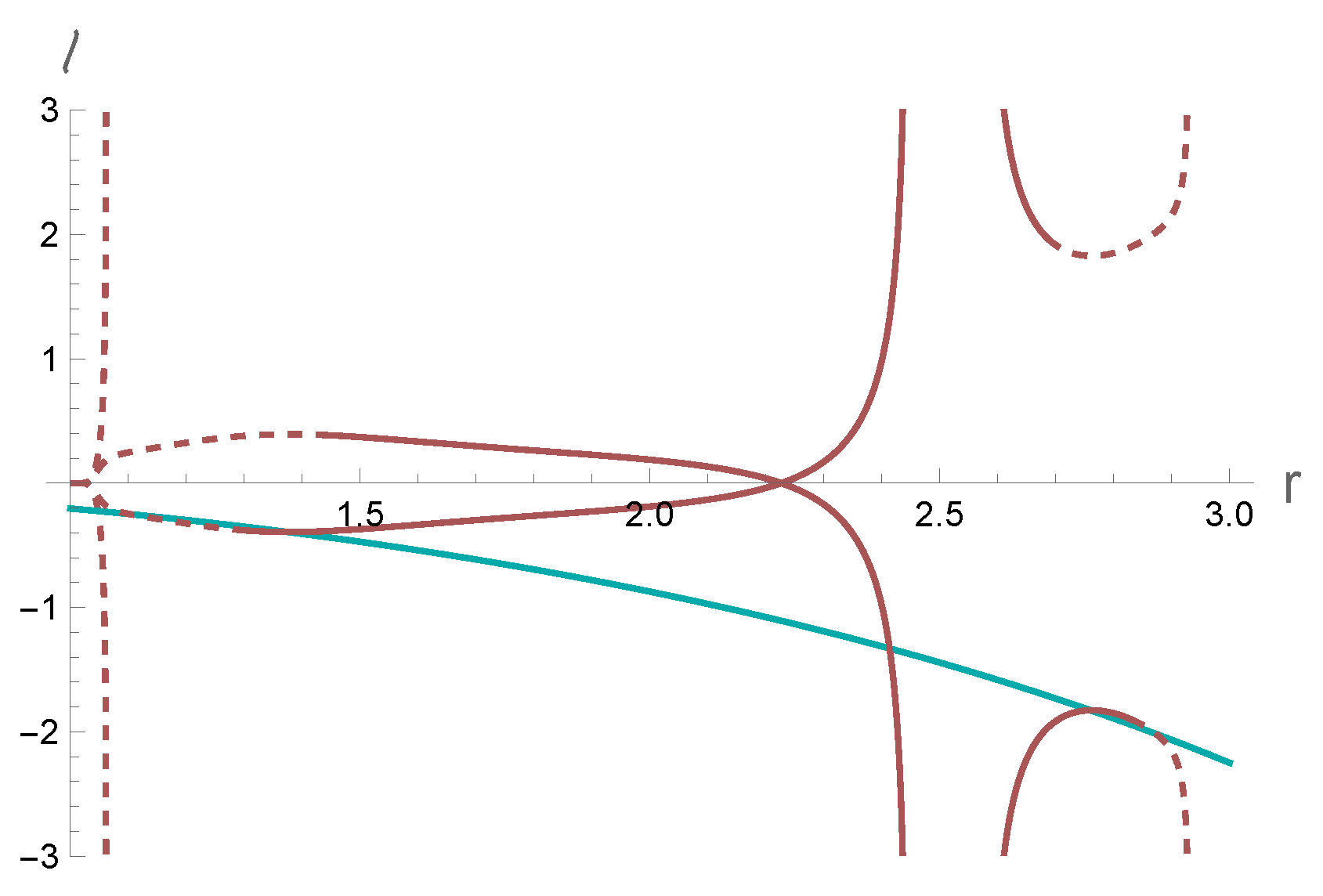
4.3. Circular Paths
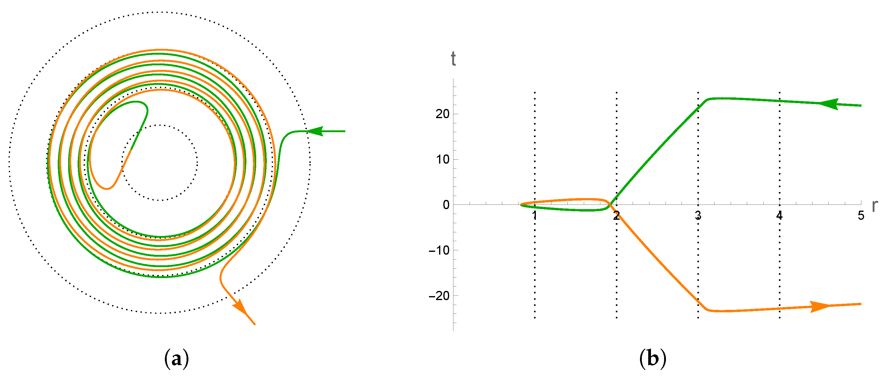
5. Free Fall to the Past
5.1. Timelike Geodesic Examples
5.2. Null Geodesic Examples
6. Discussion
Author Contributions
Funding
Data Availability Statement
Conflicts of Interest
Abbreviations
| CTCs | closed timelike curves |
Appendix A. Relative Velocity
Appendix B. 4-Acceleration Formula
Appendix C. Generalized Warp Field Construction
| 1 | Intuitively, the bubble is a topological ball, at least under the original Minkowski metric as restricted to a hypersurface . Alcubierre’s f only approaches 0 asymptotically, and hence is not compactly supported, but one might consider instead for some small constant. |
| 2 | For the special case , we have instead:
Note that for , both and must be nonzero for a nondegenerate metric, and for any nonzero vector. |
References
- Gödel, K. An Example of a New Type of Cosmological Solutions of Einstein’s Field Equations of Gravitation. Rev. Mod. Phys. 1949, 21, 447–450. [Google Scholar] [CrossRef]
- Ellis, G.F.R. Editor’s Note. Gen. Relativ. Gravit. 2000, 32, 1399–1408. [Google Scholar] [CrossRef]
- Echeverria, F.; Klinkhammer, G.; Thorne, K.S. Billiard balls in wormhole spacetimes with closed timelike curves: Classical theory. Phys. Rev. D 1991, 44, 1077–1099. [Google Scholar] [CrossRef] [PubMed]
- Friedman, J.; Morris, M.S.; Novikov, I.D.; Echeverria, F.; Klinkhammer, G.; Thorne, K.S.; Yurtsever, U. Cauchy problem in spacetimes with closed timelike curves. Phys. Rev. D 1990, 42, 1915–1930. [Google Scholar] [CrossRef] [PubMed]
- Hawking, S.W. Chronology protection conjecture. Phys. Rev. D 1992, 46, 603–611. [Google Scholar] [CrossRef] [PubMed]
- Krasnikov, S. Time machines with the compactly determined Cauchy horizon. Phys. Rev. D 2014, 90, 024067. [Google Scholar] [CrossRef]
- Deutsch, D. Quantum mechanics near closed timelike lines. Phys. Rev. D 1991, 44, 3197–3217. [Google Scholar] [CrossRef] [PubMed]
- Politzer, H.D. Path integrals, density matrices, and information flow with closed timelike curves. Phys. Rev. D 1994, 49, 3981–3989. [Google Scholar] [CrossRef] [PubMed]
- Lloyd, S.; Maccone, L.; Garcia-Patron, R.; Giovannetti, V.; Shikano, Y.; Pirandola, S.; Rozema, L.A.; Darabi, A.; Soudagar, Y.; Shalm, L.K.; et al. Closed Timelike Curves via Postselection: Theory and Experimental Test of Consistency. Phys. Rev. Lett. 2011, 106, 040403. [Google Scholar] [CrossRef] [PubMed]
- Visser, M. The Kerr spacetime: A brief introduction. arXiv 2007, arXiv:0706.0622. [Google Scholar]
- Tippett, B.K.; Tsang, D. Traversable acausal retrograde domains in spacetime. Class. Quantum Gravity 2017, 34, 095006. [Google Scholar] [CrossRef]
- Ori, A. A Class of Time-Machine Solutions with a Compact Vacuum Core. Phys. Rev. Lett. 2005, 95, 021101. [Google Scholar] [CrossRef]
- Ori, A. Formation of closed timelike curves in a composite vacuum/dust asymptotically flat spacetime. Phys. Rev. D 2007, 76, 044002. [Google Scholar] [CrossRef]
- Soen, Y.; Ori, A. Improved time-machine model. Phys. Rev. D 1996, 54, 4858–4861. [Google Scholar] [CrossRef]
- Mallary, C.; Khanna, G.; Price, R.H. Closed timelike curves and ‘effective’ superluminal travel with naked line singularities. Class. Quantum Gravity 2018, 35, 175020. [Google Scholar] [CrossRef]
- Alcubierre, M. Letter to the editor: The warp drive: Hyper-fast travel within general relativity. Class. Quantum Gravity 1994, 11, L73–L77. [Google Scholar] [CrossRef]
- Krasnikov, S.V. Hyperfast travel in general relativity. Phys. Rev. D 1998, 57, 4760–4766. [Google Scholar] [CrossRef]
- Olum, K.D. Superluminal Travel Requires Negative Energies. Phys. Rev. Lett. 1998, 81, 3567–3570. [Google Scholar] [CrossRef]
- Natário, J. Warp drive with zero expansion. Class. Quantum Gravity 2002, 19, 1157–1165. [Google Scholar] [CrossRef]
- Bobrick, A.; Martire, G. Introducing physical warp drives. Class. Quantum Gravity 2021, 38, 105009. [Google Scholar] [CrossRef]
- Everett, A.E. Warp drive and causality. Phys. Rev. D 1996, 53, 7365. [Google Scholar] [CrossRef] [PubMed]
- Ralph, T.C.; Chang, C. Spinning up a time machine. Phys. Rev. D 2020, 102, 124013. [Google Scholar] [CrossRef]
- Lobo, F.S.N.; Visser, M. Fundamental limitations on ‘warp drive’ spacetimes. Class. Quantum Gravity 2004, 21, 5871–5892. [Google Scholar] [CrossRef]
- Fermi, D.; Pizzocchero, L. A time machine for free fall into the past. Class. Quantum Gravity 2018, 35, 165003. [Google Scholar] [CrossRef]
- Misner, C.; Thorne, K.; Wheeler, J. Gravitation; W.H. Freeman and Co.: New York, NY, USA, 1973. [Google Scholar]
- Gourgoulhon, E. 3+1 Formalism in General Relativity; Springer: Berlin/Heidelberg, Germany, 2012; Volume 846. [Google Scholar] [CrossRef]
- Alcubierre, M.; Lobo, F.S.N. Warp Drive Basics. Fundam. Theor. Phys. 2017, 189, 257. [Google Scholar] [CrossRef]
- Jantzen, R.; Carini, P.; Bini, D. GEM: The User Manual: Understanding Spacetime Splittings and Their Relationships. Unpublished work. 2013. [Google Scholar]
- Hestenes, D.; Sobczyk, G. Clifford Algebra to Geometric Calculus; Springer: Berlin/Heidelberg, Germany, 1984. [Google Scholar]


Disclaimer/Publisher’s Note: The statements, opinions and data contained in all publications are solely those of the individual author(s) and contributor(s) and not of MDPI and/or the editor(s). MDPI and/or the editor(s) disclaim responsibility for any injury to people or property resulting from any ideas, methods, instructions or products referred to in the content. |
© 2024 by the authors. Licensee MDPI, Basel, Switzerland. This article is an open access article distributed under the terms and conditions of the Creative Commons Attribution (CC BY) license (https://creativecommons.org/licenses/by/4.0/).
Share and Cite
MacLaurin, C.; Costa, F.; Ralph, T.C. Falling into the Past: Geodesics in a Time Travel Metric. Universe 2024, 10, 95. https://doi.org/10.3390/universe10020095
MacLaurin C, Costa F, Ralph TC. Falling into the Past: Geodesics in a Time Travel Metric. Universe. 2024; 10(2):95. https://doi.org/10.3390/universe10020095
Chicago/Turabian StyleMacLaurin, Colin, Fabio Costa, and Timothy C. Ralph. 2024. "Falling into the Past: Geodesics in a Time Travel Metric" Universe 10, no. 2: 95. https://doi.org/10.3390/universe10020095