
Gauss’s Law and a Gravitational Wave

1
Department of Physics, University of Durham, Durham DH1 3LE, UK
2
Department of Physics and Astronomy, University of Lethbridge, Lethbridge, AB T1K 3M4, Canada
*
Author to whom correspondence should be addressed.
†
These authors contributed equally to this work.
Universe 2024, 10(2), 65; https://doi.org/10.3390/universe10020065
Submission received: 22 November 2023
/
Revised: 16 January 2024
/
Accepted: 29 January 2024
/
Published: 31 January 2024
(This article belongs to the Special Issue Quantum Gravity Phenomenology II)
Abstract
:In this paper, we discuss the semi-classical gravitational wave corrections to Gauss’s law and obtain an explicit solution for the electromagnetic potential. The gravitational wave perturbs the Coulomb potential with a function that propagates it to the asymptotics.
1. Introduction
The discovery of gravitational waves (GWs) has not only opened a window to astrophysical events, but it has also given us instruments that are sensitive enough to test very weak gravitational phenomena [1,2]. Therefore, new theoretical work acquires meaning and some of the results can be tested, thereby providing evidence for the correctness of the physical theories. In particular, quantum gravity, which has no experimental confirmation as of yet, needs to be tested. Our entire understanding of the visible matter universe is based on the standard model of particle physics, which is quantized. The quantum of the GW—the graviton—is yet to be detected, and theoretical predictions regarding it have non-renormalizable quantum interactions. What, therefore, is the story of gravity at tiny length scales? In [3], we explored a coherent state for the GW, which would help to predict semi-classical phenomena at higher length scales than the cm Planck length. Verification of the predictions from the coherent states would provide evidence for an underlying quantum world, which we hope to probe at a later time with more sophisticated instruments and understanding. On this note, we will briefly discuss a modified GW metric that was obtained in [3] and has a semi-classical correction to it. A similar computation of generalized uncertainty principle correction to a GW detector has appeared in this volume [4]. We will then solve Gauss’s law and find that there are interesting results with the GW metric when used by itself. What we will find could be interpreted as the charge density receiving a correction that is measurable. We will consider a configuration with a point charge at the origin, which thus places us in the realm of electrostatics. Coulomb’s law is valid and gives the electric field but no magnetic field. We found that if the background of this is not flat spacetime but a GW, then there is a non-zero ‘current’ generated. An interesting discussion of a similar phenomenon and its applications can be found in [5]. Note our work is also different from the example of an oscillatory electron, which is discussed in [6]. As the change in source is proportional to the GW amplitude, we studied a ‘perturbation’ of Coulomb’s law that is time-dependent and gives rise to a magnetic field. The time-dependent scalar potential does not fall off at infinity but rises with distance. The electric field’s radial component runs to zero at infinity, but the angular components rise as they have the same radial behavior as the potential; this can be measured and we will provide some numerical estimates. We also show that the magnetic potential is generated in a similar way as the electric potential. A magnetic field will be obtained from this as non-zero, though one that is very weak. In the conclusion, we will discuss the results in detail.
2. Gauss’s Law and the Gravitational Wave
We solved for Maxwell’s equation when investigating the background of a gravitational wave metric, which was corrected using semi-classical coherent states [3]. For the Maxwell field, the Lagrangian is:
where we assumed a non-trivial metric.
From the Euler–Lagrange equations, we obtained the following EoM in the presence of a four-source current :
In [3], which appeared in this volume, we found semi-classical corrections to a GW metric. We used the coherent states in a system of loop quantum gravity (LQG) [7,8], which was defined on the phase space of the LQG canonical variables, i.e., holonomies and conjugate momenta . The holonomy of the gauge connection was obtained from the exponential of a path-ordered integral of a gauge connection over a one-dimensional ‘edge’ , which formed the links of a graph; meanwhile, the momentum (built from the densitized triads ) was obtained by smearing the triads over surfaces which the edges intersected. In this calculation, we used only the momentum variables,
and the following relation:
where are the density triads; represent the space and internal SU(2) indices respectively; is the three-space metric of the background; and q is its determinant. The coherent states were also characterized using a semi-classical parameter , which is a ratio of the Planck length to the length scale of a system (here is the GW wavelength) and has a range of . For these purposes, we considered a measurable for a GW with a frequency of Hz. This, however, was too high for the observed waves (which had a frequency of 100 Hz) as their was far smaller. For the next generation of detectors which will detect higher frequency waves, see [9] for a review.
The momenta were generated by smearing the triads over the faces of a cube, which were perpendicular to the edges which were straight lines along the three axes. This type of discretization is not unique; however, with respect to the continuum limit, it serves the purpose of helping to find a semi-classical correction to the metric, as defined from the operator expectation values of the momentum (a detailed discussion on this topic can be found in [3]). The LQG-corrected metric of a gravitational wave with the polarizations of (as derived in [3]) is as follows:
The determinant of the metric was simplified to a first order in , which yielded the following:
where the semi-classical correction functions in the metric were
where refers to the straight edges along the x, y, z directions of the three spatial slices of the system [3]; represents the graph edge lengths; gives the continuum geometry; and is the dimensional gravitational constant, which is expressed in natural units as the Planck length squared. We then found the 0th component of the Maxwell’s equations in a vacuum, i.e., in the presence of no sources. In flat geometry, this gives us Gauss’s law, but in the background of the new metric, one instead obtains the following:
As the metric semi-classical corrections were proportional to the GW, these corrections were found to be functions of (which has been found as such only in [3]). However, the derivative terms were proportional to , which is a product of small quantities; therefore, we could neglect them in the first approximation. Thus, we obtained
In the approximation, we wrote the electric field as a zero-eth order field plus a small perturbation, and the RHS of the above equation could be interpreted as a source for the perturbation. The zeroeth order field was a static EM field, which was generated by a point source at the origin. Hence, we obtained
where we assumed a point source charge at the origin, or at least a charge of 1 Coulomb within a small radius (which is where our considerations were outside the radius). As the source was time-dependent, we took the perturbation to be composed of the potentials
In the Coulomb gauge , the following was yielded:
which is clearly Poisson’s equation with a time-dependent source. Seeing as the divergence of the electric field was zero and the first order in the corrections, all of the were found to be equal; as such, we can ignore the semi-classical term (=). A way through which to understand the GW-generated oscillation of the source was to observe that the charge density fluctuated with time as the volume changed.
To simplify the system, at , we solved for the equations. As such, we obtained, as the particular solution, the following:
Clearly, this potential is different in behavior to the regular spherical potential of the point-charge source at the origin. Here, the dependence makes the potential acquire different signs as it approaches the x and y axes. If we write the above equation in spherical coordinates, in which we assume a form of the potential in spherical harmonics with the same frequency as that of the GW in its time dependence, we obtain
which gives, from Gauss’s law, the following:
We then assumed that . If we keep the plane wave in the source (), then we have to use the spherical wave expansion of the function , where we obtain the following:
Using the partial wave analysis of the above RHS (with the assumption that the EM potential has the same frequency as the GW), a propagating mode was generated in the case of the oscillating sources. We also wrote the equation . We found that the ODE for was the same as the ODE for ; therefore, we dropped the second index and solved for the following equation:
The associated Legendre function is on the left and the usual Legendre function is on the right. If we take the orthonormality property of the associated Legendre functions by first multiplying with and then integrating both sides of the Equation for , we obtain
where represents the normalization constant from . Furthermore, we replaced with x for brevity. The LHS uses the orthogonality condition; but, on the RHS, the integral was difficult to compute. Given the Legendre function recursion equations [10] and integrals [11], we obtained non-zero values for and . Therefore, we found
where there were also the following constants:
There were, therefore, three independent partial waves, which gave non-zero values for the RHS of the equation and generated the ‘source’ for the EM potential of the nth angular mode. We used MAPLE to generate the solution to the above ODE, and we found a very elongated formula that contained LommelS1 and Hypergeometric functions, which, nevertheless, gave the RHS particular solution. It must be noted that, if we keep the term detailed in the above equation, the particular solution will become corrected with static functions as there are no-time dependent contributions of the first order in . As mentioned earlier, we ignored the product terms, which are equivalent to the second -order infinitesimal corrections to Gauss’s law.
The general solution is as follows:
In the above, we have as the Bessel function of the first kind, as the LommelS1 functions, and and as the Hypergeometric functions of the (2, 3) and (1, 2) type, respectively. In addition, was set to have the usual partial wave potentials of the form and , which were also the solutions of the homogeneous equation. The particular solutions represent the functions generated by the GW-induced oscillations and are propagating EM potentials. There were singularities hidden in the LommelS1 functions for the integer values of n, which we regulated. Note that we can trust only the solutions for , and this is justified as we have a semi-classical parameter and the discretization length scale, which provide a minimum length to which the geometry can be probed. The constants were
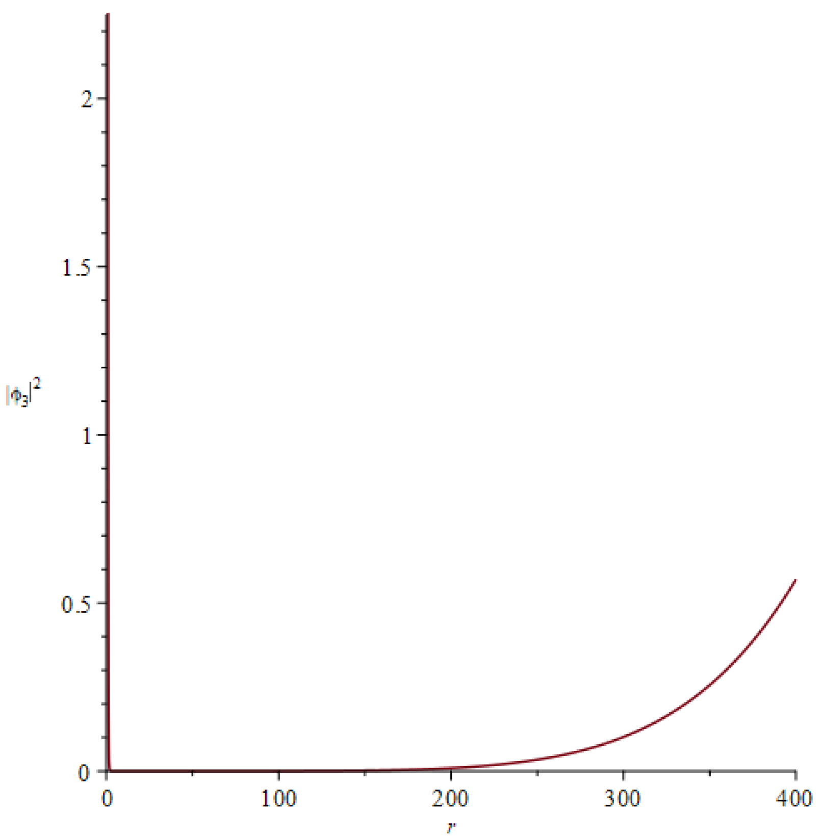
Note that the above results were true only for and higher. As the behavior of the functions for general n were difficult to plot, we simply took one representative partial wave and observed the difference from a regular solution. We took and observed the behavior of as . The function had a real component that fell of as the was obtained from the homogeneous equation solution, and an imaginary component (which was evident from the coefficients on the RHS) was the particular solution for . Additionally, as our ansatz for the potential was of the form , it was not surprising that the solution was complex. We then plotted the function to examine its asymptotic behavior. We found that, despite putting the particular solution strength as of the term, the function started increasing after a certain interval. We know that as , but the presence of GWs reverses the fall off. This behavior persists for a higher n, thus confirming our claim that the electric potential now extends to the asymptotic region.
In general, the solutions will be of the form
To obtain the observable function, one must take the real part of the summed solution. As shown above in Equation (20), is composed of solutions to the homogeneous equations of the form . In addition, for each l, there is a particular solution. It is plausible that the sum over l for the particular solution has a finite convergent answer. We tried finding a convergent answer but the summation was not simple; thus, work is still in progress. We instead used a numerical method of summing up the partial waves to some finite number. We then plotted the particular solution and summed up to , where m is some large number. This evidently represents a truncated GW wave contribution that is up to the mode in the source, but it is a good-enough approximation to what might be the real system. Therefore, we—in the following—plotted the plane wave that was summed up to , as well as showed the corresponding Coulomb potential that was generated by the system.
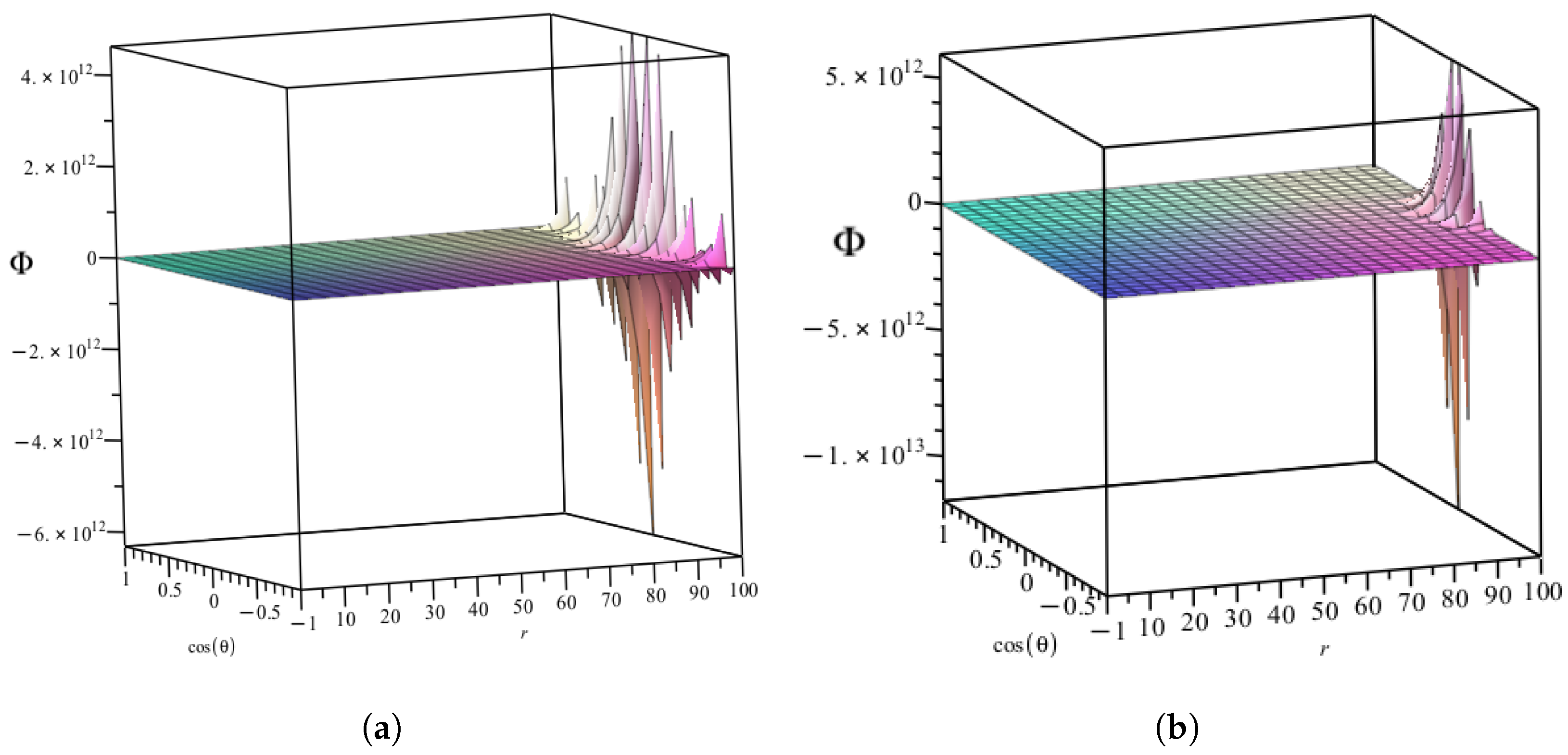
We investigated the analytic formula in Equation (20) and the partial wave summation of the spherical wave solution. We found that the potential started growing as had been observed for the solution of the potential, as shown in Figure 1. We then plotted the potential in 3d and for . This showed that the GW effect on the Coulomb potential was non-trivial and was, in principle, detectable using an electrometer, which is sensitive to the electric potential. This approach will aid in the detection of a GW in a very isolated environment.
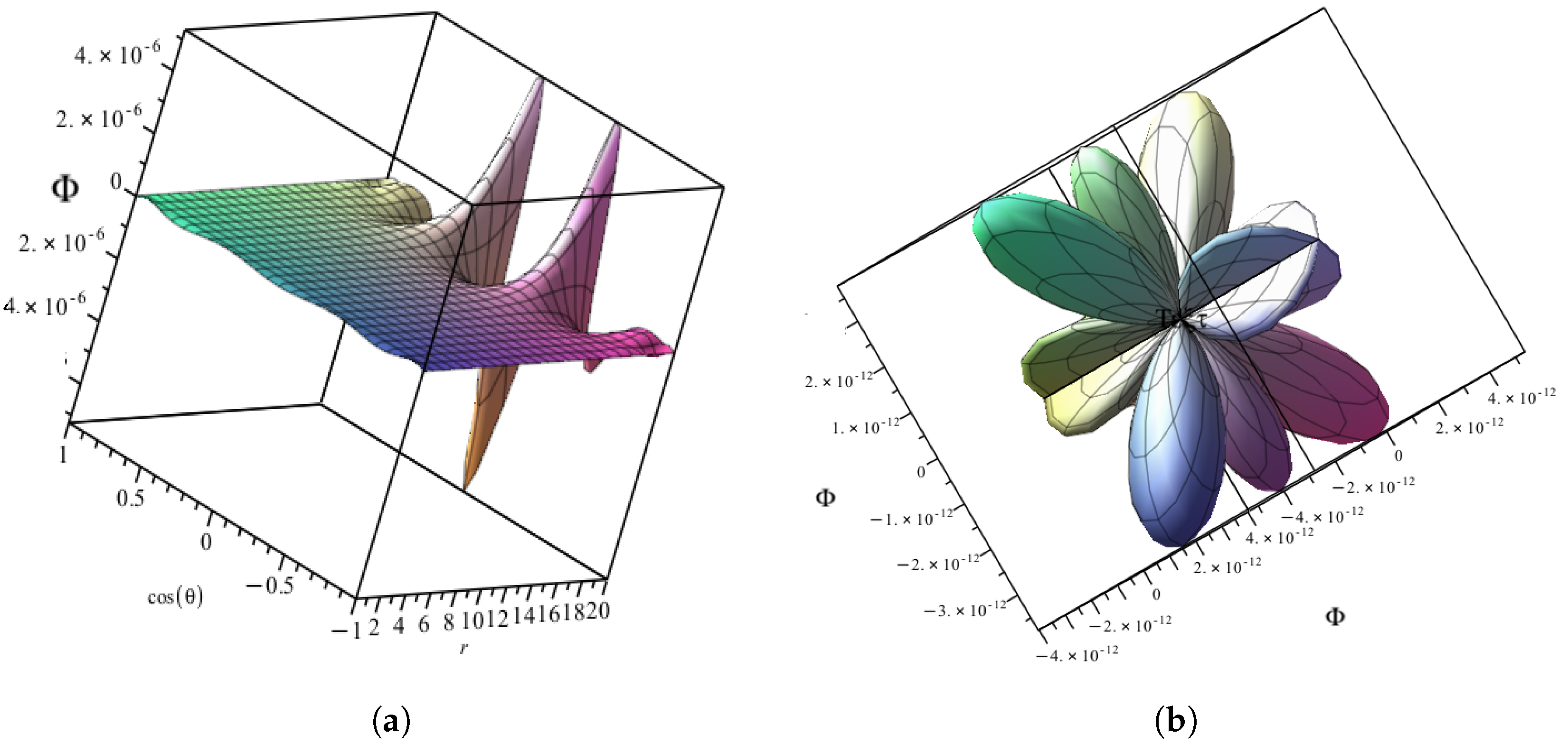
As is evident from the above plots, i.e., in Figure 2a,b (one for and another for ), the potential increased as a function of r, and the image on the axis showed oscillations due to the Legendre function. If one plots the sum over a small interval, then these features are also evident, as shown in Figure 3a. If one plots the potential on the sphere, the oscillations would of course appear as ‘petals’ in a spherical coordinates plot, as shown in Figure 3b.
The electric field defined from the above potential was expressed simply as
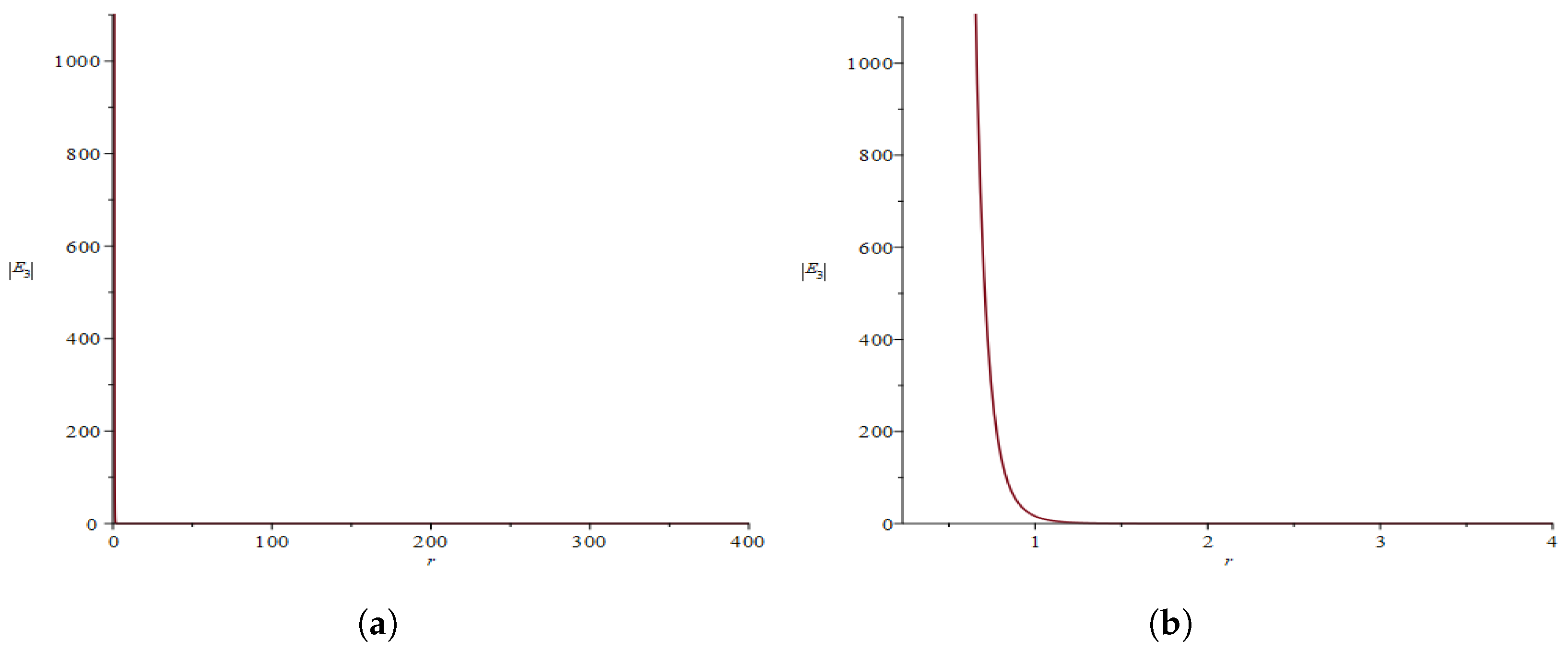
The electric field in the direction had a non-trivial derivative in the radial direction. The derivatives of and acted on the and the functions. We found that the function was the derivative of the potential function that is given in Equation (20); it was also found to be very lengthy and involved SturveH functions. Instead of quoting that, we show a graphical representation of the functions in the following Figure 4a,b for the partial wave only.
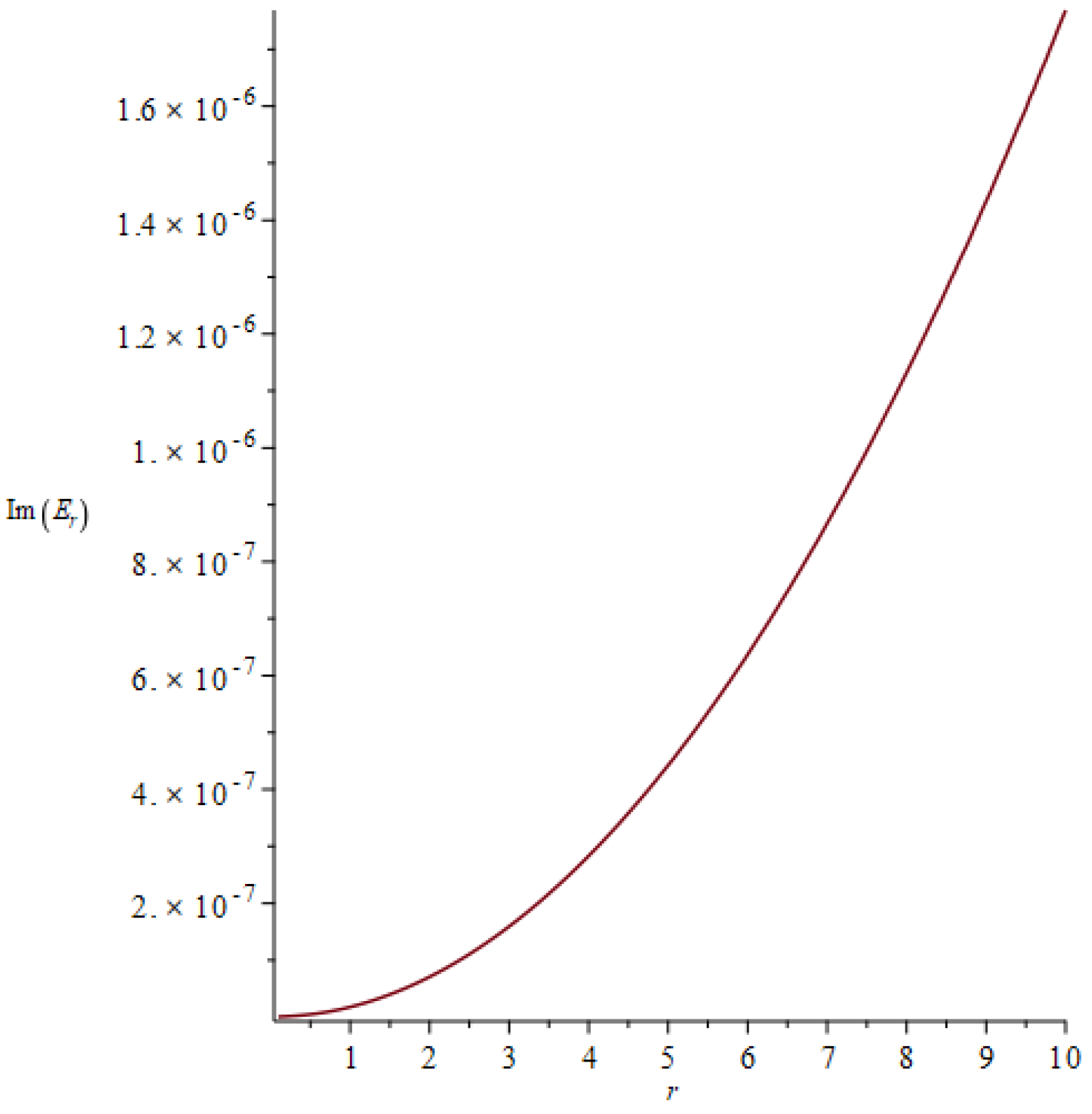
As evident from the above, the radial component decreased with distance. However, it must be mentioned that the particular part of the solution did show an increase as a function of r. As in the potential, we took the ratio of the Coulomb term and GW-induced term as . In the event that this ratio was different, the nature of the electric field’s radial component would again change. As shown in Figure 5, the contribution from the GW-induced electric field increased with r. It also remained that there were angular components of the electric field, which were generated due to the GW, and these should be detectable in an electrometer.
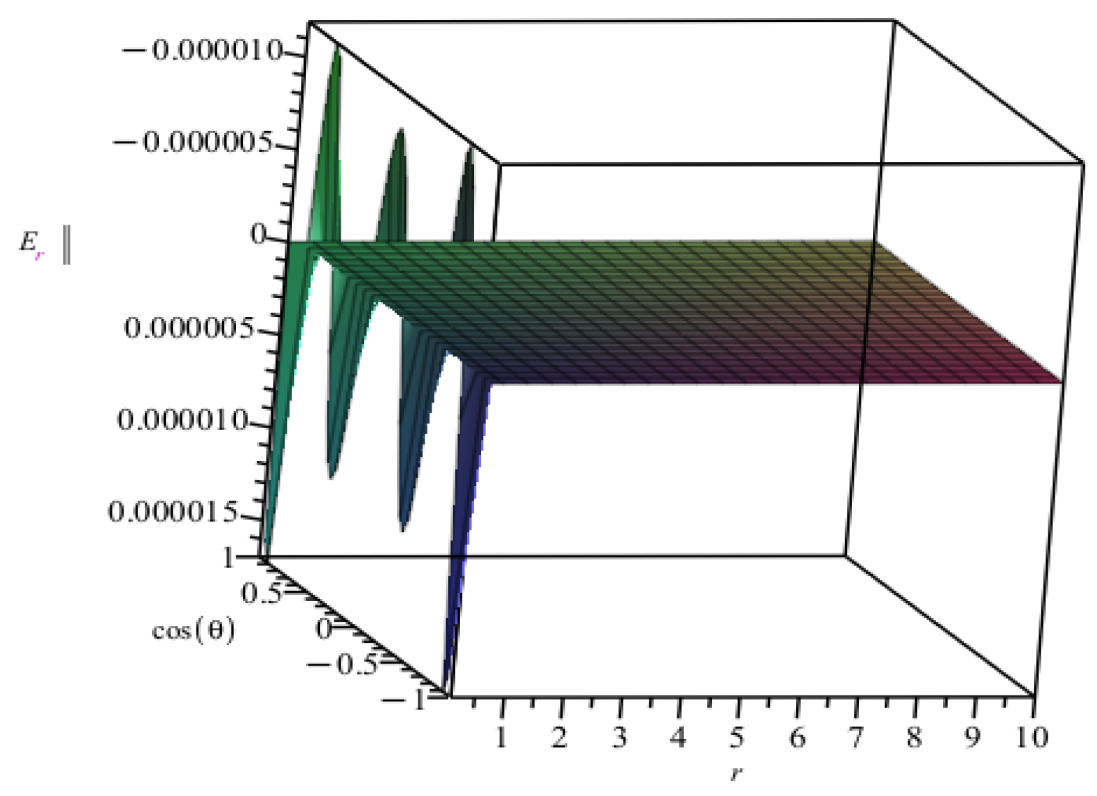
Next, we also found that the electric field’s radial component for the summed potential was . This showed behavior that was almost similar to the electric field for , where the function shows a fall off as a function of r. We plotted the particular solution of the GW-induced electric field, which is non-trivial, for k = 1, as shown in Figure 6.
Before we end this discussion, the obvious question is whether a calibrated electrometer will detect the above-generated fluctuating electric field, and the answer is yes. If we find the potential function at a distance of 10 m from the origin where a Coulomb charge has been placed (∼1) and where the GW has a frequency of 10 Hz with an amplitude of , then the component at a fixed angle being proportional to the potential is almost of a 0.1 N/C order. Small changes in the magnetic fields were detected by SQUIDS [12], we therefore needed to discuss the magnetic field generated by the GW.
In the above, we showed how a GW can modify Gauss’s law but where our electric field perturbation was time dependent. Therefore, the discussion is incomplete without discussing the magnetic field and studying the vector potential. To obtain the magnetic field, we studied Maxwell’s equations for , where i is a space component and the current density is , as we are only studying Coulomb’s law for a static source in this discussion. We found that Maxwell’s equation is as follows:
As the magnetic field was initially zero, the contribution to a non-zero magnetic field at a first order in the GW amplitude was
In the above, is the components of the Coulomb field and is the perturbations that were computed due to the GW. If we use the Lorenz gauge and write the magnetic field in terms of a Gauge potential , such that , one obtains
The above equations can be solved using the same method as the scalar potential solution for Gauss’s law. Thus, apart from modifying Gauss’s law, the GW also induces a magnetic field, and this can be calculated. We hope to discuss this in a future work. The fact that a tiny magnetic field was generated is important for detection purposes as small changes in magnetic fields can be found using SQUIDS [12].
3. Conclusions
In this short article, we have shown that the GW generates a source for a perturbation of the EM potential, which is time-dependent. The solution is complicated in form but was exactly obtained. As GWs were detected, we predicted the corrections to the Coulomb potential being of a point source charge, and we hope to find an experimental verification of our results. The semi-classical corrections to the metric described in the paper will also correct Gauss’s law in a slightly similar functional form but will also be of a next order in the perturbation. Previously, and in recent years, GW wave-induced corrections to Maxwell’s equations have been studied [12,13,14,15,16], but our results specifically discussed corrections to a static electric Coulomb potential using partial wave analysis. We also showed how a magnetic field is generated by the GW. We found that, when using numerical values, the GW-induced electric fields propagated and can be almost of an order 1. The question then is, have we already seen the GW-induced correction to Gauss’s law in some detector? To attribute the EM detection to a GW would therefore be the next task.
Funding
O.O. was funded by a MITACS summer fellowship.
Data Availability Statement
This paper did not report any experimental data.
Acknowledgments
We are grateful to Narasimha Reddy Gosala for their useful discussions.
Conflicts of Interest
The authors declare no conflict of interest.
References
- Abbott, B.P.; Abbott, R.; Abbott, T.D.; Abraham, S.; Acernese, F.; Ackley, K.; Bulik, T.; LIGO–Virgo–KAGRA Collaboration. Prospects for Observing and Localizing Gravitational-Wave Transients with Advanced LIGO, Advanced Virgo and KAGRA. Living Rev. Rel. 2020, 23, 3. [Google Scholar] [CrossRef] [PubMed]
- Saulson, P.R. Fundamentals of Interferometric Gravitational Wave Detectors; World Scientific: Singapore, 1994. [Google Scholar]
- Dasgupta, A.; Montenegro, J.L.F. Aspects of Quantum Gravity phenomenology and Astrophysics. Universe 2023, 9, 128. [Google Scholar] [CrossRef]
- Sen, S.; Bhattacharya, S.; Gangopadhay, S. Path Integral Action for a Resonant Detector of Gravitational Waves in the Generalized Uncertainty Principle Framework. Universe 2022, 8, 450. [Google Scholar] [CrossRef]
- Bruschi, D.E. Gravity-induced electric currents. arXiv 2023, arXiv:2306.03742. [Google Scholar]
- Audagnotto, G.; Keitel, C.H.; Piazza, A.D. Proportionality of gravitational and electromagnetic radiation by an electron in an intense plane wave. Phys. Rev. D 2022, 106, 076009. [Google Scholar] [CrossRef]
- Thiemann, T.; Winkler, O. Gauge field theory coherent states (GCS): II. Peakedness properties. Class. Quantum Gravity 2001, 14, 2561. [Google Scholar] [CrossRef]
- Thiemann, T. Introduction to Modern Canonical General Relativity. arXiv 2001, arXiv:0110034. [Google Scholar]
- Aggarwal, N.; Aguiar, O.D.; Bauswein, A.; Cella, G.; Clesse, S.; Cruise, A.M.; White, G. Challenges and Opportunities of Gravitational Wave Searches at MHz to GHz frequencies. Liv. Rev. Rel. 2021, 24, 4. [Google Scholar] [CrossRef]
- Gradshteyn, I.S.; Ryzhik, I.M. Tables of Integrals, Series, Products; Elsevier: Amsterdam, The Netherlands, 2007. [Google Scholar]
- Samaddar, S.N. Some Integrals Involving Associated Legendre Functions. Math. Comp. 1974, 128, 257. [Google Scholar]
- Cabral, F.; Lobo, F.S.N. Gravitational Waves and Electrodynamics: New perspectives. Eur. Phys. J. C 2017, 77, 237. [Google Scholar] [CrossRef] [PubMed]
- Patel, A.; Dasgupta, A. Interaction of Electromagnetic field with a Gravitational wave in Minkowski and de-Sitter space-time. In General Relativity and Quantum Cosmology; Cornell University: Ithaca, NY, USA, 2021. [Google Scholar]
- Kim, D.; Park, C. Detection of gravitational waves by light perturbation. Eur. Phys. J. C 2021, 81, 563. [Google Scholar] [CrossRef]
- Ganjali, M.A.; Sedaghatmanesh, Z. Laser interferometer in presence of scalar field on gravitational wave background. Class. Quant.Grav. 2021, 38, 105010. [Google Scholar] [CrossRef]
- Calura, M.; Montinari, E. Exact Solution to the homogeneous Maxwell Equations in the Field of a Gravitational Wave in Linearized Theory. Class. Quant. Grav. 1999, 16, 643–652. [Google Scholar] [CrossRef]
Figure 1.
The modulus square of the potential for .

Figure 2.
Real parts of . (a) Potential with partial modes summed from , . (b) Potential with the partial modes summed for , .
Figure 2.
Real parts of . (a) Potential with partial modes summed from , . (b) Potential with the partial modes summed for , .

Figure 3.
Real parts of . (a) Potential with partial modes summed from and plotted for k = 1, r = [0, 20], . (b) Potential with partial modes summed for and plotted in , k = 1, r = 1.
Figure 3.
Real parts of . (a) Potential with partial modes summed from and plotted for k = 1, r = [0, 20], . (b) Potential with partial modes summed for and plotted in , k = 1, r = 1.

Figure 4.
Magnitude of the radial electric field solution for . (a) Magnitude of for ; r = [0, 400]. (b) The field for .
Figure 4.
Magnitude of the radial electric field solution for . (a) Magnitude of for ; r = [0, 400]. (b) The field for .

Figure 5.
The GW-induced electric field radial component for , k = 1.

Figure 6.
The GW-induced electric field radial component for the partial wave summed as , k = 1.

Disclaimer/Publisher’s Note: The statements, opinions and data contained in all publications are solely those of the individual author(s) and contributor(s) and not of MDPI and/or the editor(s). MDPI and/or the editor(s) disclaim responsibility for any injury to people or property resulting from any ideas, methods, instructions or products referred to in the content. |
© 2024 by the authors. Licensee MDPI, Basel, Switzerland. This article is an open access article distributed under the terms and conditions of the Creative Commons Attribution (CC BY) license (https://creativecommons.org/licenses/by/4.0/).
Share and Cite
MDPI and ACS Style
Odutola, O.; Dasgupta, A. Gauss’s Law and a Gravitational Wave. Universe 2024, 10, 65. https://doi.org/10.3390/universe10020065
AMA Style
Odutola O, Dasgupta A. Gauss’s Law and a Gravitational Wave. Universe. 2024; 10(2):65. https://doi.org/10.3390/universe10020065
Chicago/Turabian StyleOdutola, Olamide, and Arundhati Dasgupta. 2024. "Gauss’s Law and a Gravitational Wave" Universe 10, no. 2: 65. https://doi.org/10.3390/universe10020065
Note that from the first issue of 2016, this journal uses article numbers instead of page numbers. See further details here.