
Predicting the Spread of SARS-CoV-2 in Italian Regions: The Calabria Case Study, February 2020–March 2022


Abstract
:1. Introduction
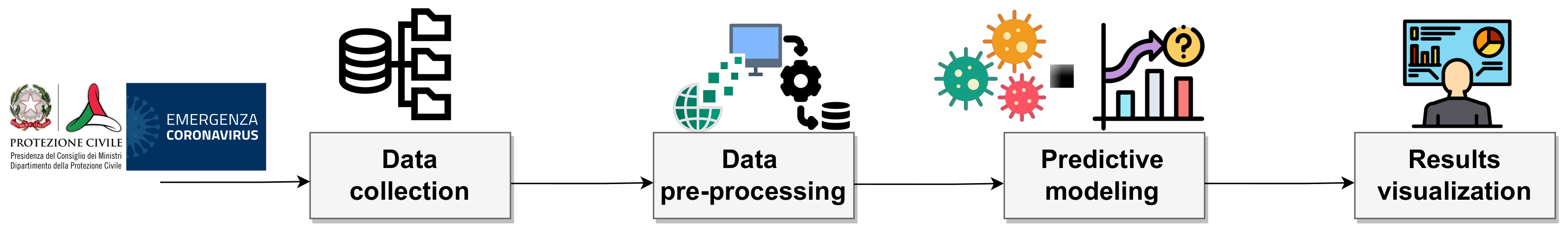
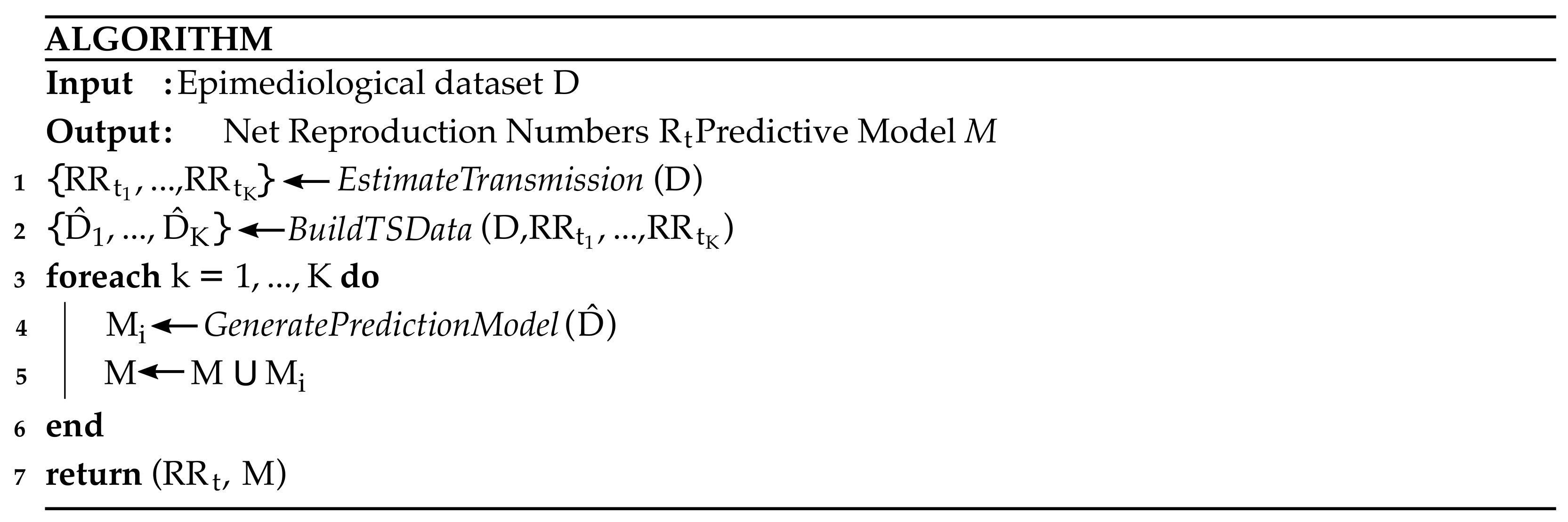
2. Materials and Methods
Software
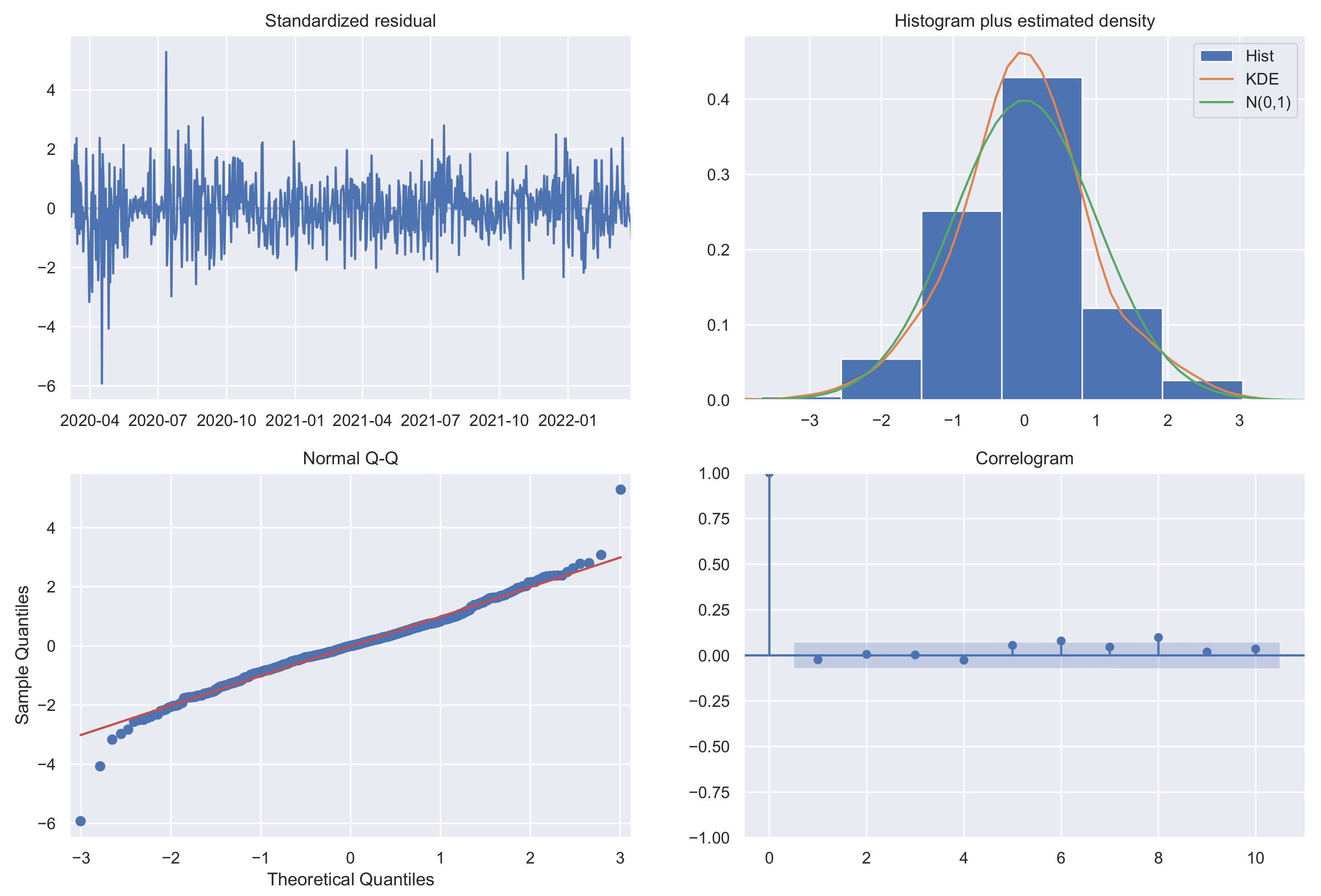
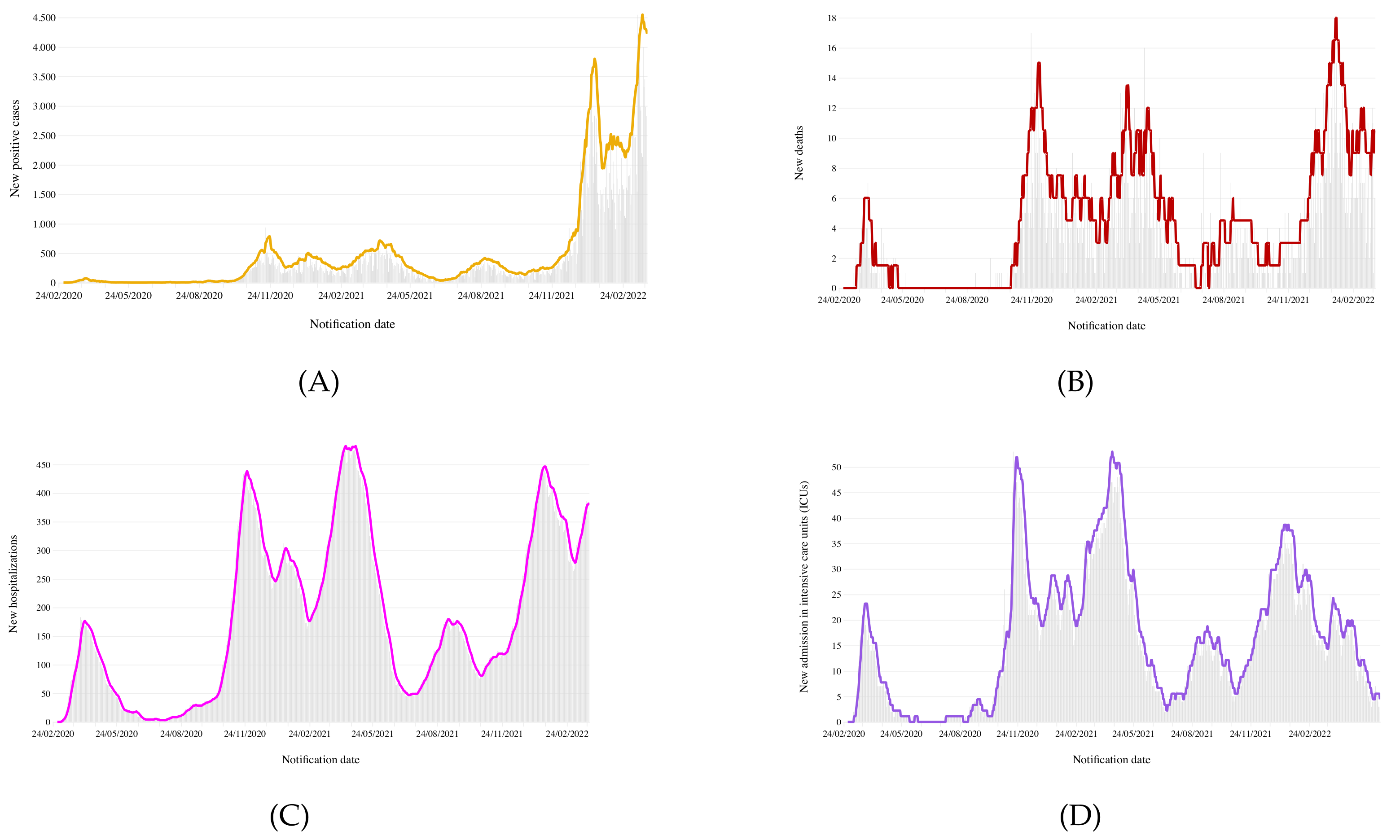
3. Results
4. Discussion
5. Conclusions
Author Contributions
Funding
Institutional Review Board Statement
Informed Consent Statement
Data Availability Statement
Conflicts of Interest
References
- Pneumonia of Unknown Cause—China. Available online: https://www.who.int/csr/don/05-january-2020-pneumonia-of-unkown-cause-china/en/ (accessed on 22 March 2022).
- Listings of WHO’s Response to COVID-19. Available online: https://www.who.int/news-room/detail/29-06-2020-covidtimeline (accessed on 20 March 2022).
- Tracking SARS-CoV-2 Variants. Available online: https://www.who.int/en/activities/tracking-SARS-CoV-2-variants/ (accessed on 20 March 2022).
- Update on Omicron. Available online: https://www.who.int/news/item/28-11-2021-update-on-omicron (accessed on 20 March 2022).
- Statement on Omicron Sublineage, BA.2. Available online: https://www.who.int/news/item/22-02-2022-statement-on-omicron-sublineage-ba.2 (accessed on 20 March 2022).
- Four Possible Cases of BA.2.2 Omicron Sub-Variant Detected in Thailand no Cause for Alarm. Available online: https://www.thaipbsworld.com/four-possible-cases-of-ba-2-2-sub-variant-detected-in-thailand-no-cause-for-alarm/ (accessed on 20 March 2022).
- Adeola, A.M.; Botai, J.O.; Rautenbach, H.; Adisa, O.M.; Ncongwane, K.P.; Botai, C.M.; Adebayo-Ojo, T.C. Climatic variables and malaria morbidity in mutale local municipality, South Africa: A 19-year data analysis. Int. J. Environ. Res. Public Health 2017, 14, 1360. [Google Scholar] [CrossRef] [PubMed] [Green Version]
- Choi, S.B.; Ahn, I. Forecasting seasonal influenza-like illness in South Korea after 2 and 30 weeks using Google Trends and influenza data from Argentina. PLoS ONE 2020, 15, e0233855. [Google Scholar] [CrossRef] [PubMed]
- He, J.; He, J.; Han, Z.; Teng, Y.; Zhang, W.; Yin, W. Environmental Determinants of Hemorrhagic Fever with Renal Syndrome in High-Risk Counties in China: A Time Series Analysis (2002–2012). Am. J. Trop. Med. Hyg. 2018, 99, 1262. [Google Scholar] [CrossRef] [PubMed] [Green Version]
- Watad, A.; Watad, S.; Mahroum, N.; Sharif, K.; Amital, H.; Bragazzi, N.L.; Adawi, M. Forecasting the West Nile virus in the United States: An extensive novel data streams–based time series analysis and structural equation modeling of related digital searching behavior. JMIR Public Health Surveill. 2019, 5, e9176. [Google Scholar] [CrossRef] [Green Version]
- Duan, Y.; Huang, X.L.; Wang, Y.J.; Zhang, J.Q.; Zhang, Q.; Dang, Y.W.; Wang, J. Impact of meteorological changes on the incidence of scarlet fever in Hefei City, China. Int. J. Biometeorol. 2016, 60, 1543–1550. [Google Scholar] [CrossRef]
- Zhao, Y.; Li, R.; Qiu, J.; Sun, X.; Gao, L.; Wu, M. Prediction of human brucellosis in China Based on temperature and NDVI. Int. J. Environ. Res. Public Health 2019, 16, 4289. [Google Scholar] [CrossRef] [Green Version]
- Chaurasia, V.; Pal, S. COVID-19 pandemic: ARIMA and regression model-based worldwide death cases predictions. SN Comput. Sci. 2020, 1, 1–12. [Google Scholar]
- Tan, C.V.; Singh, S.; Lai, C.H.; Zamri, A.S.S.M.; Dass, S.C.; Aris, T.B.; Ibrahim, H.M.; Gill, B.S. Forecasting COVID-19 Case Trends Using SARIMA Models during the Third Wave of COVID-19 in Malaysia. Int. J. Environ. Res. Public Health 2022, 19, 1504. [Google Scholar] [CrossRef]
- Cori, A.; Ferguson, N.M.; Fraser, C.; Cauchemez, S. A new framework and software to estimate time-varying reproduction numbers during epidemics. Am. J. Epidemiol. 2013, 178, 1505–1512. [Google Scholar]
- Durbin, J.; Koopman, S.J. Time Series Analysis by State Space Methods; OUP Oxford: Oxford, UK, 2012; Volume 38. [Google Scholar]
- De Gooijer, J.G.; Abraham, B.; Gould, A.; Robinson, L. Methods for determining the order of an autoregressive-moving average process: A survey. Int. Stat. Rev. Int. Stat. 1985, 53, 301–329. [Google Scholar] [CrossRef]
- Elliott, G.; Rothenberg, T.J.; Stock, J.H. Efficient Tests for an Autoregressive Unit Root; NBER: Cambridge, MA, USA, 1992. [Google Scholar]
- Italian COVID-19 Data Repository. Available online: https://github.com/pcm-dpc/COVID-19 (accessed on 25 March 2022).
- From Infection Report to Vaccines: All DATA on the Covid Emergency in Calabria on a Single Platform. Available online: https://www2.unical.it/portale/portaltemplates/view/view.cfm?109945 (accessed on 25 March 2022).
- Bonifazi, G.; Lista, L.; Menasce, D.; Mezzetto, M.; Pedrini, D.; Spighi, R.; Zoccoli, A. A simplified estimate of the effective reproduction number Rt using its relation with the doubling time and application to Italian COVID-19 data. Eur. Phys. J. Plus 2021, 136, 1–14. [Google Scholar] [CrossRef] [PubMed]
- Cereda, D.; Tirani, M.; Rovida, F.; Demicheli, V.; Ajelli, M.; Poletti, P.; Trentini, F.; Guzzetta, G.; Marziano, V.; Barone, A.; et al. The early phase of the COVID-19 outbreak in Lombardy, Italy. arXiv 2020, arXiv:2003.09320. [Google Scholar]
- Pavlícek, T.; Rehak, P.; Král, P. Oscillatory dynamics in infectivity and death rates of COVID-19. Msystems 2020, 5, e00700-20. [Google Scholar] [CrossRef] [PubMed]
- Huang, J.; Liu, X.; Zhang, L.; Zhao, Y.; Wang, D.; Gao, J.; Lian, X.; Liu, C. The oscillation-outbreaks characteristic of the COVID-19 pandemic. Natl. Sci. Rev. 2021, 8, nwab100. [Google Scholar] [CrossRef]
- Bukhari, Q.; Jameel, Y.; Massaro, J.M.; D’Agostino, R.B.; Khan, S. Periodic oscillations in daily reported infections and deaths for coronavirus disease 2019. JAMA Netw. Open 2020, 3, e2017521. [Google Scholar] [CrossRef]
- ArunKumar, K.; Kalaga, D.V.; Kumar, C.M.S.; Chilkoor, G.; Kawaji, M.; Brenza, T.M. Forecasting the dynamics of cumulative COVID-19 cases (confirmed, recovered and deaths) for top-16 countries using statistical machine learning models: Auto-Regressive Integrated Moving Average (ARIMA) and Seasonal Auto-Regressive Integrated Moving Average (SARIMA). Appl. Soft Comput. 2021, 103, 107161. [Google Scholar]
- Knaub, J.R., Jr. Essential Heteroscedasticity. 2017. Available online: https://www.researchgate.net/publication/32853387_Essential_Heteroscedasticity (accessed on 28 May 2022).
- Box, G.E.; Cox, D.R. An analysis of transformations. J. R. Stat. Soc. Ser. B (Methodol.) 1964, 26, 211–243. [Google Scholar] [CrossRef]
- Nontapa, C.; Kesamoon, C.; Kaewhawong, N.; Intrapaiboon, P. A New Time Series Forecasting Using Decomposition Method with SARIMAX Model. In Proceedings of the International Conference on Neural Information Processing, Bangkok, Thailand, 18–22 November 2020; Springer: Berlin/Heidelberg, Germany, 2020; pp. 743–751. [Google Scholar]
- Abenavoli, L.; Cinaglia, P.; Luzza, F.; Gentile, I.; Boccuto, L. Epidemiology of coronavirus disease outbreak: The Italian trends. Rev. Recent Clin. Trials 2020, 15, 87–92. [Google Scholar] [CrossRef]
- Abenavoli, L.; Cinaglia, P.; Procopio, A.C.; Serra, R.; Aquila, I.; Zanza, C.; Longhitano, Y.; Artico, M.; Larussa, T.; Boccuto, L.; et al. SARS-CoV-2 Spread Dynamics in Italy: The Calabria Experience. Rev. Recent Clin. Trials 2021, 16, 309–315. [Google Scholar] [CrossRef]
- Guzzetta, G.; Riccardo, F.; Marziano, V.; Poletti, P.; Trentini, F.; Bella, A.; Andrianou, X.; Del Manso, M.; Fabiani, M.; Bellino, S.; et al. Impact of a nationwide lockdown on SARS-CoV-2 transmissibility, Italy. Emerg. Infect. Dis. 2021, 27, 267. [Google Scholar] [CrossRef]
- Branda, F. Impact of the additional/booster dose of COVID-19 vaccine against severe disease during the epidemic phase characterized by the predominance of the Omicron variant in Italy, December 2021—May 2022. medRxiv 2022. [Google Scholar] [CrossRef]
- Yadav, S.K.; Akhter, Y. Statistical Modeling for the Prediction of Infectious Disease Dissemination With Special Reference to COVID-19 Spread. Front. Public Health 2021, 680. [Google Scholar] [CrossRef] [PubMed]
- Hamzah, F.B.; Lau, C.; Nazri, H.; Ligot, D.V.; Lee, G.; Tan, C.L.; Shaib, M.; Zaidon, U.H.B.; Abdullah, A.B.; Chung, M.H.; et al. CoronaTracker: Worldwide COVID-19 outbreak data analysis and prediction. Bull. World Health Organ. 2020, 1, 1–32. [Google Scholar]
- Flaxman, S.; Mishra, S.; Gandy, A.; Unwin, H.J.T.; Mellan, T.A.; Coupland, H.; Whittaker, C.; Zhu, H.; Berah, T.; Eaton, J.W.; et al. Estimating the effects of non-pharmaceutical interventions on COVID-19 in Europe. Nature 2020, 584, 257–261. [Google Scholar] [CrossRef] [PubMed]
- Giordano, G.; Blanchini, F.; Bruno, R.; Colaneri, P.; Di Filippo, A.; Di Matteo, A.; Colaneri, M. Modelling the COVID-19 epidemic and implementation of population-wide interventions in Italy. Nat. Med. 2020, 26, 855–860. [Google Scholar] [CrossRef]
- Lin, Q.; Zhao, S.; Gao, D.; Lou, Y.; Yang, S.; Musa, S.S.; Wang, M.H.; Cai, Y.; Wang, W.; Yang, L.; et al. A conceptual model for the coronavirus disease 2019 (COVID-19) outbreak in Wuhan, China with individual reaction and governmental action. Int. J. Infect. Dis. 2020, 93, 211–216. [Google Scholar] [CrossRef]


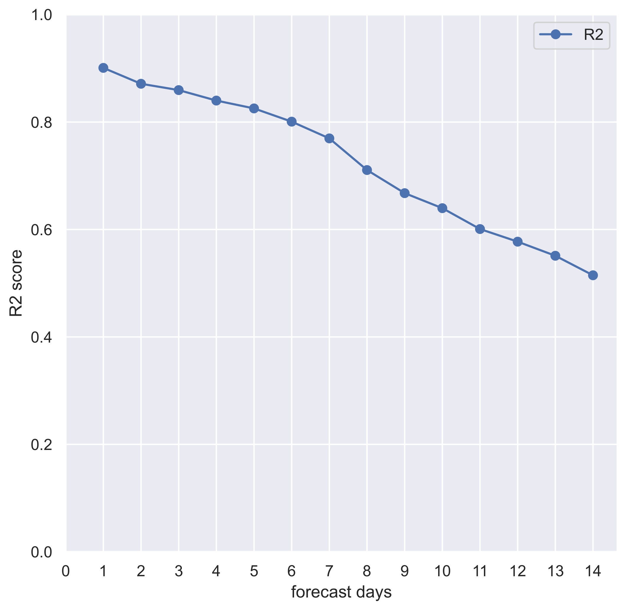
| Forecasted Days | |
|---|---|
| 1 | 0.90 |
| 2 | 0.87 |
| 3 | 0.86 |
| 4 | 0.84 |
| 5 | 0.82 |
| 6 | 0.80 |
| 7 | 0.77 |
| 8 | 0.71 |
| 9 | 0.67 |
| 10 | 0.64 |
| 11 | 0.60 |
| 12 | 0.58 |
| 13 | 0.55 |
| 14 | 0.51 |
Publisher’s Note: MDPI stays neutral with regard to jurisdictional claims in published maps and institutional affiliations. |
© 2022 by the authors. Licensee MDPI, Basel, Switzerland. This article is an open access article distributed under the terms and conditions of the Creative Commons Attribution (CC BY) license (https://creativecommons.org/licenses/by/4.0/).
Share and Cite
Branda, F.; Abenavoli, L.; Pierini, M.; Mazzoli, S. Predicting the Spread of SARS-CoV-2 in Italian Regions: The Calabria Case Study, February 2020–March 2022. Diseases 2022, 10, 38. https://doi.org/10.3390/diseases10030038
Branda F, Abenavoli L, Pierini M, Mazzoli S. Predicting the Spread of SARS-CoV-2 in Italian Regions: The Calabria Case Study, February 2020–March 2022. Diseases. 2022; 10(3):38. https://doi.org/10.3390/diseases10030038
Chicago/Turabian StyleBranda, Francesco, Ludovico Abenavoli, Massimo Pierini, and Sandra Mazzoli. 2022. "Predicting the Spread of SARS-CoV-2 in Italian Regions: The Calabria Case Study, February 2020–March 2022" Diseases 10, no. 3: 38. https://doi.org/10.3390/diseases10030038