An Embedded Platform for Positioning and Obstacle Detection for Small Unmanned Aerial Vehicles

Abstract

Unmanned Aerial Vehicles (UAV) with on-board augmentation systems (UAS, Unmanned Aircraft System) have penetrated into civil and general-purpose applications, due to advances in battery technology, control components, avionics and rapidly falling prices. This paper describes the conceptual design and the validation campaigns performed for an embedded precision Positioning, field mapping, Obstacle Detection and Avoiding (PODA) platform, which uses commercial-off-the-shelf sensors, i.e., a 10-Degrees-of-Freedom Inertial Measurement Unit (10-DoF IMU) and a Light Detection and Ranging (LiDAR), managed by an Arduino Mega 2560 microcontroller with Wi-Fi capabilities. The PODA system, designed and tested for a commercial small quadcopter (Parrot Drones SAS Ar.Drone 2.0, Paris, France), estimates position, attitude and distance of the rotorcraft from an obstacle or a landing area, sending data to a PC-based ground station. The main design issues are presented, such as the necessary corrections of the IMU data (i.e., biases and measurement noise), and Kalman filtering techniques for attitude estimation, data fusion and position estimation from accelerometer data. The real-time multiple-sensor optimal state estimation algorithm, developed for the PODA platform and implemented on the Arduino, has been tested in typical aerospace application scenarios, such as General Visual Inspection (GVI), automatic landing and obstacle detection. Experimental results and simulations of various missions show the effectiveness of the approach.

1. Introduction

Flexibility, safety, customizability, high mobility and increasingly low costs, together with efforts in the fields of innovative materials, energy storage, sensors, imaging devices, electronics and computer science, have resulted in the last decade in a phenomenal development of consumer-grade and professional-grade semi-autonomous (Remotely Piloted Aircraft Systems, RPAS) or autonomous aerial vehicles (Unmanned Aircraft Systems, UAS), as well as remotely operated vehicles for ground and sea applications (terrestrial rovers, unmanned ships, underwater drones) [1,2,3]. Research on UASs has developed very rapidly due to the wide number of military and civilian applications [4,5,6,7], and to the new challenges presented by different mission scenarios and flight profiles, such as low-elevation flights, hovering, high-dynamic maneuvers, site revisiting, etc. In particular, rotary-wing UASs have been shown to benefit with regards to easier landing and takeoff, improved maneuverability, and capabilities of infrastructure inspection or the monitoring of small areas. Therefore, much effort is being put into raising the level of autonomy of unmanned vehicles, devising strategies for low-level autonomous flight control, positioning and environment perception, as well as high-level path planning, navigation and obstacle detection, with vision-based techniques or low-cost sensor arrangements (inertial, sonic, imaging, active radars, etc.) [8,9,10,11,12], all of which has motivated the development of specialized control architectures and solutions [13,14]. The implementation of a UAV intelligent system requires autonomous navigation, control and manoeuvring algorithms in dynamic environments (for autonomous or remotely piloted modes), in order to achieve satisfactory performances in the framework of the selected mission [15,16,17,18].

This work, extending the preliminary conceptual design recently presented in a congress paper [19], deals with the development of a UAS with a Positioning, field mapping, Obstacle Detection and Avoiding (PODA) embedded system [20], exploiting lightweight, low-cost and fast-response sensors. The chosen sensors are a 10-Degrees-of-Freedom (DoF) Inertial Measurement Unit (IMU) and a Light Detection and Ranging (LiDAR) sensor. LiDAR sensors, first used in remote sensing applications, have been proposed for the effective assessment of landing zones for small helicopters [21], but recent advances in LiDAR technology have allowed UAV users to load reliable, small, low-price sensors [22].

In this investigation, the LiDAR is used for measuring the distance from the ground, whereas the IMU, using a combination of accelerometers, gyroscopes and magnetometers, allows us to estimate the platform velocity, attitude and gravitational forces [23,24,25]. The platform is modeled as a linear dynamic system perturbed by white Gaussian noise, with measurements linearly related to the state but corrupted by additive white Gaussian noise. With these assumptions, an optimal estimation (in the sense of minimum mean squared estimation error) of the system state variables from corrupted sensor readings (acceleration measurements) is achieved by real-time Kalman filtering, implemented on a microcontroller (Arduino Mega 2560, Arduino Srl, Monza, Italy). With respect to the other experimental configurations previously developed by the authors [26,27], additional information provided by the LiDAR and IMU gives more accurate attitude estimations and position evolution.

A block diagram of the PODA system is depicted in Figure 1, in which data acquired from the sensors are managed by the Arduino board, which in turn hosts the algorithms and the functions shown in the blocks. The estimates of position, $\widehat{\mathit{x}}={\left(x,y,z\right)}^T$, attitude, $\widehat{\mathit{\psi }}={\left(\eta ,\vartheta ,\phi \right)}^T$ (roll, pitch and yaw angles) and distance, $\widehat{d}$, are used for obstacle detection and flight planning. These capabilities are needed for typical UAS applications, such as general visual inspection (GVI) [28], Detect-and-Avoid (DAA) [29] and autonomous landing [30].

The content of the paper is as follows. After this Introduction, Section 2 describes the commercial quadcopter (Parrot AR.Drone 2.0) used in this study, together with the PODA setup (sensors, microcontroller, and mathematical models for accelerometer calibration and system state estimation). Section 3 is devoted to experimental results and system validation, while conclusions and ideas for further work are outlined in Section 4.

2. Materials and Methods

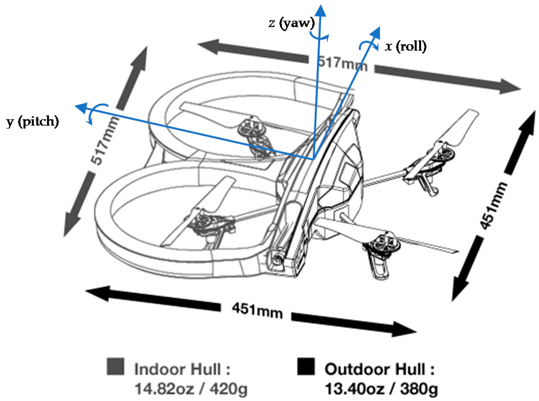
2.1. Unmanned Aerial Vehicle

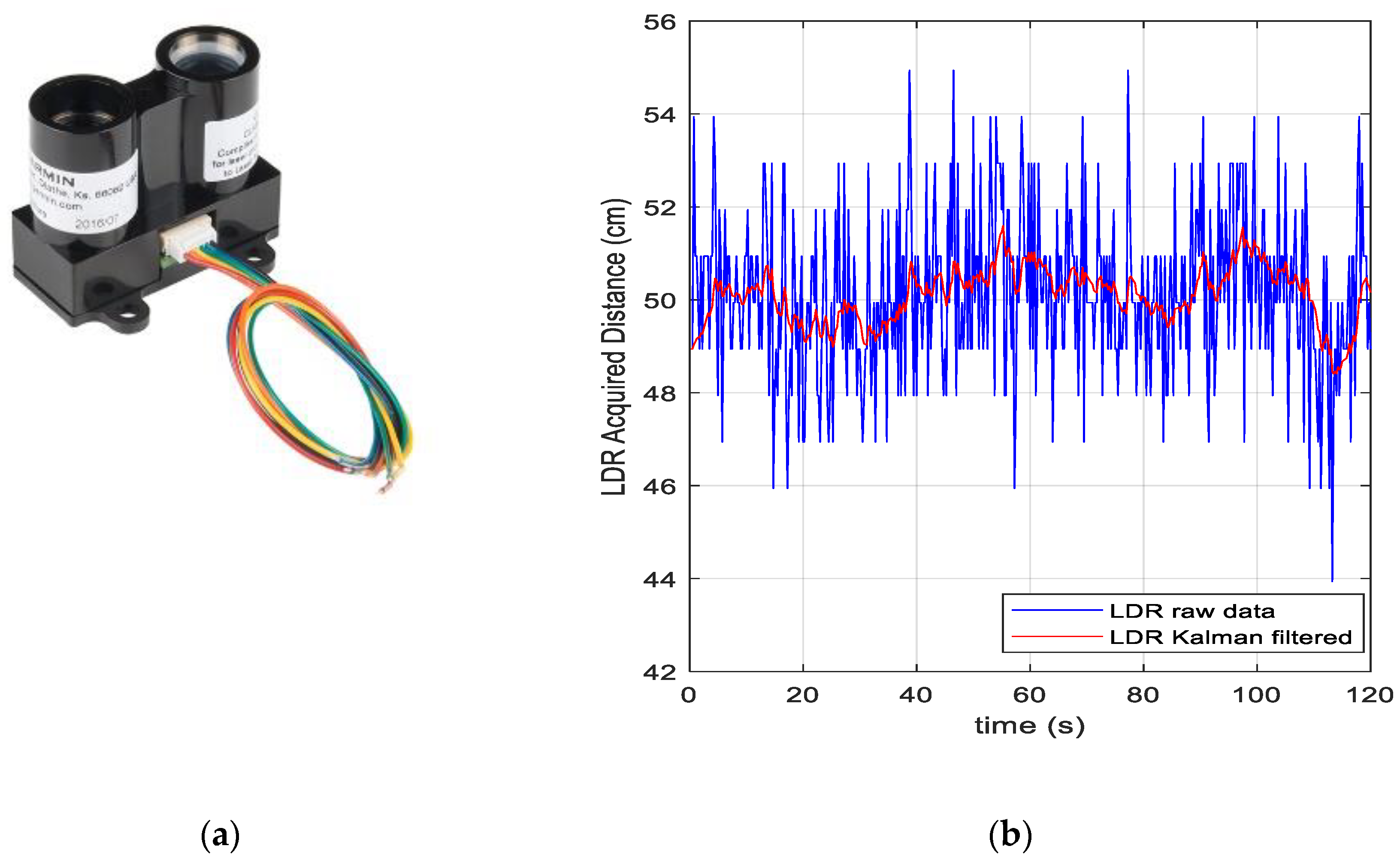
The commercial UAV selected for this research is the Parrot AR.Drone 2.0, shown in Figure 2, a small quad-rotor of the Micro UAV (MUAV, weight 0.1–1 kg, length 0.1–1 m) class. Since its inception, this fully electric quadcopter, originally designed for augmented reality games, caught the attention of several universities and research groups as a platform for educational and robotic research [30,31,32], due to its carbon-fiber support structure which consolidates modern aeronautic technology, a rigid design and easy maintainability into a very versatile vehicle. The AR.Drone 2.0 has four high-efficiency propellers installed on direct-current brushless motors (14.5-W power absorption, 28,500 rev/min) which allow the drone to attain speeds of over 5 m/s. The vehicle is equipped with a control computer based on the 1-GHz ARM Cortex A8 processor, with up to 1 GB of RAM and a software interface provided by the manufacturer, which allows communication with the drone via standard Wi-Fi networks (b, g or n). The aircraft is controllable using a PC, a tablet or a smartphone, and can also be operated outdoors during calm weather conditions (little or no wind). Two 1500-mAh high-density lythium polymer batteries can provide up to 36 min of flight [33]. Both the control computer and the sensor suite of the drone (a 10-DoF IMU, an altitude ultrasound sensor, a bottom camera for measuring the ground speed) can be bypassed, allowing the user to build a customized programmable control board. The total mass without payload is 420 g with external frame (indoor hull), 380 g with internal frame (outdoor hull). The outdoor hull configuration was used during the experimental activities, gaining about 40 g (the cover weight) for the PODA system.

2.2. LiDAR Sensor

The small, low-power, low-cost Garmin LiDAR-Lite v3 uses pulse trains of near-infrared laser signals (with a 905-nm nominal wavelength and a 10-kHz to 20-kHz pulse train repetition frequency) to measure distances by calculating the round-trip time delay of the light pulses reflected by a target. Exclusive signal processing algorithms are used to achieve high sensitivity, speed and accuracy [34]; among them, the sensor implements a receiver bias correction procedure which takes into account changing ambient light levels and optimizes sensitivity. The device runs at 5 Vdc, with typical current absorption of 135 mA in continuous operation and a total laser peak power of 1.3 W, and it has a two-wire I²C-compatible serial interface [35]. It acquires data with up to a 400-kHz update rate (Fast Mode data transfer) and can be connected to an I²C bus as a slave device, under the control of an I²C master device. The sensor range is 0–40 m with a target reflecting 70% of the incident laser light, and the beam diameter at the laser aperture is 12 mm × 2 mm.

Figure 3 shows typical LiDAR-derived measurements, from an obstacle at a nominal distance of 50 cm. Data were collected in static conditions for 120 s, at a sampling rate of 4 Hz (0.25 s sampling time). During the tests, a real-time noise-removal procedure developed by the authors [19] was performed using a simple 1-D low-pass Kalman filter (KF).

The sensor characterization has been performed by measuring the distance from an obstacle in the range 30–180 cm, with 5-cm steps. Data were collected at a 4-Hz sampling frequency, and each static distance measurement was acquired for 2 min (480 samples per measurement) to allow for the estimation of residual sensor bias and measurement variances as a function of distance from the object.

Data were transferred to a PC via a simple terminal application for exchange data through USB connections (CoolTerm [36]) and successively post-processed in the Matlab^® (R2019a, The Mathworks, Inc., Natich, MA, USA) environment, evaluating mean and standard deviations for each “station” (31 stations; 14,880-sample total). Figure 4 shows the averaged LiDAR measurements in the above-mentioned distance range, and in Figure 5 variances for each measurement are plotted. Typical values of the measurement uncertainty were found to be in the range of 1.2–2.2 cm (as shown in Figure 5, ${\sigma }_L^2$, the LiDAR measurement variance, is in the range $1.5\le {\sigma }_L^2\le 4.7{\mathrm{cm}}^2$). The average residual bias, which was removed in the experimental campaigns described in Section 3, was less than 9 cm, which is in good agreement with the sensor specifications [34].

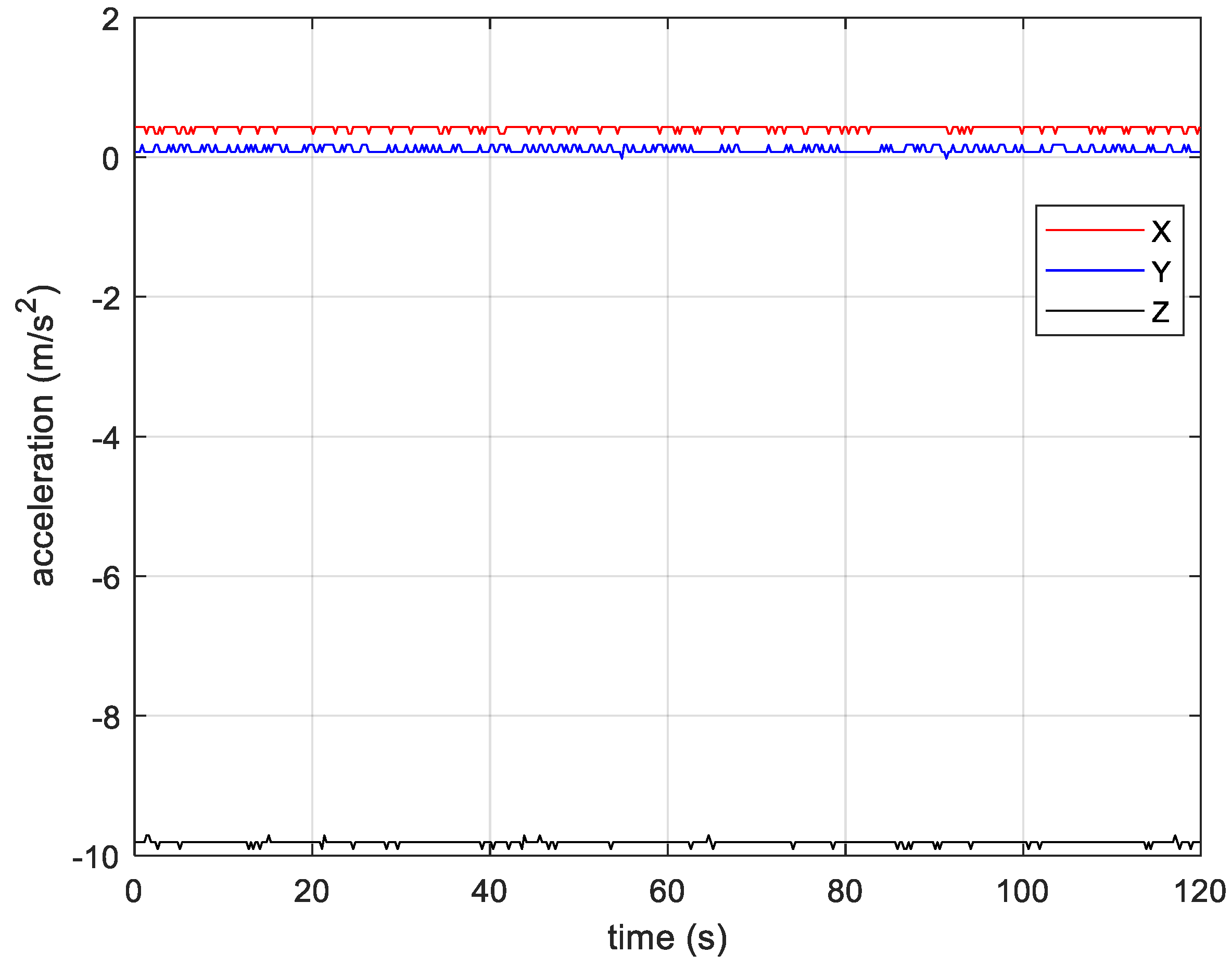
2.3. IMU and Accelerometer Calibration Procedure

The 10-DoF IMU sensor, produced by DFRobot, Inc. (Shangai, China) [37], integrates the ADXL345 accelerometer (Analog Devices, Norwood, MA, USA) [38], the HMC5883L magnetometer (Honeywell International, Inc., Plymouth, MN, USA) [39], the ITG-3205 triple-axis MEMS angular rate sensor (InvenSense, Inc., Sunnyvale, CA, USA) [40] and the BMP280 barometric pressure sensor (Bosch Sensortech GmbH, Reutligen, Germany) [41].

The relative position of the platform was estimated through the three components of the acceleration vector, by means of numerical double integration (integration of the velocity, i.e., of the integral of the acceleration) [42]. Figure 6 shows a sample of accelerometer data acquired by putting the sensor in a horizontal plane (x and y axes), therefore detecting gravity along the z axis.

The high sensitivity of acceleration measurements to platform vibrations, together with biases (offsets) or drifts, could give bad estimates of the double-integrated position. Other error sources are scale factor mismatch and misalignments between the accelerometer sensing axes and the platform body axes. The relationship between the raw measurements $a_x$, $a_y$ and $a_z$ and the actual acceleration components is modeled as:

$${\mathit{a}}_{\mathit{c}}={\mathit{A}}_m\left[\begin{array}{ccc}1/s_x& 0& 0\\ 0& 1/s_y& 0\\ 0& 0& 1/s_z\end{array}\right]\left[\begin{array}{c}{a}_x-o_x\\ a_y-o_y\\ a_z-o_z\end{array}\right]$$

(1)

where ${\mathit{a}}_c={\left(a_{cx},a_{cy},a_{cz}\right)}^{\mathit{T}}$, with T denoting transposition, is the actual acceleration vector (calibrated and normalized, i.e., $\sqrt{a_{cx}^2+a_{cy}^2+a_{cz}^2}=1$), ${\mathit{A}}_m$ is the 3 × 3 misalignment matrix, $s_x$, $s_y$ and $s_z$ are the scale factors, and $o_x$, $o_y$ and $o_z$ are the offsets. Equation (1) can be rearranged as:

$${\mathit{a}}_{\mathit{c}}=\left[\begin{array}{c}\begin{array}{ccc}{a}_{11}& a_{12}& a_{13}\\ a_{21}& a_{22}& a_{23}\end{array}\\ \begin{array}{ccc}{a}_{31}& a_{32}& a_{33}\end{array}\end{array}\right]\left[\begin{array}{c}{a}_x\\ a_y\\ a_z\end{array}\right]+\left[\begin{array}{c}{a}_1\\ a_2\\ a_3\end{array}\right]=\left[\begin{array}{c}{a}_{11}\\ a_{21}\\ a_{31}\end{array}\begin{array}{c}{a}_{12}\\ a_{22}\\ a_{32}\end{array}\begin{array}{c}{a}_{13}\\ a_{23}\\ a_{33}\end{array}\begin{array}{c}{a}_1\\ a_2\\ a_3\end{array}\right]\left[\begin{array}{c}\begin{array}{c}{a}_x\\ a_y\\ a_z\end{array}\\ 1\end{array}\right]$$

(2)

which is in the form ${\mathit{a}}_{\mathit{c}}=\mathit{X}·\mathit{u}$, with $\mathit{u}={\left[\begin{array}{ccc}{a}_x& a_y& a_{z}1\end{array}\right]}^{\mathit{T}}$. The 12 unknown calibration parameters are the elements of the matrix $\mathit{X}$. The least-squares solution gives for $\mathit{X}$ the following espression:

$$\mathit{X}={\mathit{a}}_{\mathit{c}}{\mathit{u}}^T{\left(\mathit{u}{\mathit{u}}^T\right)}^{-1}$$

(3)

To estimate the parameters involved in Equation (2), a calibration technique based on six stationary acquisitions [43] was implemented and run as an Arduino sketch. Setting two axes in a horizontal plane, the third axis was oriented in a +1 g and a −1 g field, minimizing the cross-axis sensitivity effect. We neglected changes in gravity due to changes in altitude and in latitude, and assumed for g the “local” value at a 45-degree latitude, $g_{45}=9.8066\mathrm{m}/{\mathrm{s}}^2$ [44]. As far as the ITG-3250 gyro is concerned, bias calibration (that is, zero output with stationary gyro) was performed using the standard functions (zeroCalibrate and getXYZ) included in the libraries hosted by the Arduino IDE (Integrated Development Environment) [45].

2.4. WiFi Module

To provide internet connectivity between the PODA platform and the PC-based ground station, the 3.3-V, 2.4-GHz Wi-Fi module ESP8266EX (Espressif Systems, Inc., Shangai, China) has been selected (Figure 7). This programmable, user friendly, low-cost module can work both as an access point and a station, fetching data from the microcontroller via an I²C interface, and uploading to the remote station, and can be used for a whole host of applications, from home automation to mobile devices, wearable electronics, Internet of Things (IoT) and Wi-Fi position system beacons. The module implements TCP/IP and full 802.11 b/g/n WLAN MAC protocol, with an average operating current of 80 mA, integrating antenna switches, a power amplifier and a low-noise receive amplifier, together with filters and power management subsystems. Interfacing with external sensors and other devices is achieved via on-chip SRAM (at least 512 kB) and a 32-bit RISC processor (L106 Diamond series, Tensilica Inc., San Jose, CA, USA) [46,47].

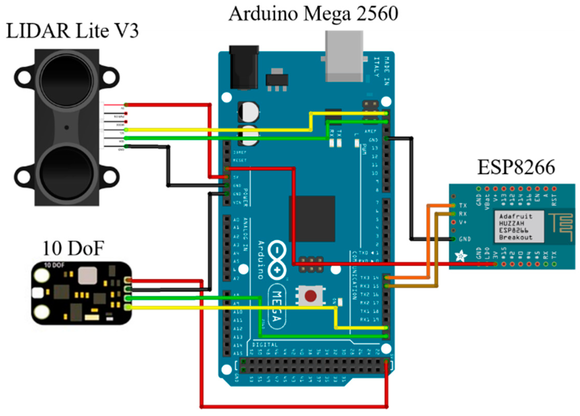
2.5. Microcontroller and Assembly

The Arduino Mega 2560 board acquires data from IMU and LiDAR, performs signal conditioning (a simple 1-D Kalman low-pass filtering for noise reduction of each acceleration component and of LiDAR measurements), and sends them to a PC laptop. Post-processing and mapping of the area that surrounds the UAV are performed in the Matlab^® environment. Figure 8 shows the data acquisition architecture: sensor data are gathered and managed through digital input pins, with standard I²C connection.

Data were transferred to the PC-based ground station via USB communication port during the laboratory tests with the prototype not installed on the drone, and via the ESP8266EX Wi-Fi module during the data acquisition campaigns. Figure 9 shows the PODA prototypical version mounted onboard the quadcopter.

Preliminary static tests were set up for accelerometer calibration, estimating the parameter matrix $\mathit{X}$ of Equation (3), and to determine measurement noise and accelerometer bias. The LiDAR measured distances along the z axis, whereas the x–y position and the velocity components were estimated through Kalman filtering of the accelerometer data, as explained below.

2.6. Platform State Estimation

A minimum-mean-square-error (MMSE) estimation of the six-element platform state vector $\mathit{x}={\left[x,y,z,v_x,v_y,v_z\right]}^T$ (position and velocity components) is implemented using Kalman filtering, typically described as an iterative prediction-updating-correction strategy [48]. Measurement noise $\mathit{\nu }$ and system process noise $\mathit{w}$ are assumed to be zero mean and Gaussian-distributed. The PODA platform is modeled as a discrete linear dynamic system:

$${\mathit{x}}_k={\mathit{A}}_k{\mathit{x}}_{k-1}+{\mathit{B}}_k{\mathit{u}}_{k-1}+{\mathit{w}}_{k-1}$$

(4)

where ${\mathit{x}}_k$ is the value of $\mathit{x}$ at time $t_k=k\Delta t$, ${\mathit{A}}_k$ the state transition matrix, containing the (generally time-dependent) coefficients of the state terms in the state dynamics, ${\mathit{B}}_k$ is the input matrix, relating the state to the inputs ${\mathit{u}}_{k-1}$, ${\mathit{w}}_k$ is the process noise vector, with zero mean and covariance matrix ${\mathit{Q}}_k$. The three calibrated and pre-filtered IMU-derived acceleration measurements ($\mathit{u}={\left[a_{cx},a_{cy},a_{cz}\right]}^T$) are modeled as inputs to the system. The measurement model is:

$${\mathit{z}}_k={\mathit{H}}_k{\mathit{x}}_k+{\mathit{\nu }}_k$$

(5)

where ${\mathit{z}}_k$ is the k^th measurement vector, ${\mathit{H}}_k$ is the observation matrix, and ${\mathit{\nu }}_k$ is the measurement noise vector, with zero mean and covariance matrix ${\mathit{R}}_k$, all of appropriate dimensions, and generally dependent on $t_k$.

The simple models used for the state transition matrix and the input matrix of Equation (4), and the observation matrix of Equation (5), are, respectively:

$$\mathit{A}=\left[\begin{array}{c}\begin{array}{ccc}\begin{array}{cc}1& 0\end{array}& \begin{array}{cc}0& \Delta t\end{array}& \begin{array}{cc}0& 0\end{array}\end{array}\\ \begin{array}{ccc}\begin{array}{cc}0& 1\end{array}& \begin{array}{cc}0& 0\end{array}& \begin{array}{cc}\Delta t& 0\end{array}\end{array}\\ \begin{array}{ccc}\begin{array}{cc}0& 0\end{array}& \begin{array}{cc}1& 0\end{array}& \begin{array}{cc}0& \Delta t\end{array}\end{array}\\ \begin{array}{ccc}\begin{array}{cc}0& 0\end{array}& \begin{array}{cc}0& 1\end{array}& \begin{array}{cc}0& 0\end{array}\end{array}\\ \begin{array}{ccc}\begin{array}{cc}0& 0\end{array}& \begin{array}{cc}0& 0\end{array}& \begin{array}{cc}1& 0\end{array}\end{array}\\ \begin{array}{ccc}\begin{array}{cc}0& 0\end{array}& \begin{array}{cc}0& 0\end{array}& \begin{array}{cc}0& 1\end{array}\end{array}\end{array}\right],\mathit{B}=\left[\begin{array}{c}\begin{array}{ccc}\frac{1}{2}\Delta t^2& 0& 0\end{array}\\ \begin{array}{ccc}0& \frac{1}{2}\Delta t^2& 0\end{array}\\ \begin{array}{ccc}0& 0& \frac{1}{2}\Delta t^2\end{array}\\ \begin{array}{ccc}\Delta t& 0& 0\end{array}\\ \begin{array}{ccc}0& \Delta t& 0\end{array}\\ \begin{array}{ccc}0& 0& \Delta t\end{array}\end{array}\right],\mathit{H}=\left[\begin{array}{c}\begin{array}{ccc}\begin{array}{cc}0& 0\end{array}& \begin{array}{cc}0& \Delta t^{-1}\end{array}& \begin{array}{cc}0& 0\end{array}\end{array}\\ \begin{array}{ccc}\begin{array}{cc}0& 0\end{array}& \begin{array}{cc}0& 0\end{array}& \begin{array}{cc}\Delta t^{-1}& 0\end{array}\end{array}\\ \begin{array}{ccc}\begin{array}{cc}0& 0\end{array}& \begin{array}{cc}0& 0\end{array}& \begin{array}{cc}0& \Delta t^{-1}\end{array}\end{array}\end{array}\right]$$

(6)

where $\Delta t$ is the sampling time. The predictor stage is as follows:

$${\widehat{\mathit{x}}}_{k|k-1}={\mathit{A}}_k{\widehat{\mathit{x}}}_{k-1}+\mathit{B}{\mathit{u}}_{\mathit{k}}$$

(7)

$${\mathit{P}}_{k|k-1}=\mathit{A}{\mathit{P}}_{k-1}{\mathit{A}}^T+\mathit{Q}$$

(8)

In Equation (7), ${\widehat{\mathit{x}}}_{k|k-1}$ is the predicted state (i.e., the state at discrete time $t_k$), given the previous state ${\widehat{\mathit{x}}}_{k-1}$, evaluated at time $t_{k-1}$. For simplicity, the $6\times 6$ matrix ${\mathit{Q}}_k$ has been set to 0,$\forall k$ (no process noise). Equation (8) predicts the state error covariance matrix ${\mathit{P}}_{k|k-1}$ at $t_k$, which allows us to calculate the Kalman gain:

$${\mathit{K}}_k={\mathit{P}}_{k|k-1}{\mathit{H}}^T{\left(\mathit{H}{\mathit{P}}_{k|k-1}{\mathit{H}}^T+\mathit{R}\right)}^{-1}$$

(9)

In the corrector stage, the new estimate is updated from the current measurement, the old estimate and the value of ${\mathit{K}}_k$:

$${\widehat{\mathit{x}}}_k={\widehat{\mathit{x}}}_{k|k-1}+{\mathit{K}}_k\left({\mathit{z}}_k-\mathit{H}{\widehat{\mathit{x}}}_{k|k-1}\right)$$

(10)

where ${\mathit{z}}_k-\mathit{H}{\widehat{\mathit{x}}}_{k|k-1}$ is the innovation, i.e., the measurement pre-fit residual. The state error covariance is updated as follows:

$${\mathit{P}}_k=\left(\mathit{I}-{\mathit{K}}_k\mathit{H}\right){\mathit{P}}_{k|k-1}$$

(11)

where I is the $6\times 6$ identity matrix. The value of ${\mathit{R}}_k$, estimated from static and dynamic test measurements (see

Table 1. Variances of raw and filtered LiDAR and IMU data (x- and y-components of accelerations, and double-integrated z-component, fused with LiDAR data).

Distance (cm)	LiDAR		LiDAR+IMU Fusion		${\mathit{a}}_{\mathit{x}},{\mathit{a}}_{\mathit{y}}\left(\mathbf{IMU}\right)$
	${\mathit{\sigma }}_{\mathit{L},\mathit{r}\mathit{a}\mathit{w}}^2$	${\mathit{\sigma }}_{\mathit{L},\mathit{f}}^2$	${\mathit{\sigma }}_{\mathit{r}\mathit{a}\mathit{w}}^2$	${\mathit{\sigma }}_{\mathit{f}}^2$	${\mathit{\sigma }}_{\mathit{a},\mathit{r}\mathit{a}\mathit{w}}^2$	${\mathit{\sigma }}_{\mathit{a},\mathit{f}}^2$
	(cm2)	(cm2)	(cm2)	(cm2)	(m2/s4)	(m2/s4)
120	1.69	1.00	1.00	0.40	0.80	0.32
90	0.755	0.40	0.50	0.30	0.57	0.36
30	10.4	1.64	0.40	0.28	0.34	0.26

), and assumed constant, has been found to be:

$${\mathit{R}}_k=\mathit{R}=\left[\begin{array}{ccc}{\sigma }_{a_x}^2& 0& 0\\ 0& {\sigma }_{a_y}^2& 0\\ 0& 0& {\sigma }_{a_z}^2\end{array}\right]=\left[\begin{array}{ccc}0.80& 0& 0\\ 0& 0.80& 0\\ 0& 0& 0.80\end{array}\right]\frac{m^2}{s^4}$$

(12)

The KF, implemented in the Arduino IDE, ran in real-time during the data acquisition sessions, using as input the x-, y- and z-components of ${\mathit{a}}_c$. Post-processed numerical double integration of the pre-filtered calibrated acceleration components gave the platform position in the xyz plane, which was in good agreement with the real-time KF-derived position.

3. Experimental Results and System Validation

During the experimental sessions (drone equipped with PODA), data were collected in 2-min acquisitions at 10-Hz sampling frequency (i.e., a measurement each $\Delta t=0.1\mathrm{s}$, 1200 samples per experiment). A first validation of the PODA system was performed by installing the platform on the drone and acquiring data during a 2-min landing procedure from a height of 150 cm (initial position [0 cm, 0 cm, 150 cm]) above ground level, hovering for about 20 s at five intermediate stations (120 cm, 90 cm, 60 cm and 30 cm). The LiDAR pointed towards the ground and gathered vertical distances, whereas the landing point was located at [100 cm, 50 cm, 0 cm]. The distance between the starting and the landing points was 190 cm.

The 10-DoF IMU collected x–y positioning data (by double integration of $a_x$ and $a_y$, after removing bias and measurement noise) and attitude (roll and pitch angles, by integration of the rate gyros measurements, after removing bias and drift). Double integration of the z-component of the acceleration was used for comparison and fusion with the distance data acquired by LiDAR, to attain an estimate $\widehat{z}$ of the z position during the descent. A simple data fusion technique [49], assuming the optimal (minimum-variance) estimate $\widehat{z}$ as a linear function of the LiDAR data ($z_L)$ and double-integrated accelerometer measurements ($z_{acc})$, with variances ${\sigma }_L^2$ and ${\sigma }_{acc}^2$, respectively, was implemented to get $\widehat{z}$:

$$\widehat{z}=\left(\frac{{\sigma }_{acc}^2}{{\sigma }_{acc}^2+{\sigma }_L^2}\right)z_L+\left(\frac{{\sigma }_L^2}{{\sigma }_{acc}^2+{\sigma }_L^2}\right)z_{acc}=z_L+\frac{{\sigma }_L^2}{{\sigma }_{acc}^2+{\sigma }_L^2}\left(z_{acc}-z_L\right)$$

(13)

The rightmost expression of Equation (13) shows that the data fusion methodology is equivalent to a simple 1-D KF with $\mathit{H}$=1, $\mathit{R}={\sigma }_{acc}^2$, $\mathit{P}=1$, $z_{acc}$ being the measurement and $z_L$ being the “state”. Figure 10a shows LiDAR-derived distances (raw and filtered measurements) during the indoor landing simulation, with 20 s of hovering at the six stations previously mentioned, and a descent of 2 s to the successive station. In Figure 10b the attitude history (pitch and roll angles), recorded by the calibrated IMU’s rate gyro, is shown.

Figure 11a,b show the raw and filtered x- and y-components of the measured acceleration, respectively. The high-frequency components have been attenuated by the prefiltering.

A small offset (in the order of ±0.2 m/s²), due to small misalignment errors, is noticeable on both $a_x$ and $a_y$. The offline calibration procedure previously described (Section 2.3) allowed us to compensate for this bias and remove drift in the double integration procedure. Figure 12 compares the true landing path to the path obtained from raw LiDAR and IMU data, and from filtered observations. The estimated trajectory (filtered data) show a reduction of the drift in the x and y positions due to the double-integrated acceleration measurements (“Raw data” in the figure). The z position has been obtained by data fusion (Equation (13)).

Ground truth data, necessary for assessing the quality of the estimated trajectory, were collected by measuring, during each hovering interval (approximately 20 s), the distance from the ground and the xyz position with a laser range finder (Sndway^® ST-100, ±2-mm accuracy, built by Dongguan Senwey Electronic Co., Guangdong, China). The five measured stations are indicated by circles on the “Real data” trajectory.

The PODA platform was successively tested in indoor and outdoor data acquisition campaigns. Figure 13 shows raw and estimated platform positions during a takeoff (data acquisition began at zero-height), followed by a climb up to 150 cm. In Figure 14, a complete flight (3 min) with random maneuvers is shown, with data acquired and downlinked to the ground station just after the takeoff and up to few seconds before landing. Figure 15 shows data acquired during a landing phase, from 150 cm to zero-height.

Finally, a GVI mission was simulated, using the PODA system onboard the drone during three indoor flights around an aluminum plate (dimensions 1300 mm × 1500 mm × 3 mm), located at a 400-mm height. Results are plotted in Figure 16.

Table 1 shows measurement uncertainties evaluated at three hovering stations of the simulated landing (120 cm, 90 cm and 30 cm, respectively). Variances of raw and filtered LiDAR measurements, LiDAR-IMU distance from the ground and acceleration components ($a_x$, $a_y$) are reported. The filtered data show up to 55% improved accuracy. For example, the variance of the LiDAR-derived distance at 120 cm decreased from 1.69 cm² (before filtering) to 1.00 cm² after filtering. The data fusion strategy adopted for height estimation gives even better accuracy (from 1.00 cm² to 0.40 cm², 60% improvement).

4. Conclusions and Future Work

The main objective of this investigation is the development and validation of an embedded system for a Positioning, field mapping, Obstacle Detection and Avoidance system (PODA) for a UAV. Lightweight, low-cost sensors (LiDAR and 10-DoF IMU), a Wi-Fi module for data downlink to a ground station (PC or tablet) and a programmable microcontroller (Arduino Mega 2560) with standard I²C interface are the main components of the PODA platform, which has shown adaptability, sustainability and cost reduction. The platform is tailored to fit different aerial vehicles, and its functionality is suitable to different applications that require positioning, field mapping and obstacle detection. The sensors’ calibration procedure and the platform’s state estimation technique have been described, together with a real-time pre-filtering (signal conditioning) technique for measurement noise mitigation. A simple data fusion methodology has been applied to the distance from the ground measured by the LiDAR and the altitude derived by double integration of the vertical component of the acceleration. The algorithms were tested in both hardware-in-the-loop simulations and on an actual UAV. Experimental results from indoor and outdoor campaigns and different scenarios (landing and inspection flights) with the PODA platform onboard a commercial quadrotor (Parrot Ar.Drone 2.0) have shown that double integration of the calibrated acceleration data, fused with raw LiDAR measurements, reduces uncertainties to the centimetre level. This feature can be effective for maneuvering the drone in critical conditions, detecting obstacles or intruders, and use during precise hovering and landing procedures. As expected, the Kalman-based estimation of the platform state vector significantly reduces the uncertainties regarding the vehicle’s position and trajectory.

Future research activity will focus on developing fully automatic obstacle detection within the capabilities of the PODA system, and on analyzing the influence of changes in angle to the target (i.e., platform attitude) on the accuracy of LiDAR distance measurements. More complex indoor and outdoor conditions will allow us to validate the algorithms in different scenarios, and to explore the influence of different external factors on system performance. In order to design controllers and implement a DAA strategy, which is one of the functionalities foreseen for the PODA system, a Simulink model of the quadcopter dynamics is currently being developed. Further capabilities of the PODA platform, such as object and/or pattern recognition for safe landing area identification, are being studied for future conceptual improvements, focusing on strategies that would require little computational effort and a minimal amount of hardware. A promising approach could be a “learned sensing” strategy, relying on machine learning techniques [50]. Multisensor data fusion could also be improved by using methodologies that are useful in the context of non-Gaussian conditions, and unknown or complicated cross-correlations between sensors, such as the arithmetical average (AA) fusion rule [51,52]. Finally, improved estimation techniques, such as extended KF to account for nonlinearities, unscented KF or particle filtering, will be tested for there capacity to give autonomous flight and collision avoidance capability, with a reliable and cheap sensor suite, while still keeping the computational cost low, and reducing maintenance and development costs.

References

1. Valavanis, K.V. Advances in Unmanned Aerial Vehicles—State of Art and the Road to Autonomy; Springer: Berlin/Heidelberg, Germany, 2007. [Google Scholar]
2. Papa, U. Embedded Platforms for UAS Landing Path and Obstacle Detection: Integration and Development of Unmanned Aircraft Systems; Springer: Berlin/Heidelberg, Germany, 2018; Volume 136. [Google Scholar]
3. Lillian, B. FAA Predicts Future UAS Growth. 2019. Available online: https://unmanned-aerial.com/faa-predicts-future-uas-growth (accessed on 15 May 2020).
4. González-Jorge, H.; Martínez-Sánchez, J.; Bueno, M.; Arias, P. Unmanned Aerial Systems for Civil Applications: A Review. Drones 2017, 1, 2. [Google Scholar] [CrossRef]
5. Sigala, A.; Langhals, B. Applications of Unmanned Aerial Systems (UAS): A Delphi Study Projecting Future UAS Missions and Relevant Challenges. Drones 2020, 4, 8. [Google Scholar] [CrossRef] [Green Version]
6. Dept. of Transportation. Unmanned Aircraft Systems (UAS) Service Demand 2015-2035: Literature Review & Projections of Future Usage; Technical Report, Version 0.1; UASF Aerospace Management Systems Division, Air Traffic Systems Branch (AFLCMC/HBAG): Bedford, MA, USA, 2013; 151p. [Google Scholar]
7. Ollero, A. UAV Applications. In Handbook of Unmanned Aerial Vehicles; Valavanis, K.P., Vachtsevanos, G.J., Eds.; Springer: Berlin/Heidelberg, Germany, 2015; pp. 2638–2860. [Google Scholar]
8. MahmoudZadeh, S.; Powers, D.M.W.; Zadeh, R.B. Autonomy and Unmanned Vehicles—Augmented Reactive Mission and Motion Planning Architecture; Springer Nature Singapore Pte Ltd.: Singapore, 2019; 66C-PRT; Volume I, pp. 562–566. [Google Scholar]
9. Mustapha, B.; Zayegh, A.; Begg, R.K. Multiple sensors based obstacle detection system. In Proceedings of the 4th International Conference on Intelligent and Advanced Systems (ICIAS2012), Kuala Lumpur, Malaysia, 12–14 June 2012. [Google Scholar]
10. Gageik, N.; Benz, P.; Montenegro, S. Obstacle Detection and Collision Avoidance for a UAV with Complementary Low-Cost Sensors. IEEE Access 2015, 3, 599–609. [Google Scholar] [CrossRef]
11. Engel, J.; Sturm, J.; Cremers, D. Camera-based navigation of a low-cost quadrocopter. In Proceedings of the 2012 IEEE/RSJ International Conference on Intelligent Robots and Systems, Vilamoura, Portugal, 7–12 October 2012; pp. 2815–2821. [Google Scholar] [CrossRef] [Green Version]
12. Aswini, N.; Uma, S.V. Obstacle Detection in Drones Using Computer Vision Algorithm. In Advances in Signal Processing and Intelligent Recognition Systems. SIRS 2018; Thampi, S., Marques, O., Krishnan, S., Li, K.C., Ciuonzo, D., Kolekar, M., Eds.; Communications in Computer and Information Science; Springer: Singapore, 2019; Volume 968. [Google Scholar]
13. Phan, C.; Liu, H.H. A cooperative UAV/UGV platform for wildfire detection and fighting. In Proceedings of the 2008 Asia Simulation Conference–7th International Conference on System Simulation and Scientific Computing, Beijing, China, 10–12 December 2008; pp. 494–498. [Google Scholar]
14. Austin, R. Unmanned Aircraft Systems: UAVS Design, Development and Deployment; Wiley and Sons, Ltd.: Hoboken, NJ, USA, 2010. [Google Scholar]
15. Kendoul, F. Survey of advances in guidance, navigation, and control of unmanned rotorcraft systems. J. Field Robot. 2012, 29, 315–378. [Google Scholar] [CrossRef]
16. Sobers, D.M.; Chowdhary, G., Jr.; Johnson, E.N. Indoor Navigation for Unmanned Aerial Vehicles. In Proceedings of the AIAA Guidance, Navigation, and Control Conference, Chicago, IL, USA, 10–13 August 2009. [Google Scholar]
17. Fraga-Lamas, P.; Ramos, L.; Mondéjar-Guerra, V.; Fernández-Caramés, T.M. A Review on IoT Deep Learning UAV Systems for Autonomous Obstacle Detection and Collision Avoidance. Remote. Sens. 2019, 11, 2144. [Google Scholar] [CrossRef] [Green Version]
18. Papa, U.; Del Core, G. Design and Assembling of a Low-Cost Mini UAV Quadcopter System; Technical Paper; Department of Science and Technology, University of Naples “Parthenope”: Napoli, Italy, 2014. [Google Scholar]
19. Ariante, G.; Papa, U.; Ponte, S.; Del Core, G. UAS for positioning and field mapping using LiDAR and IMU sensors data: Kalman filtering and integration. In Proceedings of the 2019 IEEE 5th International Workshop on Metrology for AeroSpace, Torino, Italy, 19–21 June 2019; pp. 522–527. [Google Scholar] [CrossRef]
20. Ariante, G. Embedded System for Precision Positioning, Detection, and Avoidance (PODA) for Small UAS. IEEE A&E Syst. Mag. 2020. in print. [Google Scholar] [CrossRef]
21. Scherer, S.; Chamberlain, L.; Singh, S. Autonomous landing at unprepared sites by a full-scale helicopter. Robot. Auton. Syst. 2012, 60, 1545–1562. [Google Scholar] [CrossRef]
22. Jeong, N.; Hwang, H.; Matson, E.T. Evaluation of low-cost LiDAR sensor for application in indoor UAV navigation. In Proceedings of the 2018 IEEE Sensors Applications Symposium (SAS), Seoul, Korea, 12–14 March 2018; pp. 1–5. [Google Scholar] [CrossRef]
23. Gui, P.; Tang, L.; Mukhopadhyay, S. MEMS based IMU for tilting measurement: Comparison of complementary and kalman filter based data fusion. In Proceedings of the 2015 IEEE 10th Conference on Industrial Electronics and Applications (ICIEA), Auckland, New Zealand, 15–17 June 2015; pp. 2004–2009. [Google Scholar]
24. McCarron, B. Low-Cost IMU Implementation via Sensor Fusion Algorithms in the Arduino Environment; Polytechnic State University: San Obispo, CA, USA, 2013. [Google Scholar]
25. Kumar, G.A.; Patil, A.K.; Patil, R.; Park, S.S.; Chai, Y.H. A LiDAR and IMU Integrated Indoor Navigation System for UAV and Its Application in Real-Time Pipeline Classification. Sensors 2017, 17, 1268. [Google Scholar] [CrossRef] [PubMed] [Green Version]
26. Papa, U.; Ariante, G.; Del Core, G. UAS Aided Landing and Obstacle Detection through LiDAR-Sonar data. In Proceedings of the 2018 5th IEEE International Workshop on Metrology for AeroSpace, Rome, Italy, 20–22 June 2018. [Google Scholar]
27. Papa, U.; Del Core, G. Design of sonar sensor model for safe landing of UAVs. In Proceedings of the IEEE Workshop on Metrology for Aerospace, Benevento, Italy, 4–5 June 2015; pp. 361–365. [Google Scholar]
28. Papa, U.; Ponte, S. Preliminary Design of an Unmanned Aircraft System for Aircraft General Visual Inspection. Electronics 2018, 7, 435. [Google Scholar] [CrossRef] [Green Version]
29. Son, J.-H.; Choi, S.; Cha, J. A brief survey of sensors for detect, sense, and avoid operations of Small Unmanned Aerial Vehicles. In Proceedings of the 2017 17th International Conference on Control, Automation and Systems (ICCAS), Jeju, Korea, 18–21 October 2017; pp. 279–282. [Google Scholar]
30. Gautam, A.; Sujit, P.; Saripalli, S. A survey of autonomous landing techniques for UAVs. In Proceedings of the 2014 International Conference on Unmanned Aircraft Systems, ICUAS 2014—Conference Proceedings, Orlando, FL, USA, 27–30 May 2014; pp. 1210–1218. [Google Scholar]
31. Krajnìk, T.; Vonàsek, V.; Fišer, D.; Faigl, J. AR-Drone as a Platform for Robotic Research and Education. In EUROBOT 2011, CCIS 161; Obdržálek, D., Gottscheber, A., Eds.; Springer: Berlin/Heidelberg, Germany, 2011; pp. 172–186. [Google Scholar]
32. Mac, T.T.; Copot, C.; Ionescu, C.M. Detection and Estimation of Moving obstacles for a UAV. IFAC-PapersOnLine 2019, 52, 22–27. [Google Scholar] [CrossRef]
33. Parrot Drones SAS. Parrot AR. Drone 2.0 Elite Edition—Description and Technical Data. 2019. Available online: https://www.parrot.com/eu/drones/parrot-ardrone-20-elite-edition#parrot-ardrone-20-elite-edition (accessed on 10 January 2020).
34. Garmin. Lidar.Lite v3 Operation Manual and Technical Specifications; Garmin Ltd.: Olathe, KS, USA, 2016; Available online: https://static.garmin.com/pumac/LiDAR_Lite_v3_Operation_Manual_and_Technical_Specifications.pdf (accessed on 10 March 2020).
35. I2C Info. I2C Info—I2C Bus, Interface and Protocol. 2020. Available online: https://i2c.info/ (accessed on 15 April 2020).
36. Meier, R. Roger Meier’s Freeware. 2020. Available online: https://freeware.the-meiers.org/ (accessed on 15 April 2020).
37. DFRobot. 10- DoF MEMS IMU Sensor V2.0 2020. Available online: https://www.dfrobot.com/wiki/index.php/10_DOF_Mems_IMU_Sensor_V2.0_SKU:_SEN0140 (accessed on 20 March 2020).
38. Analog Devices. Small, Low Power, 3-Axis ±3g Accelerometer ADXL335-345—Rev. 0 2009. Available online: https://www.sparkfun.com/datasheets/Components/SMD/adxl335.pdf (accessed on 10 March 2020).
39. Honeywell Inc. 3-Axis Digital Compass IC HMC5883L—Advanced Information. 2013. Available online: https://www.jameco.com/Jameco/Products/ProdDS/2150248.pdf (accessed on 20 February 2020).
40. InvenSense Inc. ITG-3205 Product Specification—Revision 1.0. Document Number: PS-ITG-3205A-00. 2010. Available online: https://www.tinyosshop.com/datasheet/itg3205.pdf (accessed on 10 May 2020).
41. Bosch Sensortec. BMP280 Digital Pressure Sensor Datasheet; Rev. 1.13, BST-BMP280-DS001-10; Bosch Sensortec GmbH: Reutlingen, Germany, 2014. [Google Scholar]
42. Thong, Y.; Woolfson, M.; Crowe, J.; Hayes-Gill, B.; Jones, D. Numerical double integration of acceleration measurements in noise. Measurement 2004, 36, 73–92. [Google Scholar] [CrossRef]
43. ST Microelectronics. Application Note AN4508—Parameters and Calibration of a Low-g 3-Axis Accelerometer; DocID026444-Rev 1; ST Microelectronics: Geneva, Switzerland, 2014; 13p, Available online: https://html.alldatasheet.vn/html-pdf/694488/STMICROELECTRONICS/AN4508/1943/1/AN4508.html (accessed on 17 July 2020).
44. Stevens, B.L.; Lewis, F.L.; Johnson, E.N. Aircraft Control and Simulation (3rd Edition)—Dynamics, Controls Design, and Autonomous Systems; John Wiley & Sons Inc.: Hoboken, NJ, USA, 2016. [Google Scholar]
45. Seed Studio. Arduino Library to Control Grove 3-Axis Digital Gyro Base on ITG 3200. 2013. Available online: https://github.com/Seeed-Studio/Grove_3_Axis_Digital_Gyro (accessed on 3 June 2020).
46. Espressif Systems IOT Team. ESP8266EX Datasheet—Version 4.3. 2015. Available online: https://www.espressif.com/sites/default/files/documentation/0a-esp8266ex_datasheet_en.pdf (accessed on 20 April 2020).
47. Espressif Systems IOT Team. ESP8266EX Technical Reference—Version 1.4. 2019. Available online: https://www.espressif.com/sites/default/files/documentation/esp8266-technical_reference_en.pdf (accessed on 20 April 2020).
48. Grewal, M.; Andrews, A. Kalman Filtering—Theory and Practice Using MATLAB®, 4th ed.; John Wiley & Sons, Inc.: Hoboken, NJ, USA, 2015. [Google Scholar]
49. Gelb, A. (Ed.) Applied Optimal Estimation; MIT Press: Cambridge, MA, USA; London, UK, 1974; p. 2001. [Google Scholar]
50. Del Hougne, P.; Imani, M.F.; Diebold, A.V.; Horstmeyer, R.; Smith, D.R. Learned Integrated Sensing Pipeline: Reconfigurable Metasurface Transceivers as Trainable Physical Layer in an Artificial Neural Network. Adv. Sci. 2019, 7, 1901913. [Google Scholar] [CrossRef] [PubMed] [Green Version]
51. Li, T.; Corchado, J.M.; Bajo, J.; Sun, S.; De Paz, J.F. Effectiveness of Bayesian filters: An information fusion perspective. Inf. Sci. 2016, 329, 670–689. [Google Scholar] [CrossRef]
52. Li, T.; Wang, X.; Liang, Y.; Pan, Q. On Arithmetic Average Fusion and Its Application for Distributed Multi-Bernoulli Multitarget Tracking. IEEE Trans. Signal Process. 2020, 1. [Google Scholar] [CrossRef]
Figure 1. Conceptual block diagram of the Positioning, field mapping, Obstacle Detection and Avoiding (PODA) subsystem.
Electronics 09 01175 g001
Figure 2. Parrot AR.Drone 2.0 and coordinate system.
Electronics 09 01175 g002
Figure 3. (a) Garmin LiDAR-Lite v3 (size 20 × 48 × 40 mm, weight 22 g). (b) Example of distance measurement in static conditions (nominal distance between sensor and obstacle: 50 cm).
Electronics 09 01175 g003
Figure 4. LiDAR distance measurements after bias removal. Each dot represents the average of 480 measurements at a sampling frequency of 4 Hz, i.e., 120-s acquisition time per distance value.
Electronics 09 01175 g004
Figure 5. Variances of raw LiDAR distance measurements (5-cm steps from 30 cm to 180 cm).
Electronics 09 01175 g005
Figure 6. Raw accelerometer data (static test, no filtering). The nonzero x- and y-components are due to non-optimal alignment between the accelerometer axes and the body reference system.
Electronics 09 01175 g006
Figure 7. Espressif Systems Wi-Fi module ESP8266EX and pinout.
Electronics 09 01175 g007
Figure 8. Electrical interface of the data acquisition and Wi-Fi communication system.
Electronics 09 01175 g008
Figure 9. PODA platform (prototypical version) mounted onboard the quadcopter. Each square of the ruler on the left side of the image has 1-cm side length.
Electronics 09 01175 g009
Figure 10. (a) Landing with intermediate hovering stations: raw and filtered LiDAR distances from the ground. (b) Raw and filtered calibrated attitude data (pitch and roll).
Electronics 09 01175 g010aElectronics 09 01175 g010b
Figure 11. (a) Raw and filtered x-component of the acceleration. (b) y-component of the acceleration.
Electronics 09 01175 g011aElectronics 09 01175 g011b
Figure 12. Comparison between estimated (KF) and measured (raw data) landing paths.
Electronics 09 01175 g012
Figure 13. Takeoff and climb to a 150-cm height: raw data and KF-based position estimation.
Electronics 09 01175 g013
Figure 14. A 3-min flight with random maneuvers.
Electronics 09 01175 g014
Figure 15. Landing from a 150-cm height to ground.
Electronics 09 01175 g015
Figure 16. (a) PODA trajectory acquisition. (b) General Visual Inspection (GVI) application: flights around an aluminum plate.
Electronics 09 01175 g016