Electric Field Evaluation Using the Finite Element Method and Proxy Models for the Design of Stator Slots in a Permanent Magnet Synchronous Motor

 ,
,  , , , and
Abstract
:1. Introduction
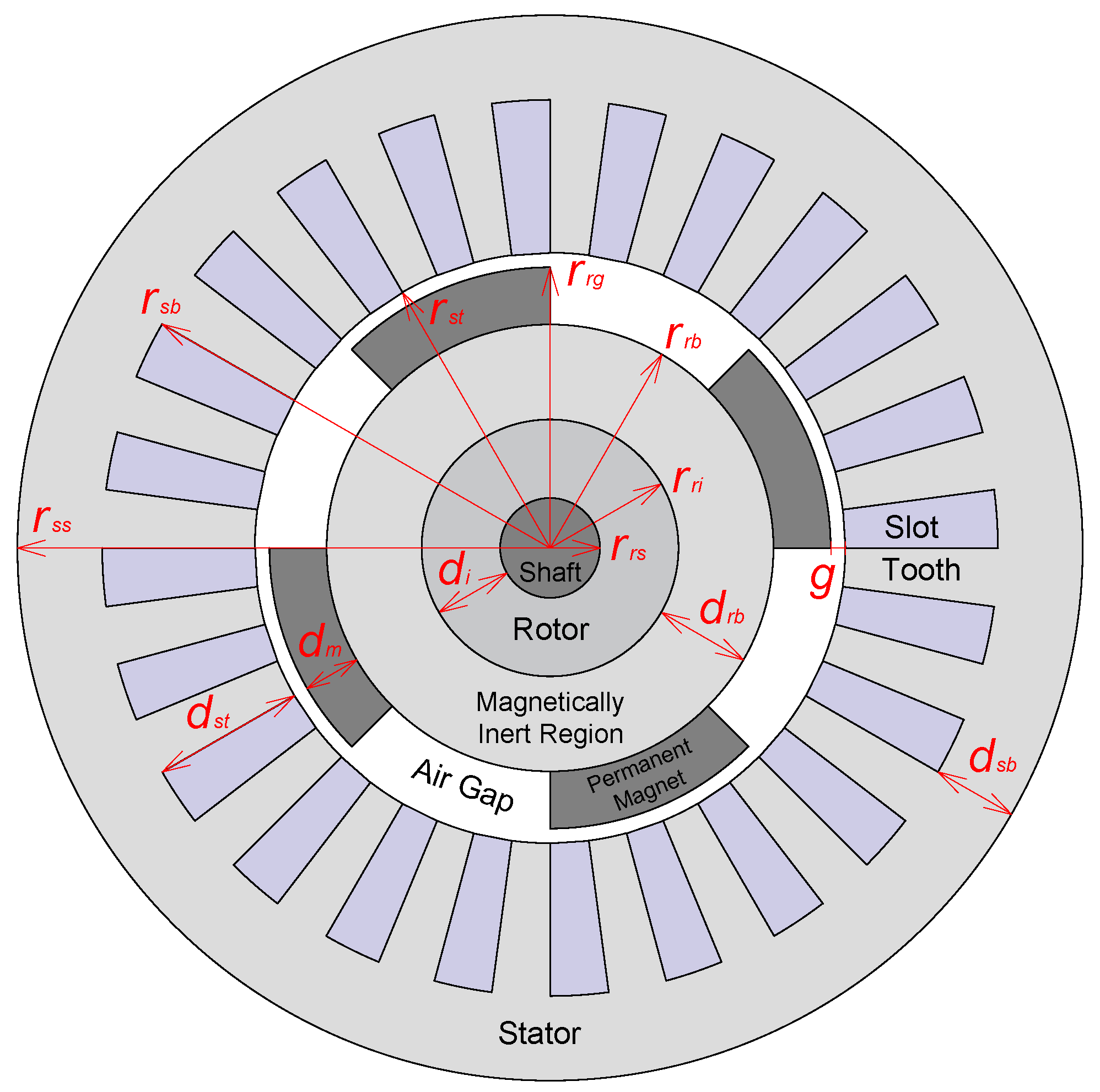
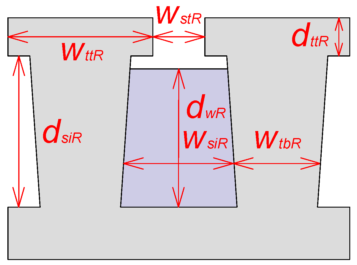
2. Machine Geometry
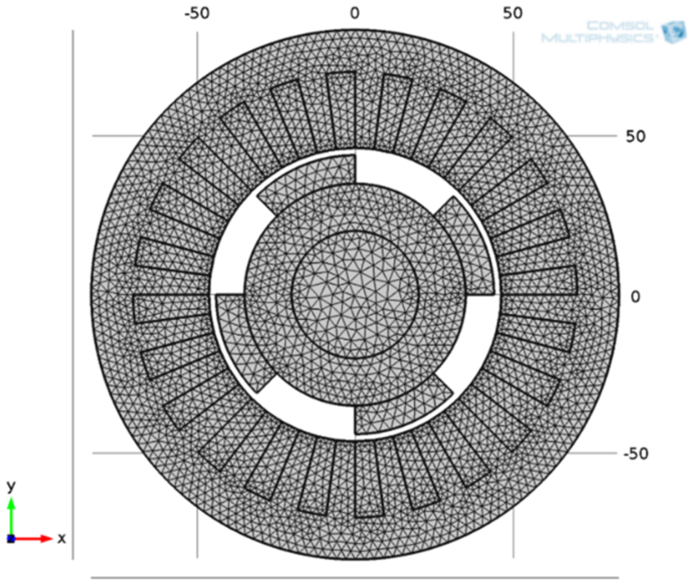
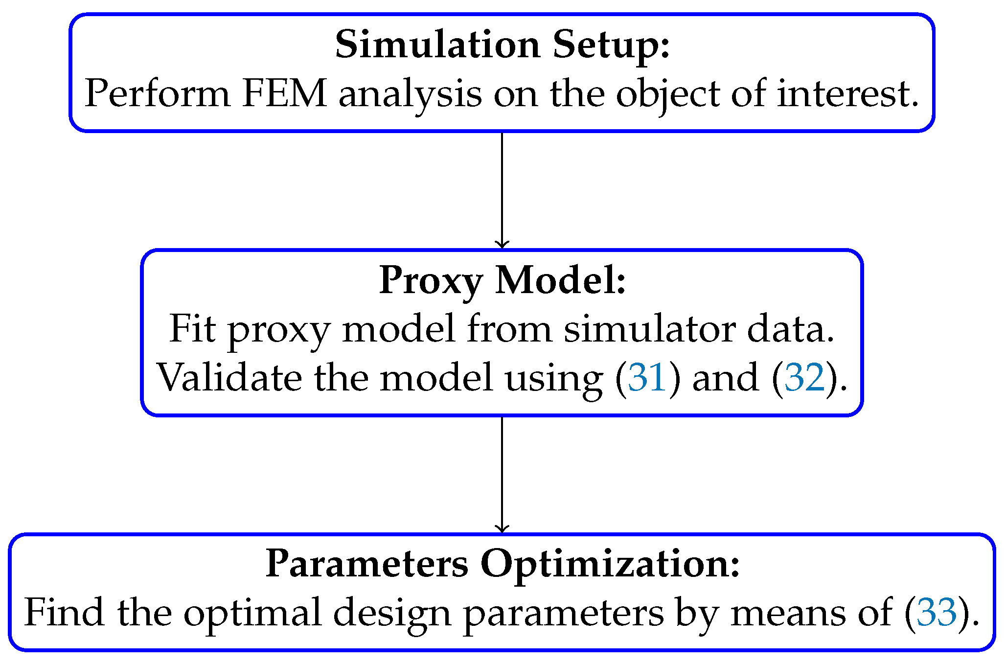
3. Optimized Finite Element Method
3.1. FEM Elements Calculation
3.2. Parameter Optimization
4. Analysis of the Proposed Methodology
4.1. Optimized Finite Element Method
4.1.1. Polynomial Regression
4.1.2. Neural Network
4.1.3. Discussion
5. Conclusions
Author Contributions
Funding
Acknowledgments
Conflicts of Interest
Abbreviations
| CAPES | Coordination of Superior Level Staff Improvement |
| DFO | Derivative-Free Optimization |
| FEM | Finite Element Method |
| IPOPT | Interior Point OPTimizer |
| MADS | Mesh Adaptive Direct Search |
| MILP | Mixed-integer linear problem |
| MSE | Mean Squared Error |
| NLP | Nonlinear Problem |
| NOMAD | Nonlinear Optimization with the MADS Algorithm |
| PMSM | Permanent Magnet Synchronous Machine |
| PSO | Particle Swarm Optimization |
| ReLU | Rectified Linear Unit |
| SSR | Sum of Squared Residuals |
| SST | Sum of Squares Total |
References
- Stefenon, S.F.; Branco, N.W.; Nied, A.; Bertol, D.W.; Finardi, E.C.; Sartori, A.; Meyer, L.H.; Grebogi, R.B. Analysis of training techniques of ANN for classification of insulators in electrical power systems. IET Gener. Transm. Distrib. 2020, 14, 1591–1597. [Google Scholar] [CrossRef]
- Ribeiro, M.H.D.M.; Stefenon, S.F.; de Lima, J.D.; Nied, A.; Marini, V.C.; de Coelho, L.S. Electricity Price Forecasting Based on Self-Adaptive Decomposition and Heterogeneous Ensemble Learning. Energies 2020, 13, 5190. [Google Scholar] [CrossRef]
- Stefenon, S.F.; Silva, M.C.; Bertol, D.W.; Meyer, L.H.; Nied, A. Fault diagnosis of insulators from ultrasound detection using neural networks. J. Intell. Fuzzy Syst. 2019, 37, 6655–6664. [Google Scholar] [CrossRef]
- Feng, G.; Lai, C.; Kar, N.C. Practical testing solutions to optimal stator harmonic current design for PMSM torque ripple minimization using speed harmonics. IEEE Trans. Power Electron. 2017, 33, 5181–5191. [Google Scholar] [CrossRef]
- Stefenon, S.F.; Americo, J.P.; Meyer, L.H.; Grebogi, R.B.; Nied, A. Analysis of the electric field in porcelain pin-type insulators via finite elements software. IEEE Lat. Am. Trans. 2018, 16, 2505–2512. [Google Scholar] [CrossRef]
- Corso, M.P.; Stefenon, S.F.; Couto, V.F.; Cabral, S.H.L.; Nied, A. Evaluation of methods for electric field calculation in transmission lines. IEEE Lat. Am. Trans. 2018, 16, 2970–2976. [Google Scholar] [CrossRef]
- Fonteyn, K.; Belahcen, A.; Kouhia, R.; Rasilo, P.; Arkkio, A. FEM for directly coupled magneto-mechanical phenomena in electrical machines. IEEE Trans. Magn. 2010, 46, 2923–2926. [Google Scholar] [CrossRef]
- Parreira, B.; Rafael, S.; Pires, A.; Branco, P.C. Obtaining the magnetic characteristics of an 8/6 switched reluctance machine: From FEM analysis to the experimental tests. IEEE Trans. Ind. Electron. 2005, 52, 1635–1643. [Google Scholar] [CrossRef]
- Lee, D.; Park, G.J.; Son, B.; Jung, H.C. Efficiency improvement of IPMSG in the electric power generating system of a range-extended electric vehicle. IET Electr. Power Appl. 2019, 13, 943–950. [Google Scholar] [CrossRef]
- Meessen, K.J.; Thelin, P.; Soulard, J.; Lomonova, E. Inductance calculations of permanent-magnet synchronous machines including flux change and self-and cross-saturations. IEEE Trans. Magn. 2008, 44, 2324–2331. [Google Scholar] [CrossRef] [Green Version]
- Luukko, J.; Pyrhönen, J. Selection of the parameters of a permanent magnet synchronous machine by using nonlinear optimisation. IET Electr. Power Appl. 2007, 1, 255–263. [Google Scholar] [CrossRef]
- Wu, J.; Wang, J.; Gan, C.; Sun, Q.; Kong, W. Efficiency optimization of PMSM drives using field-circuit coupled FEM for EV/HEV applications. IEEE Access 2018, 6, 15192–15201. [Google Scholar] [CrossRef]
- Jeong, C.L.; Kim, Y.K.; Hur, J. Optimized design of PMSM with hybrid-type permanent magnet for improving performance and reliability. IEEE Trans. Ind. Appl. 2019, 55, 4692–4701. [Google Scholar] [CrossRef]
- Wallmark, O.; Nikouei, M. Dc-link and machine design considerations for resonant controllers adopted in automotive PMSM drives. IET Electr. Syst. Transp. 2019, 10, 75–80. [Google Scholar] [CrossRef] [Green Version]
- Zhang, Q.; Cheng, S.; Wang, D.; Jia, Z. Multiobjective design optimization of high-power circular winding brushless DC motor. IEEE Trans. Ind. Electron. 2017, 65, 1740–1750. [Google Scholar] [CrossRef]
- Zhang, Y.; Cao, W.; McLoone, S.; Morrow, J. Design and flux-weakening control of an interior permanent magnet synchronous motor for electric vehicles. IEEE Trans. Appl. Supercond. 2016, 26, 1–6. [Google Scholar] [CrossRef] [Green Version]
- Hong, D.K.; Hwang, W.; Lee, J.Y.; Woo, B.C. Design, analysis, and experimental validation of a permanent magnet synchronous motor for articulated robot applications. IEEE Trans. Magn. 2017, 54, 1–4. [Google Scholar] [CrossRef]
- Liu, X.; Chen, H.; Zhao, J.; Belahcen, A. Research on the performances and parameters of interior PMSM used for electric vehicles. IEEE Trans. Ind. Electron. 2016, 63, 3533–3545. [Google Scholar] [CrossRef]
- Ran, X.; Zhao, M.; Shang, J.; He, C. Dynamic analysis and mechanical structure improvement of submersible rotor. IEEE Access 2019, 7, 51640–51647. [Google Scholar] [CrossRef]
- Paula, G.T.; Monteiro, J.R.B.A.; Almeida, T.E.P.; Santana, M.P. Different slot configurations for direct-drive pm brushless machines. IEEE Lat. Am. Trans. 2015, 13, 634–639. [Google Scholar] [CrossRef]
- Seman, L.O.; Miyatake, L.K.; Camponogara, E.; Giuliani, C.M.; Vieira, B.F. Derivative-free parameter tuning for a well multiphase flow simulator. J. Pet. Sci. Eng. 2020, 192, 107288. [Google Scholar] [CrossRef]
- Ding, S.; Hang, J.; Wei, B.; Wang, Q. Modelling of supercapacitors based on SVM and PSO algorithms. IET Electr. Power Appl. 2018, 12, 502–507. [Google Scholar] [CrossRef]
- Nogueira, A.F.L. Calculation of global magnetic forces using analytical and finite element solutions. IEEE Lat. Am. Trans. 2016, 14, 2365–2371. [Google Scholar] [CrossRef]
- Tong, L.; Li, X.; Hu, J.; Ren, L. A PSO optimization scale-transformation stochastic-resonance algorithm with stability mutation operator. IEEE Access 2017, 6, 1167–1176. [Google Scholar] [CrossRef]
- Huynh, D.; Dunnigan, M. Parameter estimation of an induction machine using advanced particle swarm optimisation algorithms. IET Electr. Power Appl. 2010, 4, 748–760. [Google Scholar] [CrossRef]
- Gaing, Z.L.; Lin, C.H.; Tsai, M.H.; Hsieh, M.F.; Tsai, M.C. Rigorous design and optimization of brushless PM motor using response surface methodology with quantum-behaved PSO operator. IEEE Trans. Magn. 2013, 50, 1–4. [Google Scholar] [CrossRef]
- Niu, S.; Chen, N.; Ho, S.; Fu, W. Design optimization of magnetic gears using mesh adjustable finite-element algorithm for improved torque. IEEE Trans. Magn. 2012, 48, 4156–4159. [Google Scholar] [CrossRef]
- Camponogara, E.; Seman, L.O. Control Optimization of Pump Cycles in Onshore Oilfields with Network and Electric Power Constraints. J. Energy Resour. Technol. 2021, 143. [Google Scholar] [CrossRef]
- Nalbant, M.; Gökkaya, H.; Sur, G. Application of Taguchi method in the optimization of cutting parameters for surface roughness in turning. Mater. Des. 2007, 28, 1379–1385. [Google Scholar] [CrossRef]
- Li, Y.; Liang, D.; Fan, Y.; Xin, J.; Zhuang, W. Application of Taguchi method and finite element analysis in optimization of automobile roof technical parameters. In Proceedings of the IEEE International Conference on Smart Manufacturing, Industrial & Logistics Engineering (SMILE), Hangzhou, China, 20–21 April 2019; pp. 75–79. [Google Scholar] [CrossRef]
- Chen, D.C.; You, C.S.; Nian, F.L.; Guo, M.W. Using the Taguchi Method and Finite Element Method to Analyze a Robust New Design for Titanium Alloy Prick Hole Extrusion. Procedia Eng. 2011, 10, 82–87. [Google Scholar] [CrossRef] [Green Version]
- Hwang, K.Y.; Song, B.K.; Kwon, B.I. Asymmetric dual winding three-phase PMSM for fault tolerance of overheat in electric braking system of autonomous vehicle. IET Electr. Power Appl. 2019, 13, 1891–1898. [Google Scholar] [CrossRef]
- Stéfano, F.S.; Ademir, N. FEM Applied to Evaluation of the Influence of Electric Field on Design of the Stator Slots in PMSM. IEEE Lat. Am. Trans. 2019, 17, 590–596. [Google Scholar] [CrossRef]
- Krause, P.; Wasynczuk, O.; Sudhoff, S.D.; Pekarek, S. Introduction to the Design of Electric Machinery. In Analysis of Electric Machinery and Drive Systems; Wiley-IEEE Press: Hoboken, NJ, USA, 2013; Volume 3, pp. 583–622. [Google Scholar]
- Velasco, J.; Frascella, R.; Albarracín, R.; Burgos, J.C.; Dong, M.; Ren, M.; Yang, L. Comparison of positive streamers in liquid dielectrics with and without nanoparticles simulated with finite-element software. Energies 2018, 11, 361. [Google Scholar] [CrossRef] [Green Version]
- Habibinia, D.; Rostami, N.; Feyzi, M.R.; Soltanipour, H.; Pyrhönen, J. New finite element based method for thermal analysis of axial flux interior rotor permanent magnet synchronous machine. IET Electr. Power Appl. 2019, 14, 464–470. [Google Scholar] [CrossRef]
- Wu, J.; Zhu, X.; Xu, L.; Quan, L.; Fan, D.; Yang, J. Optimisation design of a flux memory motor based on a new non-linear MC-DRN model. IET Electr. Power Appl. 2019, 13, 2035–2043. [Google Scholar] [CrossRef]
- Xiao, Y.; Zhou, L.; Wang, J.; Liu, J. Design and performance analysis of magnetic slot wedge application in double-fed asynchronous motor-generator by finite-element method. IET Electr. Power Appl. 2018, 12, 1040–1047. [Google Scholar] [CrossRef]
- Giurgea, S.; Fodorean, D.; Cirrincione, G.; Miraoui, A.; Cirrincione, M. Multimodel optimization based on the response surface of the reduced FEM simulation model with application to a PMSM. IEEE Trans. Magn. 2008, 44, 2153–2157. [Google Scholar] [CrossRef]
- Shakouri, H.; Nadimi, R.; Ghaderi, S.F. Investigation on objective function and assessment rule in fuzzy regressions based on equality possibility, fuzzy union and intersection concepts. Comput. Ind. Eng. 2017, 110, 207–215. [Google Scholar] [CrossRef]
- Reid, S.; Tibshirani, R.; Friedman, J. A study of error variance estimation in Lasso regression. Stat. Sin. 2016, 26, 35–67. [Google Scholar] [CrossRef] [Green Version]
- Seman, L.O.; Rodrigues Machado, V.H.; Koehler, L.A.; Camponogara, E. A framework to estimate dwell time of BRT systems using fuzzy regression. J. Intell. Fuzzy Syst. 2020, 38, 5279–5293. [Google Scholar] [CrossRef]
- Stefenon, S.F.; Ribeiro, M.H.D.M.; Nied, A.; Mariani, V.C.; dos Santos Coelho, L.; da Rocha, D.F.M.; Grebogi, R.B.; de Barros Ruano, A.E. Wavelet group method of data handling for fault prediction in electrical power insulators. Int. J. Electr. Power Energy Syst. 2020, 123, 106269. [Google Scholar] [CrossRef]
- Kasburg, C.; Stefenon, S.F. Deep learning for photovoltaic generation forecast in active solar trackers. IEEE Lat. Am. Trans. 2019, 17, 2013–2019. [Google Scholar] [CrossRef]
- Stefenon, S.F.; Freire, R.Z.; Coelho, L.d.S.; Meyer, L.H.; Grebogi, R.B.; Buratto, W.G.; Nied, A. Electrical insulator fault forecasting based on a wavelet neuro-fuzzy system. Energies 2020, 13, 484. [Google Scholar] [CrossRef] [Green Version]
- Wächter, A.; Biegler, L.T. On the implementation of an interior-point filter line-search algorithm for large-scale nonlinear programming. Math. Program. 2006, 106, 25–57. [Google Scholar] [CrossRef]
- Le Digabel, S. Algorithm 909: NOMAD: Nonlinear optimization with the MADS algorithm. ACM Trans. Math. Softw. 2011, 37. [Google Scholar] [CrossRef]
- McCormick, G.P. Computability of global solutions to factorable nonconvex programs: Part I—Convex underestimating problems. Math. Program. 1976, 10, 147–175. [Google Scholar] [CrossRef]
- Stefenon, S.F.; Steinheuser, D.F.; da Silva, M.P.; Ferreira, F.C.S.; Klaar, A.C.R.; de Souza, K.E.; Júnior, A.G.; Venção, A.T.; Branco, R.; Yamaguchi, C.K. Application of Active Methodologies in Engineering Education through the Integrative Evaluation at the Universidade do Planalto Catarinense, Brazil. Interciencia 2019, 44, 408–413. [Google Scholar]
- Benoit, K. Linear Regression Models with Logarithmic Transformations. 2011. Available online: https://kenbenoit.net/assets/courses/ME104/logmodels2.pdf (accessed on 15 September 2020).
- Gurobi Optimization, LLC. Gurobi Optimizer Reference Manual. Available online: https://www.gurobi.com/wp-content/plugins/hd_documentations/documentation/9.1/refman.pdf (accessed on 10 September 2020).
- Grimstad, B.; Andersson, H. ReLU networks as surrogate models in mixed-integer linear programs. Comput. Chem. Eng. 2019, 131, 106580. [Google Scholar] [CrossRef] [Green Version]


| Parameter | Unit | Value |
|---|---|---|
| External diameter (2· ) | cm | 16.6 |
| Stator slot depth () | mm | 23.8 |
| Rotor radius () | mm | 34.8 |
| Gap (g) | mm | 2.28 |
| Stator depth () | mm | 13.2 |
| Rotor depth () | mm | 14.8 |
| Number of poles (P) | - | 4 |
| Number of stator slots () | - | 24 |
| Corner Radius of the Stator (mm) | Value (V) |
|---|---|
| 00 | 320.1 |
| 01 | 268.2 |
| 02 | 270.7 |
| 03 | 279.7 |
| 04 | 282.5 |
| 05 | 285.9 |
| 06 | 287.4 |
| 07 | 289.5 |
| 08 | 291.3 |
| 09 | 292.4 |
| 10 | 291.7 |
| Polynomial Order | MSE | |
|---|---|---|
| 1 | 0.008 | 168.13 |
| 2 | 0.213 | 133.37 |
| 3 | 0.591 | 69.19 |
Publisher’s Note: MDPI stays neutral with regard to jurisdictional claims in published maps and institutional affiliations. |
© 2020 by the authors. Licensee MDPI, Basel, Switzerland. This article is an open access article distributed under the terms and conditions of the Creative Commons Attribution (CC BY) license (http://creativecommons.org/licenses/by/4.0/).
Share and Cite
Frizzo Stefenon, S.; Seman, L.O.; Schutel Furtado Neto, C.; Nied, A.; Seganfredo, D.M.; Garcia da Luz, F.; Sabino, P.H.; Torreblanca González, J.; Quietinho Leithardt, V.R. Electric Field Evaluation Using the Finite Element Method and Proxy Models for the Design of Stator Slots in a Permanent Magnet Synchronous Motor. Electronics 2020, 9, 1975. https://doi.org/10.3390/electronics9111975
Frizzo Stefenon S, Seman LO, Schutel Furtado Neto C, Nied A, Seganfredo DM, Garcia da Luz F, Sabino PH, Torreblanca González J, Quietinho Leithardt VR. Electric Field Evaluation Using the Finite Element Method and Proxy Models for the Design of Stator Slots in a Permanent Magnet Synchronous Motor. Electronics. 2020; 9(11):1975. https://doi.org/10.3390/electronics9111975
Chicago/Turabian StyleFrizzo Stefenon, Stéfano, Laio Oriel Seman, Clodoaldo Schutel Furtado Neto, Ademir Nied, Darlan Mateus Seganfredo, Felipe Garcia da Luz, Pablo Henrique Sabino, José Torreblanca González, and Valderi Reis Quietinho Leithardt. 2020. "Electric Field Evaluation Using the Finite Element Method and Proxy Models for the Design of Stator Slots in a Permanent Magnet Synchronous Motor" Electronics 9, no. 11: 1975. https://doi.org/10.3390/electronics9111975