Unsupervised Adversarial Defense through Tandem Deep Image Priors

Abstract

Deep neural networks are vulnerable to the adversarial example synthesized by adding imperceptible perturbations to the original image but can fool the classifier to provide wrong prediction outputs. This paper proposes an image restoration approach which provides a strong defense mechanism to provide robustness against adversarial attacks. We show that the unsupervised image restoration framework, deep image prior, can effectively eliminate the influence of adversarial perturbations. The proposed method uses multiple deep image prior networks called tandem deep image priors to recover the original image from adversarial example. Tandem deep image priors contain two deep image prior networks. The first network captures the main information of images and the second network recovers original image based on the prior information provided by the first network. The proposed method reduces the number of iterations originally required by deep image prior network and does not require adjusting the classifier or pre-training. It can be combined with other defensive methods. Our experiments show that the proposed method surprisingly achieves higher classification accuracy on ImageNet against a wide variety of adversarial attacks than previous state-of-the-art defense methods.

1. Introduction

In recent years, deep learning technology [1] has made breakthroughs in the Artificial Intelligence area and has been successfully applied in many computer vision tasks such as image classification [2], speech recognition [3], natural language processing [4]. The accuracy of deep neural networks (DNNs) in image classification even exceed human performance. Because of these excellent performances, DNNs are deployed in many important real-world systems such as autonomous vehicles and disease diagnosis. In these scenarios, DNNs need to be highly robust.

However, many researchers [5,6,7] have shown that DNNs are vulnerable to adversarial attacks. Adversarial attacks lead DNNs into making incorrect predictions easily by adding small, well-crafted perturbations to the original image. These perturbations are generated by calculating the gradient of the input image to the network, called adversarial perturbations. The images with adversarial perturbations, known as adversarial examples. Figure 1 shows the process of adversarial attacks. Adversarial examples not only exist in digital images but also the physical world [8,9,10,11,12]. Adversarial attacks lead to security threats in real-world applications of DNNs. Therefore, to deal with the threat of adversarial examples has become a major concern in the safety of DNNs.

The process of making the model correctly classify adversarial examples is defense. The existing defensive methods can be divided into three classes: (a) preprocessing the input data, (b) adversarial training, (c) adversarial example detection. The methods of first class use multiple image processing techniques such as image randomization [13,14], image denoising [15], image compression [16] to remove adversarial perturbations or destroy the structure of adversarial perturbations. The methods of second class retrain the network on a training set containing adversarial examples to enhance the robustness of network [17,18,19]. This kind of defense is vulnerable to attacks in the future because the adversary can fool them by back-propagating the classifier error through it. The methods of third class use the difference between clean images and adversarial examples to find whether the input is adversarial or not [20,21,22]. This kind of method is usually used as a pre-detection module, combined with other defensive methods. Generally speaking, the first class methods are more applicable because they do not require to adjust the model. However, some preprocessors like denoiser or compression network also need to learn image priors and synthetic adversarial perturbations statistics from plenty of training images. Besides this, these preprocessors also face the risk of being attacked by calculating gradients, for they are differentiable.

In this paper, we regard adversarial perturbations as a special “noise”, which is human-imperceptible and intentionally designed. Thus, the defense can be considered as an image restoration problem, which is sorted into the first class. The proposed method is on top of “deep image prior” (DIP) work of Ulyanov et al. [23]. DIP is a powerful unsupervised framework for image restoration and achieves excellent results in standard inverse problems like denoising, inpainting, and single-image super-resolution. Given a target image, DIP trains to reproduce that image from random noise. Ulyanov et al. demonstrate that deep convolutional network inherently has the ability to learn the natural part of a corrupted image before learning its corrupted part. That is, the network is easier to recover the original image and harder to recover adversarial perturbations.

Inspired by DIP, we design an unsupervised network which consists of two tandem DIP networks, called tandem deep image priors (t-DIPs). The input to the first network DIP${}_1$ is random noise and the network learns to reconstruct the target image. The DIP${}_1$ captures the main information of the image quickly by setting a small number of iterations. The output of network is used as prior information to enhance and accelerate the image restoration of the second network DIP${}_2$. Figure 2 gives the main idea of t-DIPs. The entire networks do not require pre-training, the networks only use the prior captured by themselves to filter out adversarial perturbations from the adversarial example. This allows our model to be applied to any image classification network in a “plug-and-play” way.

In summary, this paper has the following contributions:

• This paper proposes the t-DIPs, an unsupervised generative model to defend adversarial examples. The first DIP network captures the main information of image. The second DIP network recovers clean-version image based on the output of the first DIP network.
• The proposed method serves as a preprocessing module and does not require pre-training. Therefore, it reduces the time and computation cost and can be applied to any image classification network without modification.
• The proposed method can achieve higher accuracy than the current state-of-the-art defense on a variety of adversarial attacks.

The main structure of this paper is as follows. Section 2 discusses the main attack and defense techniques in image classification. Section 3 introduces our method t-DIPs in detail. Section 4 shows a series of experimental results. Section 5 shows the conclusion.

2. Background and Related Works

In this section, we review the main methods for generating adversarial examples and defending against adversarial examples.

2.1. Definitions and Notations

We first specify some of the notations used in this paper. Let x denote the clean image from a given dataset and y denote its corresponding ground-truth label. F represents the target model, which is attacked by adversarial examples. $\delta$ denotes adversarial perturbations intentionally crafted. In this paper, we focus on the untargeted attacks. In untargeted attacks, the attacker wants to generate adversarial example $x_{adv}=x+\delta$, which makes $F\left(x\right)\ne F\left(x_{adv}\right)$ and $\left|\delta \right|<ϵ$. $ϵ$ is the magnitude of adversarial perturbations, measured by the $l_p$ norm.

White-Box Attack: In a white-box setting, the adversary can make full use of the network information including its architecture, parameters, gradients and so on to carefully craft adversarial examples. As stated by [18], security against white-box attacks is the property that we desire DNN to have.

2.2. Methods for Generating Adversarial Examples

Szegedy et al. [5] first implemented the L-BFGS algorithm to attack a deep neural network. They formulated their optimization problem as a search for minimal distorted adversarial example. Goodfellow et al. [6] suggested a classic one-step method to fast generate adversarial examples, called Fast Gradient Sign Method (FGSM). FGSM generates adversarial example by adding increments in the gradient direction of the loss gradient. Given a loss function $L(\theta ,x,y)$, where $\theta$ denotes the network parameters. The formulation is:

$$x_{adv}=x+ϵsign\left({\nabla }_{x}L(\theta ,x,y)\right)$$

(1)

For it only calculates the gradients once, FGSM is fast in generating adversarial example and weak in attacking. Thus, Kurakin et al. [24] introduce a stronger attack Basic Iterative Method (BIM), which is also known as Projected Gradient Descent (PGD) [17]. BIM attack heuristically searches adversarial example that has the largest loss value in the $L_{\infty }$ ball around the original image. These adversarial examples are called “most-adversarial” examples when the perturbation intensity is limited. Y. Dong et al. [25] proposed the Momentum Iterative Fast Gradient Sign Method (MI-FGSM), which was the winner of the NIPS 2017 Targeted and Non-Targeted Adversarial Attack competitions. MI-FGSM attack integrates the momentum term into the iterative process to boost adversarial attacks. Carlini-Wagner et al. [26] designed C&W attack aiming to find the minimally distorted perturbation.

2.3. Defense Against Adversarial Examples

Existing defensive methods can be roughly divided into three categories.

Preprocessing the input data is a normal strategy for protecting the model. These methods add a preprocessor to transform adversarial examples into its clean version or destroy the structure of adversarial perturbations. For example, Xie et al. [13] randomly resized and padded an image before input it to a classifier. F. Liao et al. [15] designed high-level representation guided denoiser (HGD) to remove adversarial perturbations. Jia X. et al. [16] devised ComDefend, which utilized the image compression to defend against adversarial examples. W. Fan et al. [27] erased adversarial perturbations via a deep residual generative network (RGN). Negin E. et al. [28] utilize tensor decomposition techniques as a preprocessing step to find a low-rank approximation of images that significantly discard high-frequency perturbations. The problem with these methods is that preprocessors performing better like HGD and ComDefend still require pre-training. In addition to this, these preprocessors are differentiable, which means they are likely to be attacked by gradients in the future.

Adversarial training is also a useful way of defending, which is first introduced by Goodfellow et al. [6]. They added a large number of adversarial examples generated by FGSM during the training process to improve the robustness of the model. After that, Madry et al. [17] suggested using more adversarial attack method PGD for adversarial training. The model trained under PGD is more robust against single-step attacks. Tremer et al. [18] introduced an adversarial training method called ensemble adversarial training, which augments the classifier’s training set with adversarial examples generated from other pre-trained classifiers. Then Harini et al. [19] introduced an enhanced defense using a technique called adversarial logit pairing, a method that matches the logits from a clean image and its corresponding adversarial image. Xie et al. [29] proposed feature denoising networks which denoise the features using non-local means. Ahmadreza J. et al. [30] introduced Learn2Perturb, an end-to-end feature perturbation learning approach for improving the adversarial robustness of deep neural networks. Although these methods can increase the classification accuracy effectively, adversarial training requires retraining the model end-to-end with adversarial data augmentation, which costs more time and computation than natural training.

Adversarial example detection is another main approach to protect classifiers. Instead of predicting the model’s input directly, these methods first distinguish whether the input is benign or adversarial. Then, if it can detect that the input is adversarial, the classifier will refuse to predict its label. For example, Grosse et al. [20] used a statistical test: Maximum Mean Discrepancy (MMD) test, which was used to test whether two datasets are drawn from the same distribution. They used this testing tool to test whether a group of data points are benign or adversarial. Gong et al. [21] trained a binary classification model to discriminate all adversarial examples apart from benign samples and then train a classifier on recognized benign samples. Frosst N. et al. [22] proposed to detect adversarial examples by reconstruction from class conditional capsules. Scott F. et al. [31] developed UnMask, which detects attacks by verifying that an image’s predicted class (“bird”) contains the expected robust features (e.g., beak, wings, eyes).

3. Methods

3.1. The Basic Idea of Tandem Deep Image Priors

The methods that protect the model by preprocessing the input data try to find a preprocessor $T(.)$. To achieve $F\left(T\left(x\right)\right)=F\left(T\left(x_{adv}\right)\right)$, $T(.)$ should retain the original image information which is highly predictive while removing adversarial perturbations. Thus, the preprocessors with better performance still need to learn the prior of adversarial perturbations and clean images on the training set.

Deep image prior is a convolutional neural network, which captures image statistics by its structure. The network is often used as prior to solve image restoration problems. As we considered defense as image restoration problems, we use deep image prior network to defend against adversarial examples, showing good potential. We feed the images generated by deep image prior network under different number of iterations into the target model Inception v-3 [32] to calculate the classification accuracy. The variation of classification accuracy with the number of iterations is shown in Figure 3. The experiments are performed on 1000 ImageNet-compatible images. BIM attack is used to generate adversarial examples. The accuracy of target model with no defense is 0%. The maximum number of iterations for DIP is set to 1500. The DIP outputs are classified every 100 iterations. From Figure 3, it can be seen that DIP mainly learns to generate the natural part of image. Noisy patterns in adversarial example is hard for DIP to learn. DIP is able to recover the original image from adversarial example.

However, DIP requires lots of iterations, which is rather slow. We propose to use multiple DIP networks to reconstruct images, termed t-DIPs. The proposed method consists of two DIP networks. The first DIP network outputs with less number of iterations. The image prior it implicitly captured is projected onto the images generated. The second DIP network starts from the output of the first DIP network and trains to recover the target image. The experiments show that with the image prior provided by the first network, the performance of the second network is improved, and the number of iterations needed gets less.

3.2. Network Structure of Tandem Deep Image Priors

The experiments are conducted on commonly used U-Net [33] type “hourglass” architecture. The network contains operations such as convolution, upsampling and non-linear activation. In particular, skip-connections are used in the second DIP network.

3.2.1. The First Deep Image Prior Network

The first DIP network which we note as DIP${}_1$ outputs in early iterations. Thus, the image generated misses the image details. DIP${}_1$ learns the main information of the target image and there are almost no adversarial perturbations. We design the first DIP network architecture shown in Figure 4. DIP${}_1$ consists of 9 weight layers. Different arrows represent convolution or upsampling operations. The ReLU is used as an activation function. We use four $5\times 5$ convolutional layers to generate a set of feature maps. The stride of the 1st and 3rd convolutional layer is set to $2\times 2$ for downsampling. Then two upsampling layers and two $3\times 3$ convolutional layers are used to upsample the feature maps to the same size as input and reduce the number of channels. Corresponding to downsampling, the stride of upsampling layers are set to $2\times 2$. The reconstructed image is obtained by $1\times 1$ convolution.

3.2.2. The Second Deep Image Prior Network

The second DIP network which we note as DIP${}_2$ recovers the target image from the output of DIP${}_1$. It should be a high-capacity network. So we design the second DIP network shown in Figure 5. The DIP${}_2$ network can be seen as two components, a feedforward path and a feedback path. The first part feedforward path consists of two $3\times 3$ convolutional layers and five ‘unetDown’ blocks which each of them is composed of two $3\times 3$ convolutional layers and a $2\times 2$ max-pooling layer. The second part feedback path consists of five ‘uetUp’ blocks and a convolutional layer. Each block consists of a deconvolutional layer and two $3\times 3$ convolutional layers. The ReLU non-linearity is used as an activation function. There are shortcuts between ‘unetDown’ blocks and corresponding ‘uetUp’ blocks. These shortcuts transmit multi-scale information contained in the images. Thus, DIP${}_2$ can generate images with better details in the later stage of iteration.

3.3. Loss Functions

The DIP${}_1$ network starts from a random value z, and trains to recover the target image. The reconstruction loss can be set up as the distance between the generated image and $x_{adv}$. So MSE is used to calculate the reconstruction loss:

$$L_1\left({\theta }_1\right)={|f_{{\theta }_1}({\lambda }_1,z)-x_{adv}|}^2$$

(2)

where x is the adversarial example, z is the input random noise, $f_{{\theta }_1}\left(\right)$ represents the network DIP${}_1$ with parameters ${\theta }_1$, ${\lambda }_1$ is the number of iterations which is determined by experiments.

The DIP${}_2$ network generates the target image based on the output of the network DIP${}_1$. Thus, the loss function of network DIP${}_2$ is defined as:

$$L_2\left({\theta }_2\right)={|f_{{\theta }_2}({\lambda }_2,f_{{\theta }_1}({\lambda }_1,z))-x_{adv}|}^2$$

(3)

where $f_{{\theta }_2}\left(\right)$ represents the DIP${}_2$ network with parameters ${\theta }_2$, ${\lambda }_2$ is the number of iterations which is determined by experiments.

The original image reconstructed by t-DIPs network is related to the number of iterations. For the image quality to increase steadily with the number of iterations, we use an exponential sliding window to smooth the restored images obtained in the last iterations.

4. Experimental Results and Discussion

In this section, the proposed method is evaluated and compared with existing methods for four different classifiers: Inception-v3, ResNet152 [34], ResNet50 and DenseNet161 [35]. For these models, we obtain ImageNet pre-trained weights from Torchvision Library (https://github.com/pytorch/vision) and do not perform any re-training or fine-tuning. The experiments are performed on the NIPS 2017 Competition on Adversarial Attacks and Defenses DEV dataset [36]. The dataset is collected by Google Brain organizers and consists of 1000 images of size $299\times 299$. The weights of tandem DIPs are randomly initialized. The network is optimized using Adam [37]. The learning rate is initially set to 0.001. The input noise is uniform, ranging from 0 to 1.

4.1. Adversarial Examples

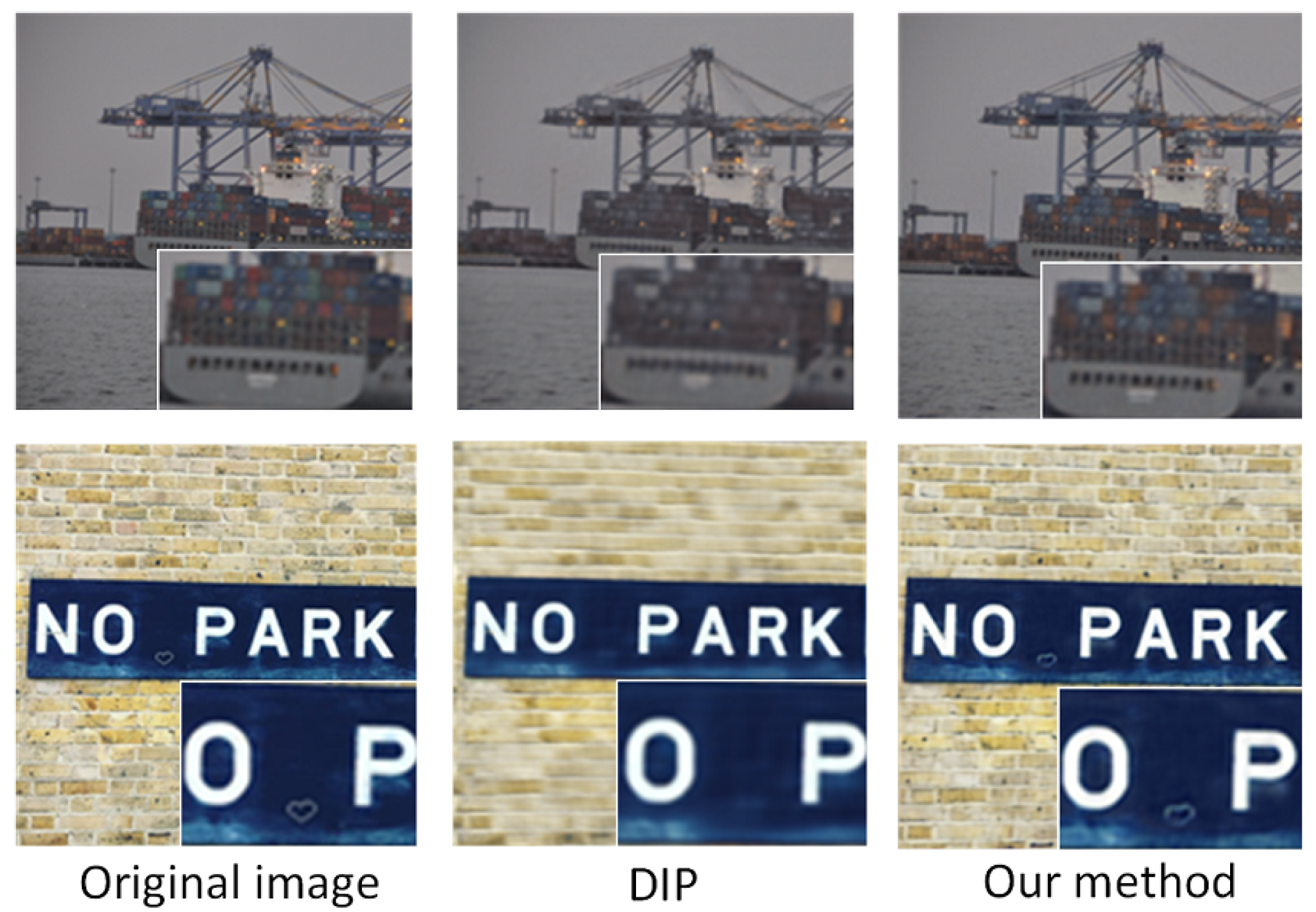
To prepare adversarial examples, we use Foolbox [38], a publicly available toolbox for adversarial attacks, to generate different adversarial examples, including FGSM, DeepFool, PGD, MI-FGSM, C&W. For each adversarial example, adversarial perturbations are considered under $L_{\infty }$ norm and the perturbation level $ϵ$ is set to 8.

4.2. DIP vs. t-DIPs

In this paper, we propose to use image restoration techniques to recover clean image from adversarial example. We design t-DIPs based on deep image prior network. The proposed method contains two DIP networks. The first network captures the main information of images and the second network recover original image based on the prior information provided by the first network. The experiments show that deep image prior alone is effective to defend against adversarial examples. However, the proposed method that uses multiple DIP networks needs fewer iterations and has better performance. The results are shown in Figure 6. For DIP, we choose U-Net which is same as the second DIP network in our method for comparison. Specifically, the number of iterations has a great influence on the performance of deep image prior networks. We set the number of iterations to 1500, and the classification accuracy is tested every one hundred intervals. For a full comparison, the number of iterations of the first DIP network is set to 100, 200 and 300.

It can be seen from Figure 6 that under all four attacks, our method outperforms DIP and requires fewer iterations. We also compare the impact of the first network iterations on the proposed method. It can be seen that in early iterations, classification accuracy increases with the increase of the first network iterations. That is because that the image with more iterations has more information. However, in late iterations, classification accuracy is almost not affected by the first network iterations. Besides, in strong attack BIM and MI-FGSM, classification accuracy first increases and then decreases with the increase of the number of iterations. That is because that adversarial perturbations are gradually learned with the iterations increasing. Thus, considering the balance of time and effect on different attacks, we set the first network iterations to 100, and the second network iterations to 1000.

Additionally, we also compared the subjective visual perception of the images generated by the single DIP and our method. Please refer to Figure 7 for details. The number of iterations is set to 1500. With a similar number of iterations, the images generated by our method is closer to the original images, which is better for the following model to classify.

4.3. Comparisons with Other Defensive Methods

To evaluate our proposed method, we compare our method with the current state-of-the-art defense based on image transformation, including HGD and ComDefend. We input the adversarial examples processed by different defense methods into the target model to calculate the accuracy. The higher accuracy represents the better defense effect. We apply different attacking methods including FGSM, DeepFool, BIM, MI-FGSM and C&W under the white-box settings to the following models: Inception-v3, ResNet152, ResNet50 and DenseNet161. The attacks have a maximum perturbation $ϵ=8$ for each pixel.

As shown in

Table 1. Performance comparison with state-of-the-art defenses on NIPS 2017 DEV images under white-box setting.

Defense	Clean	FGSM	DeepFool	BIM	MI-FGSM	C&W
Inception-v3
No Defense	86.4%	10.9%	1%	0%	0%	0%
HGD	81.7%	61.2%	80.8%	0.8%	0.4%	15.3%
ComDefend	63.3%	61.2%	63.4%	34%	40.2%	60.7%
Our method	67.2%	67.3%	68.1%	47.2%	53.6%	65.2%
ResNet152
No Defense	82.7%	3.4%	1.8%	0%	0%	0%
HGD	77.8%	50.5%	76.3%	3.4%	4%	37.2%
ComDefend	62%	51.9%	54.3%	26.4%	34.7%	50.8%
Our method	64.6%	60.7%	63.2%	39%	45.9%	60.8%
DenseNet161
No Defense	79.6%	1.3%	1.5%	0%	0%	0%
HGD	73.7%	41.4%	71.3%	2.6%	2.8%	28.8%
ComDefend	61%	50.8%	52.3%	23.5%	28.7%	50.1%
Our method	60.8%	56%	59.2%	24.6%	33.8%	52.4%
ResNet50
No Defense	76.7%	1.9%	1.4%	0%	0%	0%
HGD	72.5%	46%	70.3%	3.8%	4.2%	32.9%
ComDefend	55%	44.5%	46.3%	22.1%	28.2%	44.4%
Our method	59.2%	56%	55.3%	32.5%	40.6%	54.4%

Bold: represents the highest defense success rate.

, the proposed defense outperforms across four different models and various adversarial attacks. In particular, performance is improved a lot on defending strong attacks including BIM, MI-FGSM and C&W attack methods. Compared to HGD, the proposed method achieves higher accuracy on the FGSM, BIM, MI-FGSM and C&W attack methods. Specifically, performance is more balanced by using the proposed method on various adversarial attacks and original images. Although HGD performs well on original images and DeepFool attack, it performs extremely poorly on strong attacks. Compared to ComDefend, the proposed defense consistently improves the performance of defending various adversarial attacks. The accuracy of original images also increases. What’s more, unlike these existing defenses, which require training pre-processing module, the proposed method is training-free. It can be used directly as a plug-in module. In general, without training data and time, our method achieves much higher accuracy than the current state-of-the-art method on defense against most of adversarial attacks.

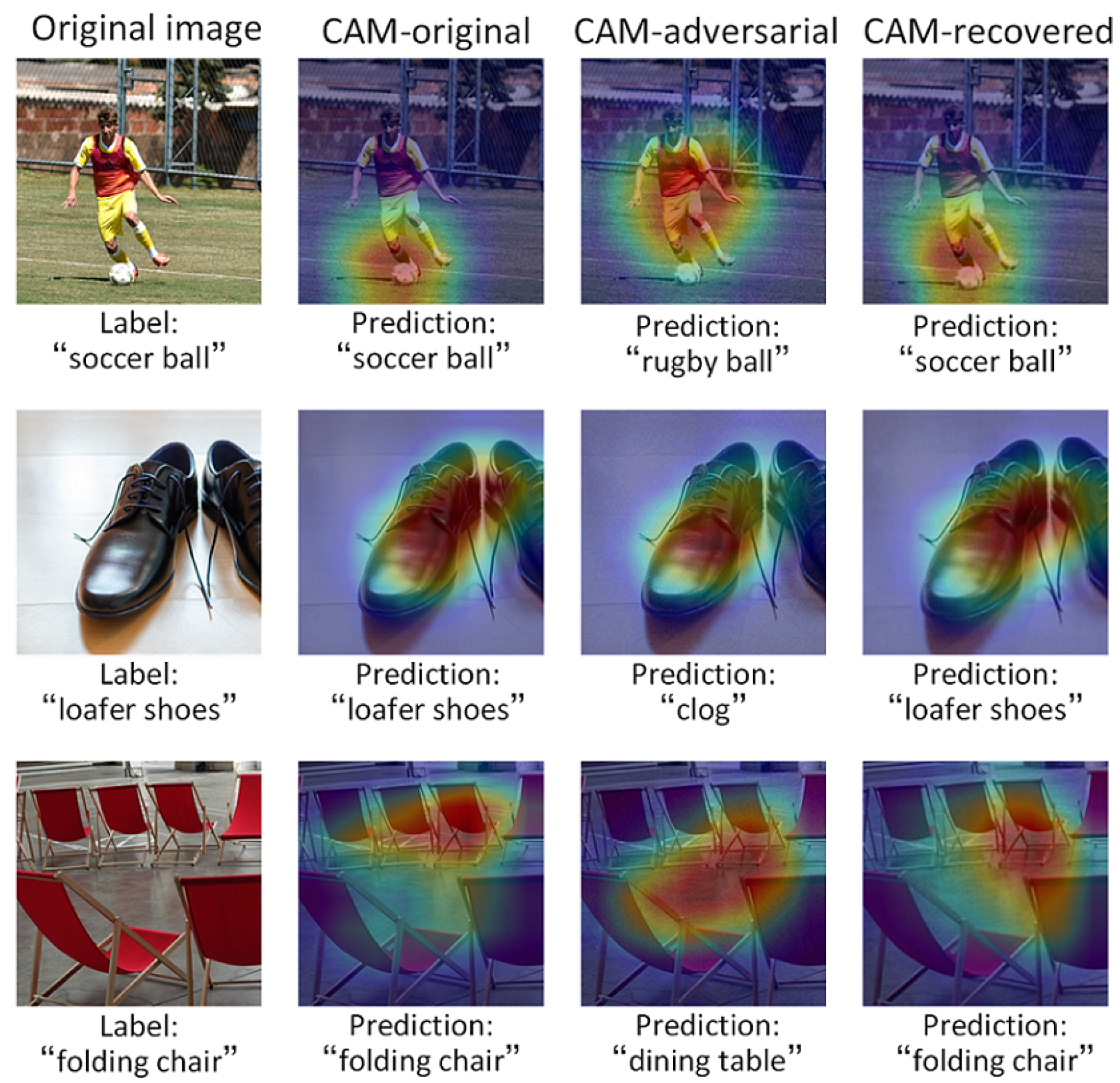
4.4. Analysis of the Proposed Method

To explore the nature of the proposed method we use localization techniques, termed Class Activation Maps (CAMs) [39]. CAM enables convolutional neural networks with global average pooling to localize the discriminative regions in the image. This method allows us to visualize the predicted class scores on a given image. In CAM, the red highlighted area means the area which network focus on. The features of this area have a greater weight on the network’s prediction. Figure 8 shows the CAMs for the top-1 prediction of Inception-v3 model for original, adversarial and recovered images. It can be seen that the network focus on the areas where soccer, shoes, and chair are located in original images. Thus, the network can predict correctly. However, for adversarial examples, adversarial perturbations make the network focus on the wrong regions, resulting in a wrong prediction. The CAMs of recovered images are closer to the CAMs of the original images. It is indicated that the proposed method is effective in keeping the original image content and suppressing adversarial perturbations.

5. Conclusions

The existence of adversarial examples brings a serious threat to the application of DNN in security-sensitive scenarios, such as autonomous vehicles. If the automatic driving system misclassifies the “stop” sign replaced with the adversarial example, it will be extremely dangerous. Therefore, it is necessary to explore robust defense methods. In this paper, we design tandem deep image prior networks, which recover the original images according to adversarial examples. The architecture of tandem network reduces the number of iterations required and achieving better performance. The proposed method is unsupervised, does not require training on adversarial examples. Thus, it is agnostic to the deployed model and attack method. Our work demonstrates that the proposed method performs better on FGSM, BIM, MI-FGSM, C&W attack methods, compared to the state-of-the-art defense method.

The limitations to our defense are that we only try U-Net type architecture in current experiments, and it still takes longer time than other defense methods. The quality of recovered images and the number of iterations needed are related to the architecture of network. In future work, we aim to design a more appropriate network to deal with adversarial examples. Besides, we hope to apply the proposed framework for more image restoration problems such as inpainting and super-resolution.

References

1. Lecun, Y.; Bengio, Y.; Hinton, G.E. Deep learning. Nature 2015, 521, 436–444. [Google Scholar] [CrossRef] [PubMed]
2. Krizhevsky, A.; Sutskever, I.; Hinton, G.E. Imagenet classification with deep convolutional neural networks. In Proceedings of the Advances in Neural Information Processing Systems, Lake Tahoe, NV, USA, 3–6 December 2012; pp. 1097–1105. [Google Scholar]
3. Hinton, G.E.; Deng, L.; Yu, D.; Dahl, G.E.; Mohamed, A.; Jaitly, N.; Senior, A.W.; Vanhoucke, V.; Nguyen, P.; Sainath, T.N.; et al. Deep Neural Networks for Acoustic Modeling in Speech Recognition: The Shared Views of Four Research Groups. IEEE Signal Process. Mag. 2012, 29, 82–97. [Google Scholar] [CrossRef]
4. Collobert, R.; Weston, J. A unified architecture for natural language processing: Deep neural networks with multitask learning. In Proceedings of the 25th International Conference on Machine Learning, Helsinki, Finland, 5–9 July 2008; pp. 160–167. [Google Scholar]
5. Szegedy, C.; Zaremba, W.; Sutskever, I.; Bruna, J.; Erhan, D.; Goodfellow, I.; Fergus, R. Intriguing properties of neural networks. arXiv 2013, arXiv:1312.6199. [Google Scholar]
6. Goodfellow, I.; Shlens, J.; Szegedy, C. Explaining and Harnessing Adversarial Examples. arXiv 2014, arXiv:1412.6572. [Google Scholar]
7. Kwon, H.; Kim, Y.; Yoon, H.; Choi, D. Random untargeted adversarial example on deep neural network. Symmetry 2018, 10, 738. [Google Scholar] [CrossRef] [Green Version]
8. Kurakin, A.; Goodfellow, I.; Bengio, S. Adversarial examples in the physical world. arXiv 2016, arXiv:1607.02533. [Google Scholar]
9. Evtimov, I.; Eykholt, K.; Fernandes, E.; Kohno, T.; Li, B.; Prakash, A.; Rahmati, A.; Song, D. Robust Physical- World Attacks on Deep Learning Models. Cryptogr. Secur. 2017, 2, 4. [Google Scholar]
10. Athalye, A.; Engstrom, L.; Ilyas, A.; Kwok, K. Synthesizing robust adversarial examples. In Proceedings of the International Conference on Machine Learning, Stockholm, Sweden, 10–15 July 2018; pp. 284–293. [Google Scholar]
11. Xu, X.; Zhao, H.; Jia, J. Dynamic Divide-and-Conquer Adversarial Training for Robust Semantic Segmentation. In Proceedings of the Computer Vision and Pattern Recognition, Seattle, WA, USA, 16–20 June 2020. [Google Scholar]
12. Du, X.; Yu, J.; Yi, Z.; Li, S.; Ma, J.; Tan, Y.; Wu, Q. A Hybrid Adversarial Attack for Different Application Scenarios. Appl. Sci. 2020, 10, 3559. [Google Scholar] [CrossRef]
13. Xie, C.; Wang, J.; Zhang, Z.; Ren, Z.; Yuille, A. Mitigating adversarial effects through randomization. arXiv 2017, arXiv:1711.01991. [Google Scholar]
14. Zhou, Y.; Kantarcioglu, M.; Xi, B. Efficacy of defending deep neural networks against adversarial attacks with randomization. In Proceedings of the Artificial Intelligence and Machine Learning for Multi-Domain Operations Applications II, Bellingham, WA, USA, 27 April–8 May 2020; Volume 11413, p. 114130Q. [Google Scholar]
15. Liao, F.; Liang, M.; Dong, Y.; Pang, T.; Hu, X.; Zhu, J. Defense against adversarial attacks using high-level representation guided denoiser. In Proceedings of the IEEE Conference on Computer Vision and Pattern Recognition, Salt Lake City, UT, USA, 18–23 June 2018; pp. 1778–1787. [Google Scholar]
16. Jia, X.; Wei, X.; Cao, X.; Foroosh, H. Comdefend: An efficient image compression model to defend adversarial examples. In Proceedings of the IEEE Conference on Computer Vision and Pattern Recognition, Long Beach, CA, USA, 15–20 June 2019; pp. 6084–6092. [Google Scholar]
17. Madry, A.; Makelov, A.; Schmidt, L.; Tsipras, D.; Vladu, A. Towards Deep Learning Models Resistant to Adversarial Attacks. arXiv 2017, arXiv:1706.06083. [Google Scholar]
18. Tramer, F.; Kurakin, A.; Papernot, N.; Goodfellow, I.; Boneh, D.; Mcdaniel, P. Ensemble Adversarial Training: Attacks and Defenses. arXiv 2017, arXiv:1705.07204. [Google Scholar]
19. Kannan, H.; Kurakin, A.; Goodfellow, I. Adversarial Logit Pairing. arXiv 2018, arXiv:1803.06373. [Google Scholar]
20. Grosse, K.; Manoharan, P.; Papernot, N.; Backes, M.; Mcdaniel, P. On the (Statistical) Detection of Adversarial Examples. arXiv 2017, arXiv:1702.06280. [Google Scholar]
21. Gong, Z.; Wang, W.; Ku, W. Adversarial and Clean Data Are Not Twins. arXiv 2017, arXiv:1704.04960. [Google Scholar]
22. Frosst, N.; Sabour, S.; Hinton, G.E. DARCCC: Detecting Adversaries by Reconstruction from Class Conditional Capsules. arXiv 2018, arXiv:1811.06969. [Google Scholar]
23. Ulyanov, D.; Vedaldi, A.; Lempitsky, V. Deep image prior. In Proceedings of the IEEE Conference on Computer Vision and Pattern Recognition, Salt Lake City, UT, USA, 18–22 June 2018; pp. 9446–9454. [Google Scholar]
24. Kurakin, A.; Goodfellow, I.; Bengio, S. Adversarial Machine Learning at Scale. In Proceedings of the Computer Vision and Pattern Recognition, Las Vegas, NV, USA, 27–30 June 2016. [Google Scholar]
25. Dong, Y.; Liao, F.; Pang, T.; Su, H.; Zhu, J.; Hu, X.; Li, J. Boosting adversarial attacks with momentum. In Proceedings of the IEEE Conference on Computer Vision and Pattern Recognition, Salt Lake City, UT, USA, 18–22 June 2018; pp. 9185–9193. [Google Scholar]
26. Carlini, N.; Wagner, D. Towards evaluating the robustness of neural networks. In Proceedings of the 2017 IEEE Symposium on Security and Privacy (sp), San Jose, CA, USA, 25 May 2017; pp. 39–57. [Google Scholar]
27. Fan, W.; Sun, G.; Deng, X. RGN-Defense: Erasing adversarial perturbations using deep residual generative network. J. Electron. Imaging 2019, 28, 013027. [Google Scholar] [CrossRef]
28. Entezari, N.; Papalexakis, E.E. TensorShield: Tensor-based Defense Against Adversarial Attacks on Images. arXiv 2020, arXiv:2002.10252. [Google Scholar]
29. Xie, C.; Wu, Y.; Der Maaten, L.V.; Yuille, A.L.; He, K. Feature Denoising for Improving Adversarial Robustness. In Proceedings of the Computer Vision and Pattern Recognition, Salt Lake City, UT, USA, 18–20 June 2018. [Google Scholar]
30. Jeddi, A.; Shafiee, M.J.; Karg, M.; Scharfenberger, C.; Wong, A. Learn2Perturb: An End-to-end Feature Perturbation Learning to Improve Adversarial Robustness. In Proceedings of the Computer Vision and Pattern Recognition, Seattle, WA, USA, 16–20 June 2020. [Google Scholar]
31. Freitas, S.; Chen, S.; Wang, Z.; Chau, D.H. UnMask: Adversarial Detection and Defense Through Robust Feature Alignment. In Proceedings of the Computer Vision and Pattern Recognition, Seattle, WA, USA, 16–20 June 2020. [Google Scholar]
32. Szegedy, C.; Vanhoucke, V.; Ioffe, S.; Shlens, J.; Wojna, Z. Rethinking the inception architecture for computer vision. In Proceedings of the Conference on Computer Vision and Pattern Recognition, Las Vegas, NV, USA, 27–30 June 2016; pp. 2818–2826. [Google Scholar]
33. Ronneberger, O.; Fischer, P.; Brox, T. U-net: Convolutional networks for biomedical image segmentation. In Proceedings of the International Conference on Medical Image Computing and Computer-Assisted Intervention, Munich, Germany, 5–9 October 2015; pp. 234–241. [Google Scholar]
34. He, K.; Zhang, X.; Ren, S.; Sun, J. Deep residual learning for image recognition. In Proceedings of the IEEE Conference on Computer Vision and Pattern Recognition, Las Vegas, NV, USA, 27–30 June 2016; pp. 770–778. [Google Scholar]
35. Huang, G.; Liu, Z.; Van Der Maaten, L.; Weinberger, K.Q. Densely connected convolutional networks. In Proceedings of the IEEE Conference on Computer Vision and Pattern Recognition, Honolulu, HI, USA, 21–26 July 2017; pp. 4700–4708. [Google Scholar]
36. Kurakin, A.; Goodfellow, I.; Bengio, S.; Dong, Y.; Liao, F.; Liang, M.; Pang, T.; Zhu, J.; Hu, X.; Xie, C.; et al. Adversarial Attacks and Defences Competition. In Proceedings of the Computer Vision and Pattern Recognition, Salt Lake City, UT, USA, 18–23 June 2018; pp. 195–231. [Google Scholar]
37. Kingma, D.P.; Ba, J. Adam: A method for stochastic optimization. arXiv 2014, arXiv:1412.6980. [Google Scholar]
38. Rauber, J.; Brendel, W.; Bethge, M. Foolbox v0.8.0: A Python toolbox to benchmark the robustness of machine learning models. arXiv 2017, arXiv:1707.04131. [Google Scholar]
39. Zhou, B.; Khosla, A.; Lapedriza, A.; Oliva, A.; Torralba, A. Learning deep features for discriminative localization. In Proceedings of the IEEE Conference on Computer Vision and Pattern Recognition, Las Vegas, NV, USA, 27–30 June 2016; pp. 2921–2929. [Google Scholar]
Figure 1. DNN provides the wrong prediction with high confidence by adding imperceptible perturbations to the original image.
Electronics 09 01957 g001
Figure 2. The main idea of t-DIPs. The first network DIP 1 captures the main information of the image. The second network DIP 2 generates the corresponding clean image based on the output of network DIP 1 . The two DIP networks set the loss function as minimizing the difference of recovery image and adversarial example.
Electronics 09 01957 g002
Figure 3. The ability of deep image prior to recover original image from adversarial example. The accuracy of Inception v-3 with no defense is 0%.
Electronics 09 01957 g003
Figure 4. The structure of the network DIP 1 .
Electronics 09 01957 g004
Figure 5. The structure of the network DIP 2 .
Electronics 09 01957 g005
Figure 6. The classification accuracy of Inception-v3 on adversarial images generated by four attacks. The blue line represents the accuracy of Inception-v3 with DIP for defense.
Electronics 09 01957 g006
Figure 7. Comparison of images generated by our method with a single DIP network. With a similar number of iterations, our method can reconstruct images with more details.
Electronics 09 01957 g007
Figure 8. Class activation maps for original, adversarial and recovered images.
Electronics 09 01957 g008