Vehicular Navigation Based on the Fusion of 3D-RISS and Machine Learning Enhanced Visual Data in Challenging Environments

Abstract

Based on the 3D Reduced Inertial Sensor System (3D-RISS) and the Machine Learning Enhanced Visual Data (MLEVD), an integrated vehicle navigation system is proposed in this paper. In demanding conditions such as outdoor satellite signal interference and indoor navigation, this work incorporates vehicle smooth navigation. Firstly, a landmark is set up and both of its size and position are accurately measured. Secondly, the image with the landmark information is captured quickly by using the machine learning. Thirdly, the template matching method and the Extended Kalman Filter (EKF) are then used to correct the errors of the Inertial Navigation System (INS), which employs the 3D-RISS to reduce the overall cost and ensuring the vehicular positioning accuracy simultaneously. Finally, both outdoor and indoor experiments are conducted to verify the performance of the 3D-RISS/MLEVD integrated navigation technology. Results reveal that the proposed method can effectively reduce the accumulated error of the INS with time while maintaining the positioning error within a few meters.

1. Introduction

Navigation technology is becoming increasingly important in different aspects of daily life. Positioning and navigation technologies for outdoor environments has dramatically developed, a typical example is the Global Positioning System (GPS) [1,2]. In densely populated commercial or public places, there is a growing demand for the location navigation, environment awareness and real-time monitoring of people. Moreover, the indoor positioning technology should provide sufficiently accurate location services to the users.

Integration of the Inertial Navigation System (INS) and the GPS is widely utilized to accurately determine the position and the attitude of the moving objects. The GPS has the advantages of providing absolute positioning with long-time stability and mid-level precision. The INS, on the other hand, has a good short-term accuracy and does not rely on any external sources for determining the position, velocity and attitude. However, the INS is prone to severe drift errors, especially when dealing with the commercial-grade systems [3]. Additionally, the GPS could suffer from signal blockage, interference and multipath. This could result in extended periods of GPS signal outage, which occurs in urban canyons, forests and indoors. What’s worse, the positioning error of GPS would sharply increase especially in indoors. Therefore, a vision system to aid the INS is proposed to enhance the overall solution in such situations and keeping the cost to a minimum level [4,5]. The visual positioning is based on the image sequence to achieve the positioning. The feature points are extracted and matched to the acquired image sequence, and the matched feature points are then utilized to solve the transformation relationship of different frame images, and so the motion parameters are estimated. It is also possible to set up the landmarks [6] and measure their information in advance, and then obtain the vehicular position through the vehicle matching landmarks to achieve the purpose of precisely navigation. In the literature, some works that focus on the INS [7,8,9] and vision had been done. Martinelli A. [7] proposed a monocular vision and inertial navigation fusion algorithm to determine the motion parameters of a vehicle moving in 3D unknown environment. The measurement data of the monocular and inertial sensors in a short time interval were fused and estimated. The algorithm outputs the vehicular velocity and attitude, as well as the absolute scale and the deviation that affect the inertial measurement. To reduce the positioning error of the aircraft and loosely couple the monocular vision and inertial sensors positioning data, an integrated Extended Kalman Filter (EKF) method was presented in [8]. The positioning data of the inertial navigation system is used to compensation the result of visual location. In [9], aiming at the pose estimation problem of small unmanned aerial vehicles with GPS unavailability, a monocular camera with low-cost Inertial Measurement Unit (IMU) installed on a drone was presented, and the fusion is completed by EKF for navigation.

Recently, Deep Artificial Neural Networks (DANNs) have promoted significant breakthroughs in pattern recognition and machine learning [10]. Furthermore, Convolutional Neural Networks (CNNs) have been successfully applied to a variety of recognition and classification tasks [11,12,13,14]. Compared to the standard feed forward neural networks with similarly sized layers, CNNs have much fewer connections and parameters. Hence, they are much easier to be trained [15]. Deep learning methods allow machines to be fed with raw data and then facilitate automatic discovery of the representations required for detection and classification; in particular, they enable a model to work in an end-to-end manner [16]. Nowadays, there are some works serve for robot navigation based on deep learning [17,18,19]. They apply the neural network process raw sensors’ data to complete the navigation and obstacle avoidance tasks. Current object recognition methods are strongly dependent on deep learning and large datasets and there are many techniques for preventing overfitting during model training, such as early stopping and dropping out. Therefore, the deep learning is indispensable in image classification.

Tai et al. [18] proposed an indoor obstacle avoidance solution based on deep network and sensors data. Their robot decisions show a high similarity with human decisions. Zhu et al. [19] presented an indoor navigation method based on visual input. Their robot can successfully search for the given target and learn the relationships between actions and environment. They applied deep learning and reinforcement learning technique avoiding the feature matching process during navigating. Hussein et al. [20] demonstrated the reinforcement learning based navigation method employ DCNNs and learn directly from the raw visual input. The model they trained can successfully learn the navigation policy from visual input while learning from experience. Through the combination with vision system, the navigation robot could enhance the positioning accuracy while carrying our target recognition, target tracking and target detection tasks.

In this study, a new integrated positioning system including inertial navigation and Machine Learning Enhanced Visual Data (MLEVD) is proposed. Specifically, the 3D Reduced Inertial Sensor System (3D-RISS) based inertial navigation could reduce the costs and maintain a high accuracy rate. The monocular vision oversees the supplement of the positioning requirements of the vehicle. Moreover, in the application of CNNs, a particular class of neural networks that shows a promising performance in object recognition, is utilized to enhance the speed of processor. During the first phase of our approach, the model extracts the landmarks from the visual scene that is input using the camera. Then, the CNN outputs the prediction of the current road or building information by a multi-label classifier. Furthermore, the position of the vehicle can be obtained by template matching with landmarks that are pre-setup and the corresponding size and position are also computed. After that, the EKF method is utilized for the fusion of the location signals from both the neural network model and the inertial sensors to calculate the current position of the vehicle. Finally, the feasibility of the algorithm is verified through the outdoor and indoor experiments. Results show that the proposed approach could effectively reduce the accumulated error of the INS with time while maintaining the positioning error within a few meters for outdoor experiments and less than 1 m for indoor experiments.

2. Formulation

2.1. Convolution Neural Network

The CNNs are similar to the ordinary neural networks. The convolution is performed at the convolutional layers to extract features from local neighborhood on feature maps in the previous layer. It is the core block of a convolutional network. Among the layers of neural network, we use the Rectified Linear Units (ReLUs) [21] as the activation function to train the model with gradient descent method. One advantage of the ReLUs is that they don’t require the normalization of input to avoid saturating. CNN is a hierarchical network for feature extraction with back-propagating the gradients of errors. Convolution, non-linear activation and pooling are three main operations of the featured hierarchy.

The convolution operation takes the weighted sum of pixel values in a receptive field. Equation (1) shows its mathematical expression:

$$y_{ijk}={(W_i*x)}_{ik}+b_i$$

(1)

where $y_{ijk}$ is the pixel value at coordinate $(j,k)$ of $i$—the output feature map, $W$ is the convolution kernel, $x$ is the input and $b$ is related bias vector. The non-linear activation, ReLUs $f(x)=\max (0,x)$, is applied after convolution. ReLUs has the piece-wise linear property.

The pooling layer summarizes the outputs of adjacent neurons in the same kernel map. During our training, we applied the overlapping pooling which produces an output of equivalent dimensions as the input. It takes the maximum or average value in an image batch to enhance the robustness of the network. The stride parameter exists in the pooling layer and convolution layer. It is several moving steps over pixels of convolution.

The last layer is an output layer that is chosen based on the task. For binary classification tasks, there are only two neurons needed to compose the output layer. On the other hand, for a multi-label classification tasks, the neurons of output layer are designed based on the actual number of categories. Normally, the output layer is a standard fully connected layer.

To reduce the test errors, there are some works that combine the predictions of many models [22,23]. However, for an object recognition task, it is expense to train many models and combine their results. Therefore, we adopt the dropout technique. The dropout is a technique that randomly disconnects the neurons from the current layer to the next layer. This random disconnecting helps the network to reduce the overfitting because no single neuron in the layer will be responsible for predicting a certain class, object, edge or corner. In this research work, 25% dropout rate is adopted to avoid the overfitting.

2.2. Visual System

2.2.1. Camera Calibration and Correction of Distorted Image

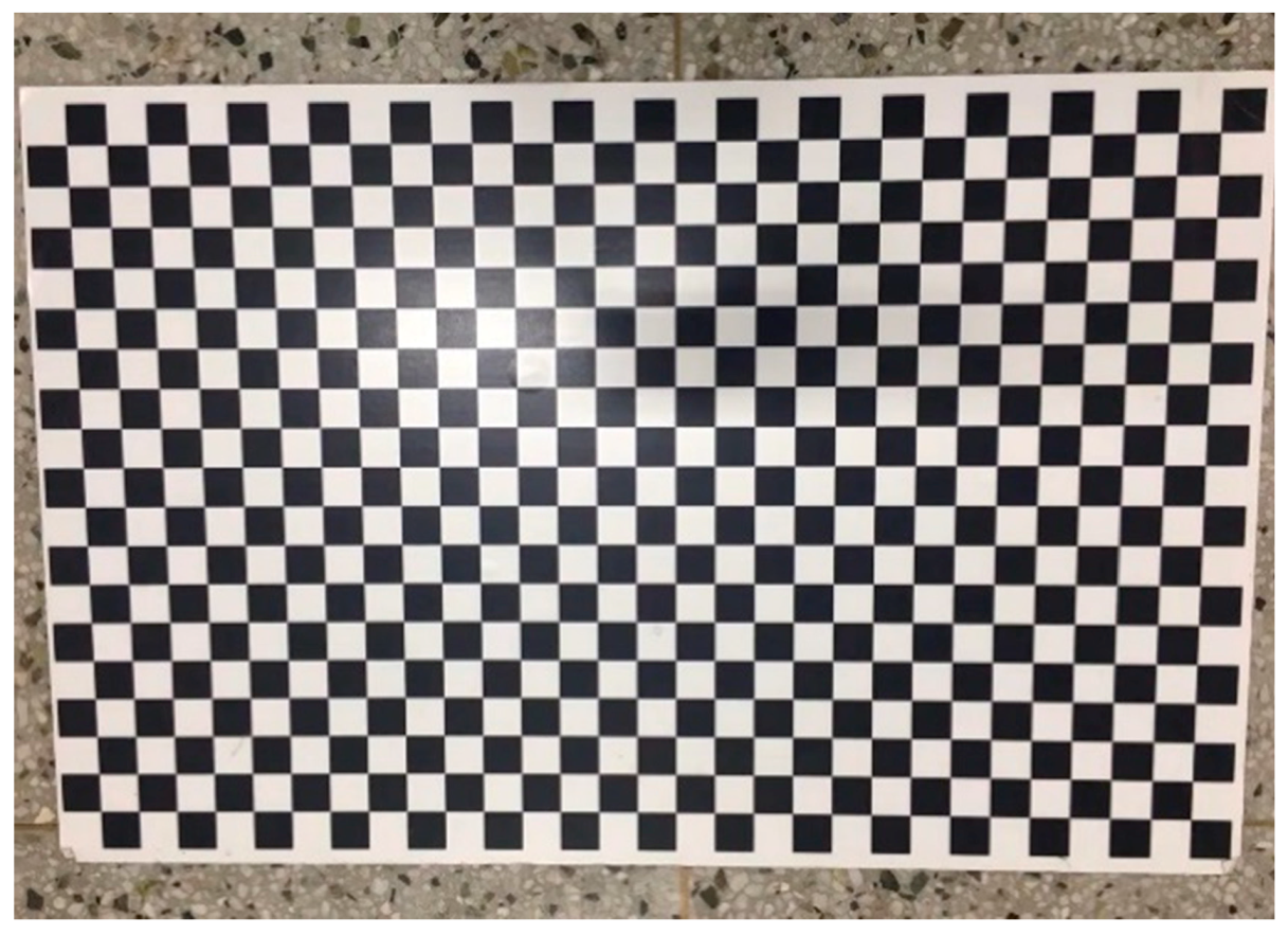
Camera calibration is a procedure for estimating the intrinsic parameters K and radial distortion parameters P of a given camera. It is usually finished by taking several images of a checkerboard from different angles and different distances. From these images, and given the size of a checkerboard square, the intrinsic parameters can be estimated. Using these parameters can achieve the purpose of correcting the distortion of the picture. The method is described with details in the literatures [24,25,26].

The checkerboard of camera calibration is shown in Figure 1. The side length of each square is 4 cm. After calibration K and P are solved as:

$$K=\left[\begin{array}{ccc}3424.07& 0& 0\\ 0& 3434.69& 0\\ 1693.12& 1203.11& 1\end{array}\right],P=(-0.448,0.2235,0).$$

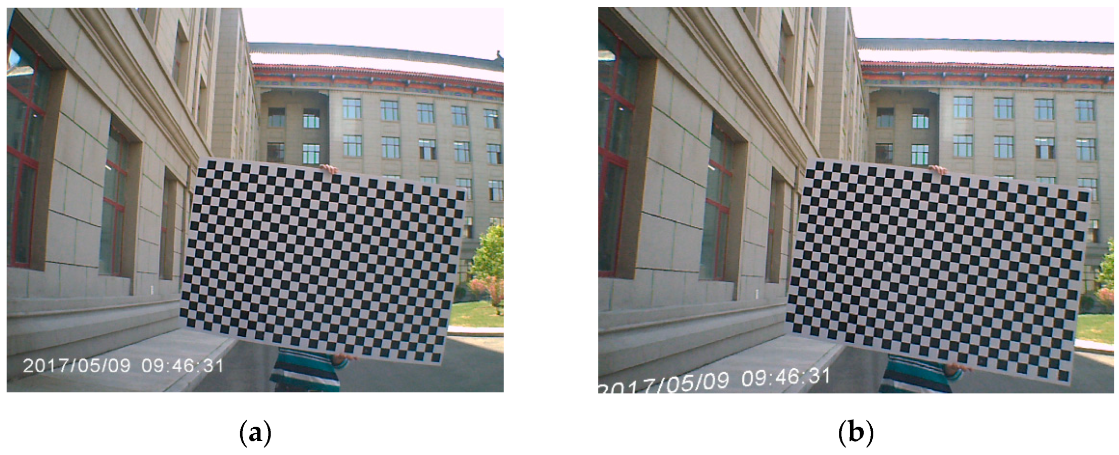
The distortion can be corrected by tuning the parameters of K and P. Figure 2 shows the comparison between the original image and the correcting distortion image. It can be demonstrated that the straight lines in the picture become no longer curved after correcting distortion especially at the edges of the image.

2.2.2. Template Matching

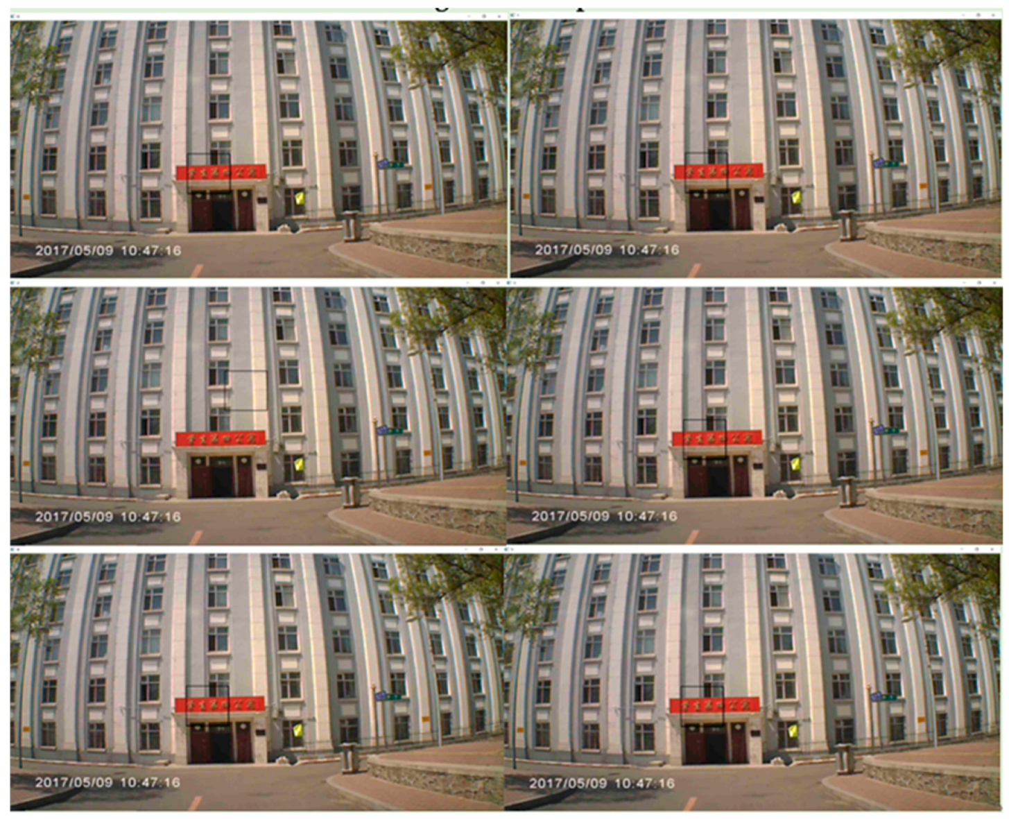
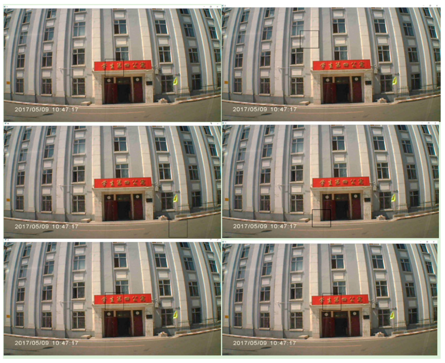
Images are extracted from the video stream captured by a camera on-board the vehicle. For each image, a smaller scanning block with several pixels (width and height), are swept from the top left corner to the bottom right corner. The similarity between the part of the image within the scanning block and a predetermined landmark from the pre-captured image is computed. When a good match is searched, the pixel location of the landmark in the extracted image is recorded. This pixel location is then compared with the pixel location of the landmark in the original pre-captured image. Given that the two-pixel locations are within a distance threshold, we determine our position as the original pre-captured known image position. There are six methods for the determination: matching by difference of squares, normalizing the difference of squares, determining the correlation, normalizing the correlation, calculating the correlation coefficient and normalizing the correlation coefficient [27].

Each matching method could provide a decision area of the same size as the template and determine the position of the area. Next, we determine whether the results of the six methods are consistent.

Once the trajectory commences, the top left corner ($x_l$, $y_l$) of the best cross correlation match R($x_l$, $y_l$) is determined for each method. The best match for the landmark position from each method is (${\mathrm{x}}_m$, ${\mathrm{y}}_m$), where m = 1, 2, 3, 4, 5, 6.

Next, the distance between the landmark locations in pixels as determined from each method is computed ($d_{ij}$; i = 1, 2, 3, 4, 5, 6; j = 1, 2, 3, 4, 5, 6; i ≠ j):

$$d_{ij}=\sqrt{{\left(x_i-x_j\right)}^2+{\left(y_i-y_j\right)}^2}$$

(2)

If $d_{ij}$ ≤ α, then the results of method i and method j are taken to be the same. Let S be the number of elements in $d_{ij}$ that satisfy the condition $d_{ij}$ ≤ α. For a small α, if S is large, we can conclude that the matching algorithm is precise. If S = 15, the results of all methods are the same. Within the extracted image sequences captured by the vehicle camera, the image with the largest S is taken to be the correctly matched image. However, if S is too small, we conclude that there is no match.

2.2.3. Landmark Chosen

First, the characteristics of the driving recorder are measured. Because the linearity of the image size and distance recorded by the driving recorder is low, the proportional relationship between the distance from the camera to the landmark and the size of the landmark is a fixed value in one image.

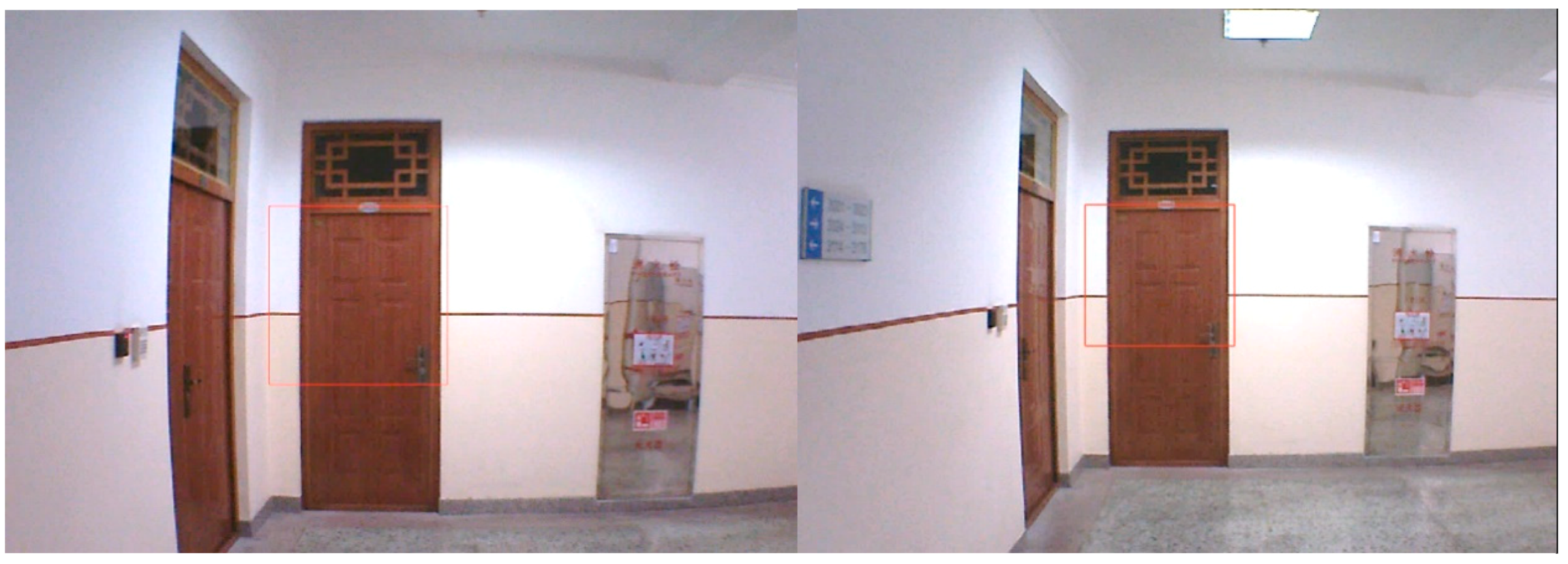
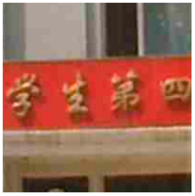
The landmark is chosen as in Figure 3. The image size is 1920 × 1080. The coordinates of the upper left corner are (0, 0) while those of the lower right corner are (1920, 1080). The red box in the image is the set landmark. The real size is 1.2 m × 1.2 m. The size of the landmark in the image is 432 × 432. The distance between the landmark and the camera is 6 m. When the distance is 7 m, the size of the landmark in the image is 379 × 379 and so on. The proportional relationship is shown in

Table 1. Proportional relationship between distance and landmark size.

Distance	6	7	8	9	10	11	12	…
Proportional	360	315.8	275	230.2	201.5	179	157.5	…

. Through this ratio, the size of pixels on the picture can be obtained for the landmarks of different sizes at different distances. Both the coordinate location and the size of every landmark are previously measured by GPS receiver and ruler respectively.

The landmarks are usually limited to the middle of the image, and they are generally set at the end of the straight road, it is considered that the signpost position is directly in front of the carrier and the experimental error is within an acceptable range. If the area is out of a fixed region of the picture, this matching is judged as invalid. If the area becomes smaller, the higher positioning accuracy would reach and the matched landmarks are less and less. For the same landmark, at least one template with a size can be successfully matched to obtain the position information. The coordinate of the landmark is ($lon{g}_l,la{t}_l$), the azimuth of the landmark is $\alpha$, and the distance between the landmark and the carrier is d. Therefore, the coordinate of the carrier, ($lon{g}_v$, $la{t}_v$), is given by

$$la{t}_v=arcsin(sin(la{t}_l)*cos(d/R)+cos(la{t}_l)*sin(d/R)*cos(a)),$$

(3)

$$lon{g}_v=lon{g}_l+arctan\frac{cos(d/R)-sin(la{t}_l)*sin(la{t}_v)}{sin(a)*sin(d/R)*cos(la{t}_l)},$$

(4)

where R is the radius of the Earth.

For landmarks that are not easy to be computed directly, their locations can be calculated by other point locations that is easy-to-computed using Equations (3) and (4), such as the landmarks in indoor environment.

2.3. 3D-RISS Mechanization

The IMU mechanization is performed using a 3D-RISS, which employs an odometer, a uniaxial gyroscope and a dual-axial accelerometer. It has been shown [28,29,30] that the 3D-RISS algorithm outperforms the conventional method of complete mechanization that uses tri-axial gyroscopes and accelerometers. The dead-reckoning position estimation from the 3D-RISS mechanization is then integrated with the vision data using an EKF [31,32,33]. The detailed results of the integration are presented in the next section.

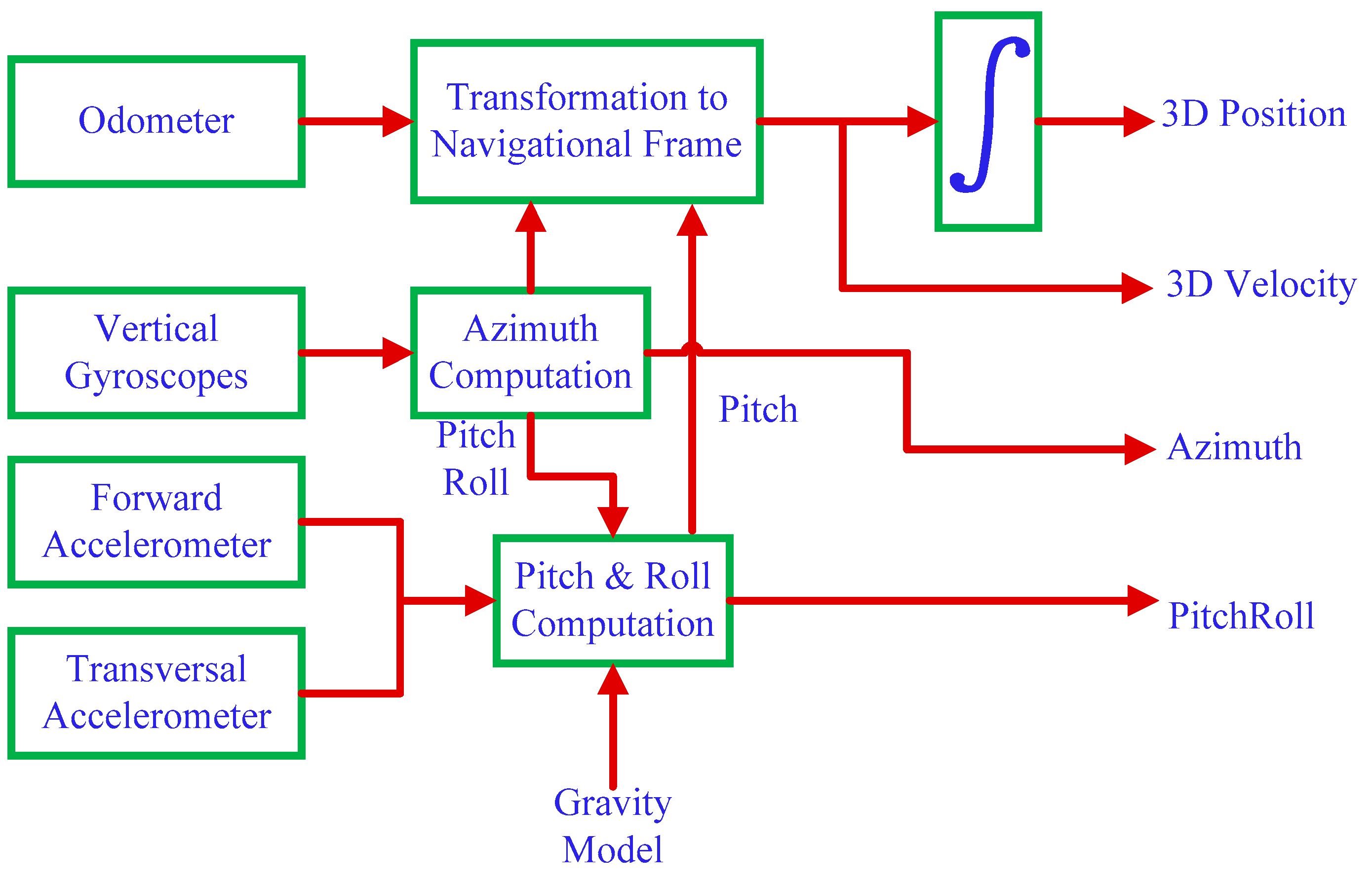
During the 3D-RISS mechanization process, the pitch angle of the vehicle is calculated using the forward accelerometer output information. The pitch angle p is calculated as

$$p={\sin }^{-1}(\frac{f_y-a_{od}}{g}).$$

(5)

where $f_y$ is the forward accelerometer measurement, a_od is the odometer rate of change of velocity and g is the acceleration due to gravity.

The schematic diagram of 3D-RISS mechanization is shown in Figure 4.

The roll angle of the moving vehicle r is calculated using the transversal accelerometer information $f_x$, the azimuth gyroscope measurement ${\omega }_z$ and the odometer velocity information $v_{od}$.

$$r=-{\sin }^{-1}\left(\frac{f_x+v_{od}{\omega }_z}{g\cos p}\right),$$

(6)

The azimuth angle $\dot{A}$ is given by

$$\dot{A}=-\left({\omega }_z-{\omega }^{ie}\sin \phi -\frac{v_e\tan \phi }{R_N+h}\right),$$

(7)

where ω^ie is the Earth rotation rate, $v_e$ is east velocity, φ is the latitude, h is the altitude of the vehicle and $R_N$ is the normal radius of curvature of the Earth’s ellipsoid.

Then, the local-level frame velocity is given by

$$v=\left[\begin{array}{c}{v}_e\\ v_n\\ v_u\end{array}\right]=\left[\begin{array}{c}{v}_{od}\sin A\cos p\\ v_{od}\cos A\cos p\\ v_{od}\sin p\end{array}\right],$$

(8)

where $v_e$, $v_n$, and $v_u$ denote the East, North and Upward velocities respectively, which are transformed from the vehicle’s speed along the forward direction v.

The 3D position is then obtained by

$$\begin{array}{c}\dot{h}=v_u,\\ \dot{\phi }=\frac{v_n}{R+h},\\ \dot{\lambda }=\frac{v_e}{(R+h)\cos \phi },\end{array}$$

(9)

where, $\dot{h}$, $\dot{\phi }$, and $\dot{\lambda }$ are the Altitude, Latitude and Longitude calculated by 3D-RISS, respectively. R is the meridian radius of curvature of the Earth’s ellipsoid.

2.4. Kalman Filter Design of 3D-RISS/MLEVD Integration

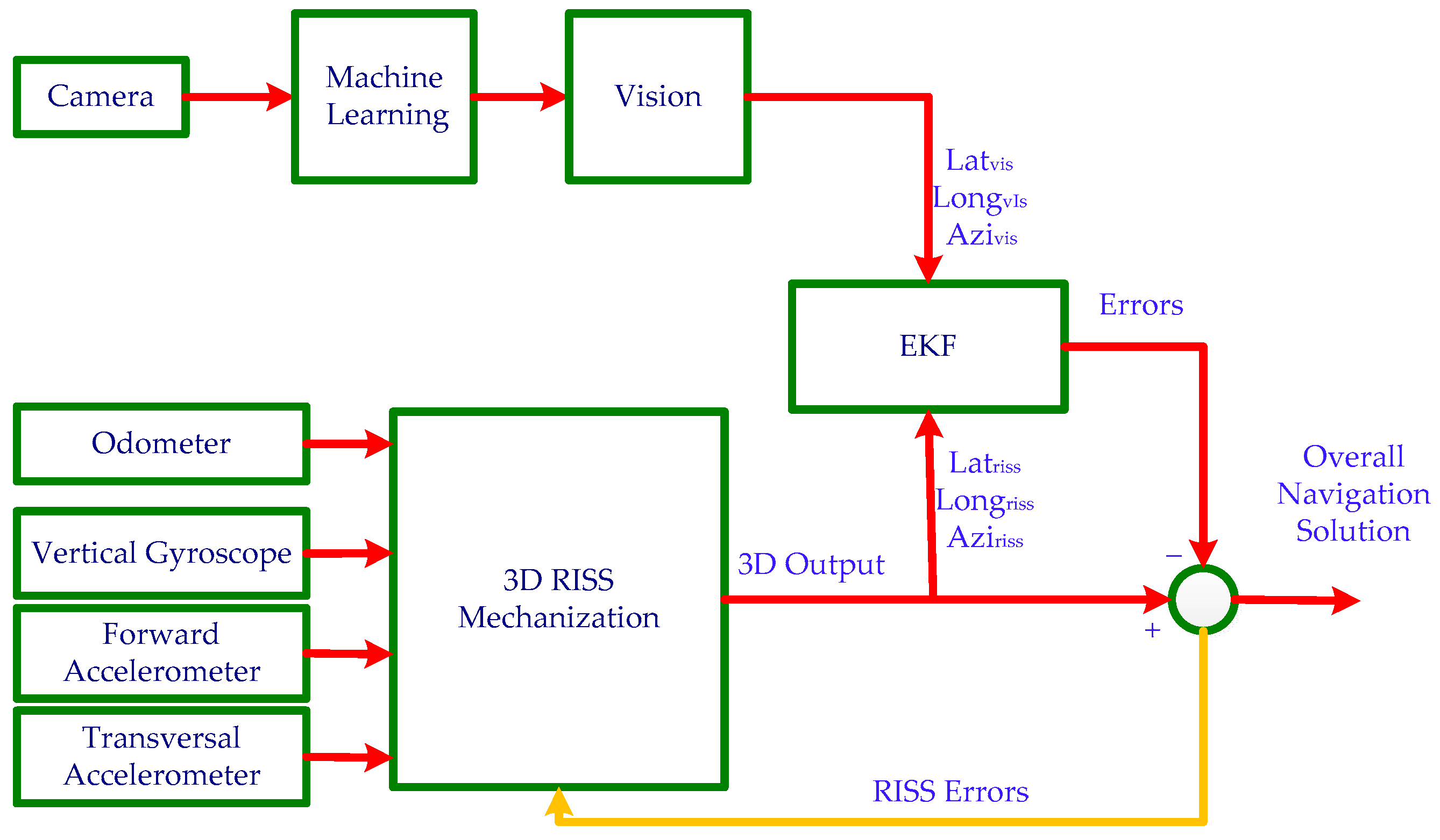
The block diagram of the 3D-RISS/MLEVD integrated navigation system is shown in Figure 5.

Through template matching, the camera can acquire the absolute Latitude, Longitude and azimuth angle of the robot when it passes the landmarks. The 3D-RISS algorithm calculates the robot position, velocity and orientation based on the IMU and odometer data. A Kalman filter integrates this information with the position and azimuth update from the camera.

The error state vector of the Kalman filter is defined as

$$\delta x=\left[\delta \phi ,\delta \lambda ,\delta h,\delta v^e,\delta v^n,\delta v^u,\delta A,\delta b_z,\delta a_{od}\right],$$

(10)

where $\delta \phi$ is the Latitude error, $\delta \lambda$ is the Longitude error, $\delta h$ is the Altitude error, $\delta v^e$ is the East velocity error, $\delta v^n$ is the North velocity error, $\delta v^u$ is the Upward velocity error, $\delta A$ is the azimuth error, $\delta a_{od}$ is the error in acceleration derived from odometer measurements and $\delta b_z$ is the error due to the gyroscope bias.

The motion Equations (8) and (9) are linearized by Taylor’s series expansion and only the first-order terms are retained [34,35]. The state transition matrix F is formulated below. F_ab identifies each non-zero element in matrix F, where the subscript a denotes the row and b denotes the column of the matrix.

$$\delta \dot{\phi }=\underset{F_{15}}{\underbrace{\frac{\delta v_n}{\left(R+h\right)}}},$$

(11)

$$\delta \dot{\lambda }=\underset{F_{24}}{\underbrace{\frac{1}{\left(R+h\right)\cos \phi }}}\delta v_e+\frac{v_e\tan \phi }{\underset{F_{21}}{\underbrace{\left(R+h\right)\cos \phi }}}\delta \phi ,$$

(12)

$$\dot{h}=\underset{F_{36}}{\delta v_u},$$

(13)

$$\begin{array}{l}\delta {\dot{v}}_e=\underset{F_{48}}{\underbrace{\sin A\cos p}}\delta a_0+\underset{F_{47}}{\underbrace{a_0\cos A\cos p}}\delta A-\underset{F_{45}}{\underbrace{\left({\omega }_z-b_z-{\omega }^e\sin \phi -\frac{v_e\tan \phi }{R+h}\right)}}\delta v_n+\underset{F_{49}}{v_n}\delta b_z\\ +\underset{F_{41}}{\underbrace{v_n\left({\omega }^e\cos \phi +\frac{v_e{\sec }^2\phi }{R+h}\right)}}\delta \phi +\frac{v_n\tan \phi }{\underset{F_{44}}{\underbrace{R+h}}}\delta v_e\end{array}$$

(14)

$$\begin{array}{l}\delta {\dot{v}}_n=\underset{F_{58}}{\underbrace{\cos A\cos p}}\delta a_0+\underset{F_{57}}{\underbrace{a_0\sin A\cos p}}\delta A+\underset{F_{54}}{\underbrace{\left({\omega }_z-b_z-{\omega }^e\sin \phi -\frac{2v_e\tan \phi }{R+h}\right)}}\delta v_e\\ -\underset{F_{59}}{v_e}\delta b_z-\underset{F_{51}}{\underbrace{v_e\left({\omega }^e\cos \phi +\frac{v_e{\sec }^2\phi }{R+h}\right)}}\delta \phi \end{array}$$

(15)

$$\delta {\dot{v}}_u=\underset{F_{68}}{\sin p}\delta a_0,$$

(16)

$$\delta \dot{A}=\underset{F_{79}}{\delta b_z}+\underset{F_{71}}{\underbrace{\left({\omega }^e\cos \phi +\frac{v_e{\sec }^2\phi }{R+h}\right)}}\delta \phi +\frac{\tan \phi }{\underset{F_{74}}{\underbrace{R+h}}}\delta v_e,$$

(17)

The drift error of the gyroscope and the error in the acceleration, which occurs because of the odometer, are modeled by first-order Gauss–Markov processes as given below [36]:

$$\delta {\dot{a}}_0=\underset{F_{88}}{-{\beta }_0}\delta a_0+\sqrt{2{\beta }_0{\sigma }_0^2}w\left(t\right),$$

(18)

$$\delta {\dot{b}}_z=\underset{F_{99}}{-{\beta }_z}\delta b_z+\sqrt{2{\beta }_z{\sigma }_z^2}w\left(t\right),$$

(19)

where β and σ are the reciprocal of the correlation time and the standard deviation of the respective errors.

The overall system dynamic matrix F is given by

$$F=\left[\begin{array}{ccccccccc}0& 0& 0& 0& F_{15}& 0& 0& 0& 0\\ F_{21}& 0& 0& F_{24}& 0& 0& 0& 0& 0\\ 0& 0& 0& 0& 0& F_{36}& 0& 0& 0\\ F_{41}& 0& 0& F_{44}& F_{45}& 0& F_{47}& F_{48}& F_{49}\\ F_{51}& 0& 0& F_{54}& 0& 0& F_{57}& F_{58}& F_{59}\\ 0& 0& 0& 0& 0& 0& 0& F_{68}& 0\\ F_{71}& 0& 0& F_{74}& 0& 0& 0& 0& F_{79}\\ 0& 0& 0& 0& 0& 0& 0& F_{88}& 0\\ 0& 0& 0& 0& 0& 0& 0& 0& F_{99}\end{array}\right],$$

(20)

The measurement model that relates the 3D-RISS system estimate to the vision-based solution is given by

$$z=H\delta x,$$

(21)

where H that relates the system state vector to the observations, is given by

$$H=\left[\begin{array}{ccccccccc}1& 0& 0& 0& 0& 0& 0& 0& 0\\ 0& 1& 0& 0& 0& 0& 0& 0& 0\\ 0& 0& 0& 0& 0& 0& 1& 0& 0\end{array}\right]$$

(22)

and Z can be written as

$$z=\left[\begin{array}{c}La{t}_{vis}-La{t}_{riss}\\ Lon{g}_{vis}-Lon{g}_{riss}\\ Az{i}_{vis}-Az{i}_{riss}\end{array}\right],$$

(23)

where Lat_vis, Long_vis, and Azi_vis are the Latitude, Longitude and azimuth determined by the vision, while Lat_riss, Long_riss, and Azi_riss are the Latitude, Longitude and azimuth estimated by the 3D-RISS.

After the complete system model and measurement model are established, the EKF error state vector and covariance matrix are utilized to implement the prediction step. When a landmark is detected, the Kalman gain is calculated and the error state vector is updated accordingly.

3. Verification Experiments and Results Analysis

Both outdoor experiment and indoor experiment are conducted here to verify the performance of the 3D-RISS/MLEVD integrated navigation technology in different challenging environments.

3.1. Outdoor Experiment

The outdoor experiment involves the integration of the inertial navigation with MLEVD. The experimental equipment used are the FFG-16 INS [37], a set of driving recorders and high-precision RTK GPS, which are installed and shown in Figure 6. Because of the arithmetic of 3D-RISS, only 1 gyroscope and 2 accelerometers of FFG-16 were used, and their parameters are summarized in

Table 2. Performance of the gyroscope and accelerometer in FFG-16.

	Performance	FFG-16
Gyroscope	Bias stability (°/h)	≤0.01
	Nonlinear degree of scale factor (ppm)	≤3
	Resolution (°/s)	0.0005
	Dynamic range (°/s)	≤600
	Random walk coefficient (°/h1/2)	0.003
Accelerometer	Input range (g)	±60
	Bias (mg)	<40
	One-year composite repeatability (µg)	<15
	Scale factor (mA/g)	1.20–1.46

. The odometer data was collected by the vehicle odometer. The GPS function was utilized to test the effects of the combination of inertial navigation and visual data. The GPS device is UB480, which is a multi-system GNSS high-precision board based on a new-generation Nebulas-II high-performance GNSS SoC developed by Unicore Communications. Its static single-point positioning accuracy is 1.5 m and RTK accuracy is 1.0 cm + 1 ppm. In this experiment, RTK technology was utilized. The GPS precision is sufficiently high to be utilized as a reference. This is one reason why validation experiment was done outdoors. Additionally, the outdoor environment is full of challenging for visual aided integrated navigation technology because of its complexity.

For this experiment, driving was performed inside the campus of Harbin Engineering University (HEU). While driving, the inertial navigation system and the GPS continuously record the data. Several landmarks were set up in advanced on the route and the position was measured by GPS. The single-point duration was 10 min to ensure the accuracy. At the beginning of the experiment, the vehicle kept static for 5 min for the fiber optic gyroscope seeking North direction and inputting the initial heading angel. Before the first 5 s of the car movement, the camera sampling frequency is set to 10 Hz and in the rest time it is 1 Hz. The driving recorder has GPS device so that the time of video streaming is GPS time. The IMU can also import GPS information so that every date has GPS time sign. Therefore, the IMU data and the visual data are synchronized by GPS time.

3.1.1. Selecting Pictures by Machine Learning

In this study, the collected data include a series of photographs taken at a university, with 12650 items and 25 labels in total. The labels contain detailed road names, building names, etc. The ground-truth output is labeled by human. The architecture of our neural network is shown in Figure 7. The dimensions of the source photo are (1080, 1920, 3) and the input dimensions of the data after preprocessing are (192, 108, 3). The convolutional kernels are (3, 3), and the pooling layers are as follows: pooling layer 1 is (3, 3), and pooling layers 2 and 3 are (2, 2). To avoid overfitting, the model has a dropout rate of 0.25. The neural network structure is inspired by VGGNet [38].

During the training process, we augment the dataset by rotating, flipping, clipping, etc. Then, we split the dataset into a training set and a testing set. The output of the network contains the probabilities of each label. As shown in Figure 8, the accuracy achieved after 100 training epochs is 98%.

The image recognition system can recognize landmarks, building signs, etc., in 1 s to determine the coordinate of the robot rapidly. To evaluate the performance of the image recognition system, we tested the system 10 times. Specifically, every time the robot passed Dormitory 4, our system recognized it with 100% accuracy, and the average recognition speed was 1 s.

With the addition of this machine learning algorithm, a considerable amount of time is saved for the road sign recognition. Each road sign recognition and location acquisition time are less than 5 s, which is although not up to the standard of real-time location, but greatly enhance the probability of feasible.

3.1.2. Template Matching

A single-perspective camera was utilized to capture the video stream. The frames were processed at a rate of 1 frame per second. Figure 9 shows an example of a landmark. The real size of the landmark is 1.43 m × 1.43 m.

At time 10:47:16, S₂ = 10. Figure 10 shows that five out of the six matching techniques were accurate in identifying the landmark; hence, the value of S is greater. At time 10:47:17, S₁ = 3. Figure 11 shows that only three out of the six methods were accurate in identifying the landmark. So it is an incorrect match in Figure. Furthermore, the landmark was within the specified range in Figure 10. Hence, we concluded that the image at 10:45:47 matches the landmark, and the position of the carrier at that moment can be found using Equations (3) and (4).

3.1.3. 3D-RISS and Vision Integration

The experimental results of the trajectory are shown in Figure 12. It can be clearly seen that the trajectory obtained by the integrated 3D-RISS/MLEVD navigation is closer to that of the GPS trajectory as compared to the trajectory obtained by 3D-RISS alone. Furthermore, the trajectory of the pure 3D-RISS increasingly deviates from the GPS reference line with time. It is obvious from the figure that the drift over time, due to the IMU alone, is compensated for in the presence of landmarks. Every time a landmark is identified, the Kalman filter incorporates the new information and adjusts the trajectory to what it should be. The filter is tuned such that the observations are given enough importance to correct the drift from the mechanization alone. Due to the addition of machine learning technology, the time spent on this process has been greatly reduced. Thus, it can be concluded that integrated inertial/visual navigation can effectively eliminate the error accumulated by the inertial navigation system over time.

The errors of the inertial navigation solution alone and the visually aided inertial navigation solution with GPS positioning are shown in Figure 13. The error comparison at landmark points is recorded in

Table 3. Experiment Error Comparison at landmark points.

Landmark Number	Error with Landmarks (m)	Error without Landmarks (m)	Correction Percentage
1	1.61	1.72	6.40%
2	2.41	3.79	36.41%
3	2.22	5.12	56.64%
4	2.01	7.03	71.41%
5	2.23	7.46	70.11%
6	1.92	12.93	85.15%
7	3.35	19.45	82.78%
8	4.13	22.54	81.68%
9	3.31	31.24	89.40%
10	1.89	35.62	94.69%
11	1.49	40.41	96.31%

. The inertial navigation positioning error without visual assistance accumulates with time and the cumulative error is effectively controlled by visual correction. A visually assisted trajectory will be corrected once for each landmark. Once the camera mounted on the carrier captured the landmarks, it would quickly match the corresponding landmark information through machine learning, and then obtained continuous position information through template matching algorithm, and then corrected it into the inertial navigation system. It is clear from Table 3 that the visual aid-assisted inertial navigation system can increase the accuracy of the inertial navigation system by up to 96.31%. The error of 3D-RISS/MLEVD system can always keep within 5 m and the error of only inertial navigation system has accumulated to over 40 m over time. At the same time, with the increase of time, the advantages of visual aided inertial navigation system become more and more obvious.

3.2. Indoor Experiment

The indoor experiment equipment is shown in Figure 14. The vehicle is equipped with driving recorder, high-precision optical fiber INS and low-precision Micro-electro-mechanical Systems (MEMS) INS. The high-precision inertial navigation system is FFG-16 which has been introduced in outdoor experiment and the parameters are summarized in Table 2. The low-precision inertial navigation system is MPU-9250 [39] and the parameters are given in

Table 4. Performance of the MPU-9250.

	PARAMETER	MIN	TYP	MAX
Gyroscope	Full-Scale Range (°/s)	-	±250	-
	Gyroscope ADC Word Length (Bits)	-	16	-
	Sensitivity Scale Factor LSB/ (°/s)	-	131	-
	Gyroscope Mechanical Frequencies (KHz)	25	27	29
	Output Data Rate (Hz)	4	-	8000
Accelerometer	Full-Scale Range (g)	-	±2	-
	Sensitivity Scale Factor (LSB/g)	-	16,384	-
	ADC Word Length (Bits)	-	16	-
	Output Data Rate (Hz)	0.24	-	500

. The indoor experiment is to push the car to walk in building No.61 of HEU. Five Landmarks have been set and their coordinates are measured. The method of time synchronization between the vision and the high-precision INS is the same as the outdoor experiment. The MEMS INS date and the high-precision INS date were recorded by a computer so that it can be aligned by the computer. By this way the data of vision, high-precision INS and MEMS INS are synchronized together. The initial heading angel of MEMS INS was given by the high-precision fiber optic gyroscope. Taking the trajectory acquired by high-precision INS as reference, the trajectory obtained by low-precision INS and the trajectory obtained by low-precision INS combined vision are compared respectively.

The experimental results of trajectory are illustrated in Figure 15. At low speed, the estimation of the high-precision INS almost conforms to the map so that it can be used as a reference. The trajectory obtained from the single low-precision inertial navigation system is very bad, while the trajectory combined with the landmark information is very close to the reference. The single point errors of the two trajectories and the reference trajectories are shown in Figure 16. Clearly, the two trajectories are the same until the first landmark is identified. When the landmark is identified, the error of the integrated system is significantly reduced. In addition,

Table 5. Indoor Experiment Error Comparison at landmark points.

Landmark Number	1	2	3	4	5
Error with landmarks (m)	0.31	0.45	0.41	0.52	0.63
Error without landmarks (m)	6.21	33.12	38.21	37.02	20.20

is the error comparison at landmark points. It can be seen the error of INS/vision navigation system is far less than that of single INS. The correction effect is more obvious than outdoor.

As the indoor speed is slow, it meets the demand when the output frequency of video is 0.5 Hz. With the addition of machine learning algorithm, the combined system can maintain high efficiency with high precision. The indoor experimental results show that the algorithm has better accuracy and speed.

4. Conclusions

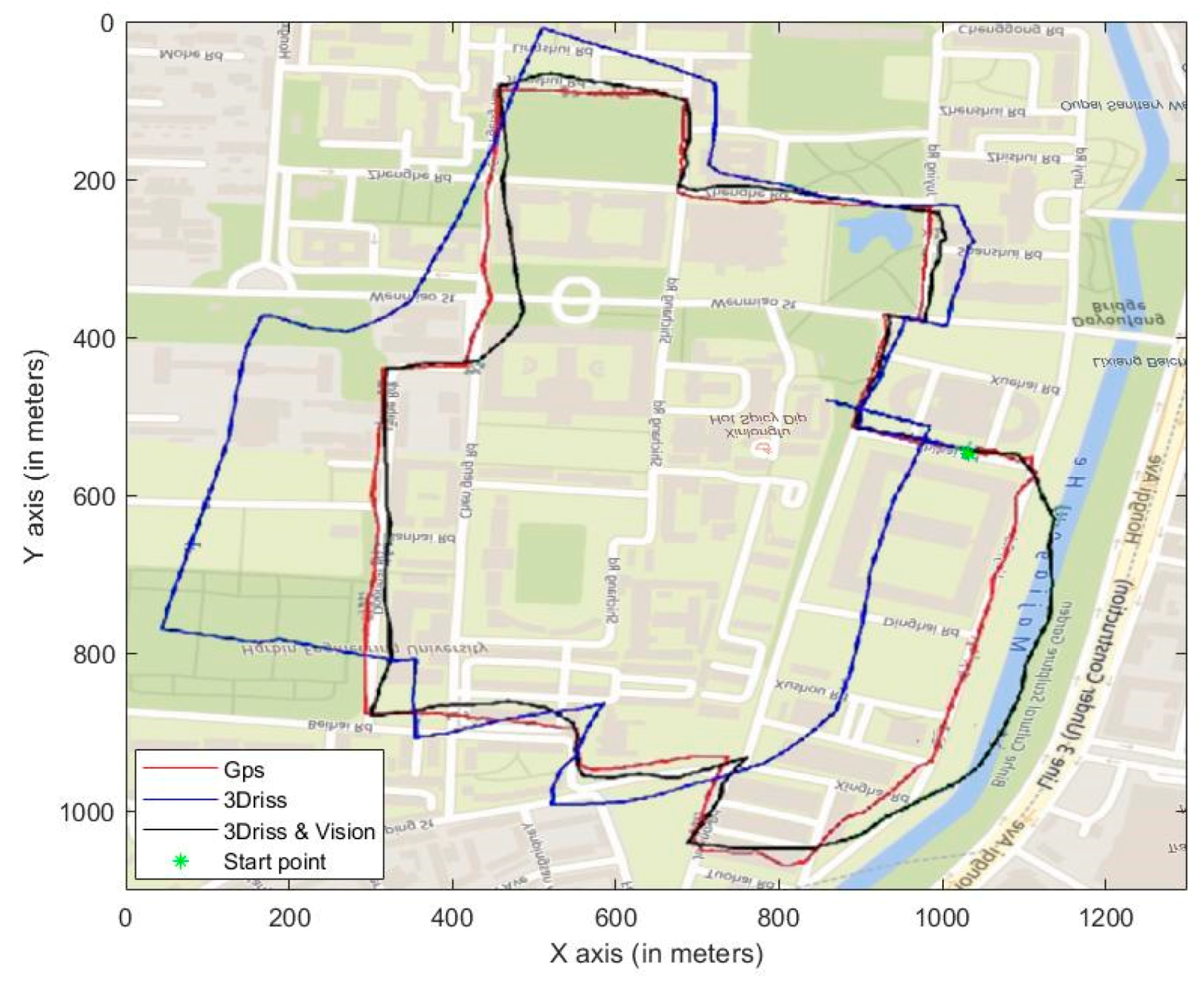
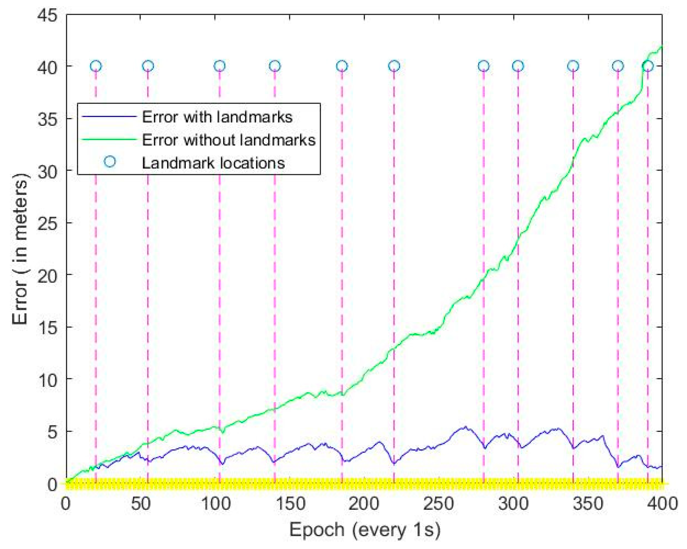
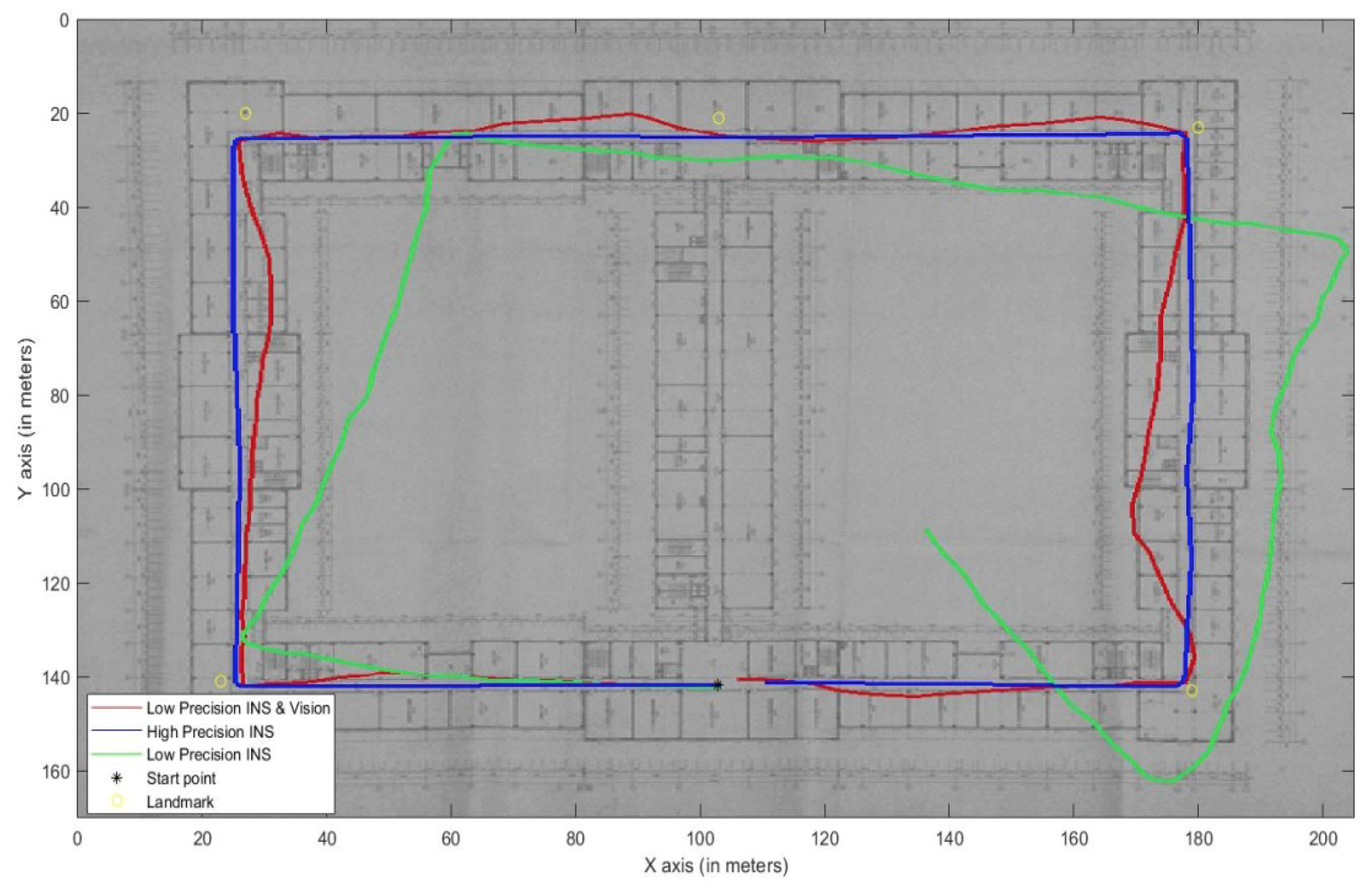
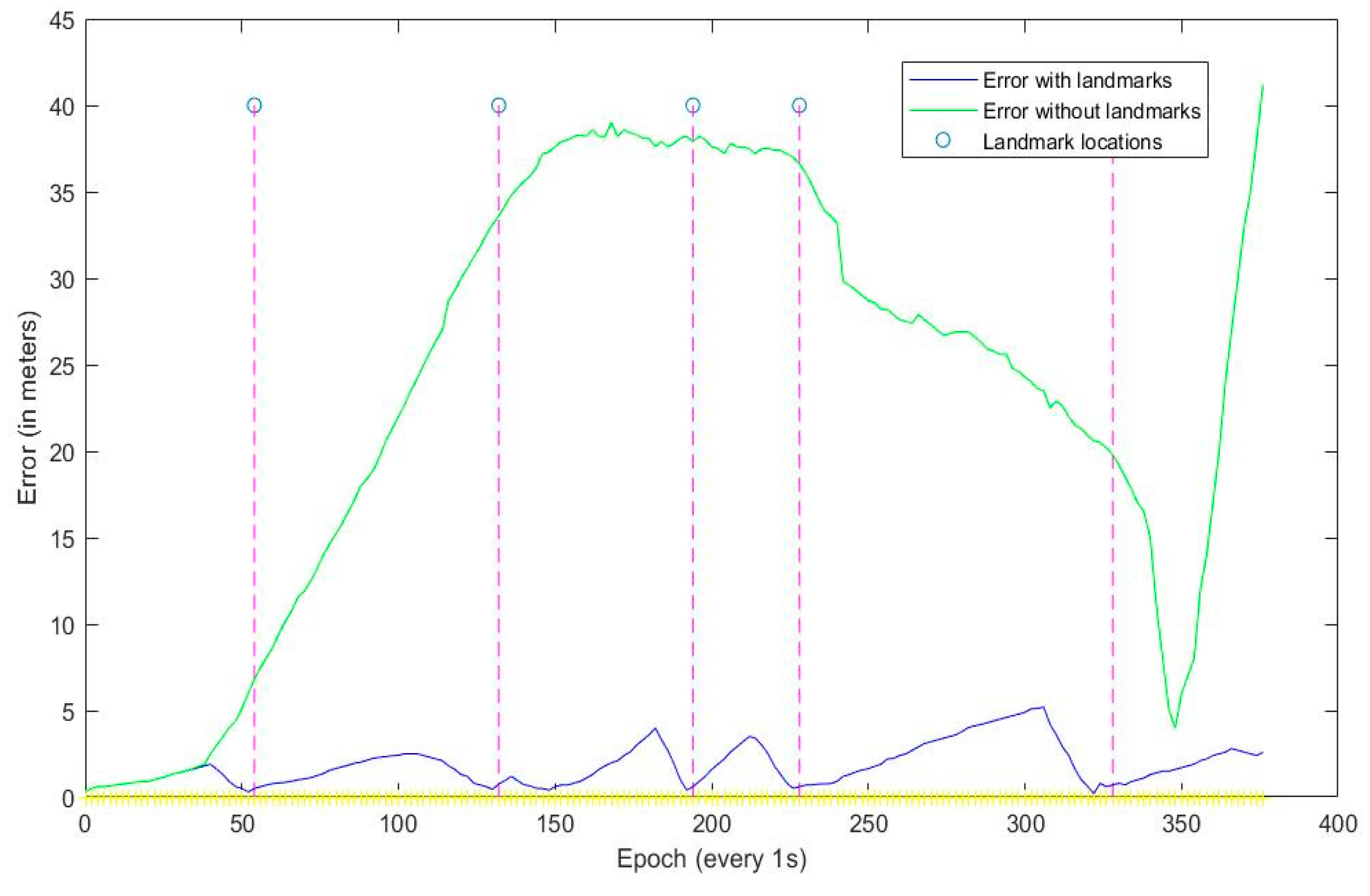
By using landmarks at known positions, a feasible and accurate vehicular navigation solution was proposed for challenging the situations where GPS signal is not available over extended periods of time. Specifically, the template matching technology was utilized to detect the presence of the landmarks, and every time a landmark was detected, the location and azimuth angle of the vehicle was fed into an EKF. By using this method, over most of an indoor trajectory, the vehicular position was accurately estimated to be within the range of the map. This study revealed that the proposed integration of the 3D-RISS/MLEVD could provide the accurate location information. Moreover, the proposed 3D-RISS/MLEVD vehicular navigation technology was conducted by an outdoor experiment the high-precision GPS positioning only used as a benchmark.

Results showed that the trajectory provided by the visual/inertial integrated navigation system is closer to the referenced GPS trajectory than the trajectory provided by inertial navigation alone. Through the indoor experiment, a set of low-cost and low-precision INS with visual can achieve the precision of high-precision INS in challenging environments such as in outdoor satellite signal outage occasions or in indoor environment. By incorporating machine learning, the system could capture the landmark information more quickly and accurately, which increases its potential for real-time positioning application. The advantages of this system are low-cost, high-accuracy and suitable for environments without GPS and simple operation. However, one of its disadvantages is that it needs a lot of preliminary work such as setting landmarks and getting their information. Another disadvantage is the light intensity sometimes would influence the visual positioning effect, which could be compensated by collecting large amounts of data under different lighting conditions.

References

1. Misra, P.; Enge, P. Global Positioning System: Signals, Measurements, and Performance; Ganga-Jamuna Press: Lincoln, MA, USA, 2011. [Google Scholar]
2. Nerem, R.S.; Larson, K.M. Global Positioning System, Theory and Practice. Eos Trans. Am. Geophys. Union 2001, 82, 365. [Google Scholar] [CrossRef]
3. Titterton, D.; Weston, J. Strapdown Inertial Navigation Technology; The Institution of Electrical Engineers: London, UK, 2004. [Google Scholar]
4. Mainone, M.; Cheng, Y.; Matthies, L. Two years of visual odometer on the mars exploration rovers. J. Field Robot. Spec. Issue Space Robot. 2007, 24, 169–186. [Google Scholar] [CrossRef] [Green Version]
5. Zhong, Z.; Yi, J.; Zhao, D. Novel approach for mobile robot localization using monocular vision. Proc. SPIE 2003, 5286, 159–162. [Google Scholar]
6. Sun, Y.; Rahman, M. Integrating Vision Based Navigation with INS and GPS for Land Vehicle Navigation in Challenging GNSS Environments. In Proceedings of the 29th International Technical Meeting of the Satellite Division of The Institute of Navigation, Portland, OR, USA, 12–16 September 2016. [Google Scholar]
7. Martinelli, A.; Siegwart, R. Vision and IMU Data Fusion: Closed-Form Determination of the Absolute Scale, Speed, and Attitude. In Handbook of Intelligent Vehicles; Springer: London, UK, 2012; pp. 1335–1354. [Google Scholar]
8. Wang, W. Research of Ego-Positioning for Micro Air Vehicles Based on Monocular Vision and Inertial Measurement. J. Jilin Univ. 2016, 34, 774–780. [Google Scholar]
9. Zhao, S.; Lin, F.; Peng, K. Vision-aided Estimation of Attitude, Velocity, and Inertial Measurement Bias for UAV Stabilization. J. Intell. Robot. Syst. 2016, 81, 531–549. [Google Scholar] [CrossRef]
10. Schmidhuber, J. Deep Learning in Neural Networks: An Overview. Neural Netw. 2015, 61, 85–117. [Google Scholar] [CrossRef] [Green Version]
11. Mnih, V.; Heess, N.; Graves, A. Recurrent Models of Visual Attention. In Proceedings of the NIPS’14: 27th International Conference on Neural Information Processing Systems, Montreal, QC, Canada, 8–13 December 2014. [Google Scholar]
12. Karpathy, A.; Joulin, A.; Li, F. Deep Fragment Embeddings for Bidirectional Image Sentence Mapping. In Proceedings of the International Conference on Neural Information Processing Systems, Montreal, QC, Canada, 8–13 December 2014; MIT Press: Cambridge, MA, USA, 2014. [Google Scholar]
13. Goodfellow, I.J.; Bulatov, Y.; Ibarz, J. Multi-digit Number Recognition from Street View Imagery using Deep Convolutional Neural Networks. arXiv 2013, arXiv:1312.6082. [Google Scholar]
14. Vinyals, O.; Toshev, A.; Bengio, S. Show and Tell: A Neural Image Caption Generator. In Proceedings of the IEEE Conference on Computer Vision and Pattern Recognition, San Juan, PR, USA, 17–19 June 1997. [Google Scholar]
15. Krizhevsky, A.; Sutskever, I.; Hinton, G. ImageNet Classification with Deep Convolutional Neural Networks, NIPS; Curran Associates Inc.: Red Hook, NY, USA, 2012. [Google Scholar]
16. Lecun, Y.; Bengio, Y.; Hinton, G. Deep learning. Nature 2015, 521, 436. [Google Scholar] [CrossRef]
17. Wu, M.; Gao, Y.; Jung, A. The Actor-Dueling-Critic Method for Reinforcement Learning. Sensors 2019, 19, 1547. [Google Scholar] [CrossRef] [Green Version]
18. Tai, L.; Li, S.; Liu, M. A deep-network solution towards model-less obstacle avoidance. In Proceedings of the IEEE/RSJ International Conference on Intelligent Robots and Systems (IROS 2016), Daejeon, Korea, 9–14 October 2016. [Google Scholar]
19. Mirowski, P.; Grimes, M.K.; Malinowski, M. Learning to Navigate in Cities Without a Map. arXiv 2013, arXiv:1804.00168. [Google Scholar]
20. Zhu, Y.; Mottaghi, R.; Kolve, E. Target-driven visual navigation in indoor scenes using deep reinforcement learnin. In Proceedings of the 2017 IEEE International Conference on Robotics and Automation (ICRA), Singapore, 29 May–3 June 2017. [Google Scholar]
21. Hinton, G.E. Rectified Linear Units Improve Restricted Boltzmann Machines Vinod Nair. In Proceedings of the International Conference on International Conference on Machine Learning, Haifa, Israel, 21–24 June 2010; Omnipress: Paraskevi, Greece, 2010. [Google Scholar]
22. Russakovsky, O.; Deng, J.; Su, H. Image Net Large Scale Visual Recognition Challenge. Int. J. Comput. Vis. 2015, 115, 211–252. [Google Scholar] [CrossRef] [Green Version]
23. Bell, R.M.; Koren, Y. Lessons from the Netflix prize challenge. ACM SIGKDD Explor. Newsl. 2007, 9, 75. [Google Scholar] [CrossRef]
24. Zhang, Z. A flexible new technique for camera calibration. IEEE Trans. Pattern Anal. Mach. Intell. 2000, 22, 1330–1334. [Google Scholar] [CrossRef] [Green Version]
25. Liu, L.; Liu, M.; Shi, Y. Correction method of image distortion of fisheye lens. Infrared Laser Eng. 2019, 48, 272–279. [Google Scholar]
26. Sutton, M.A.; Orteu, J.J.; Schreier, H. Image Correlation for Shape, Motion and Deformation Measurements: Basic Concepts, Theory and Applications; Springer Science & Business Media: Berlin, Germany, 2009. [Google Scholar]
27. Loevsky, I.; Shimshoni, I. Reliable and efficient landmark-based localization for mobile robots. Rob. Auton. Syst. 2010, 58, 520–528. [Google Scholar] [CrossRef]
28. Noureldin, A.; Karamat, T.B.; Georgy, J. Fundamentals of Inertial Navigation, Satellite-Based Positioning and Their Integration; Springer: New York, NY, USA, 2013. [Google Scholar]
29. Iqbal, U.; Okou, F.; Noureldin, A. An Integrated Reduced Inertial Sensor System-RISS/GPS for Land Vehicles. In Proceedings of the IEEE/ION Position, Location and Navigation Symposium, Monterey, CA, USA, 5–8 May 2008. [Google Scholar]
30. Georgy, J.; Noureldin, A.; Korenberg, M.J.; Bayoumi, M.M. Low-cost three-dimensional navigation solution for RISS/GPS integration using mixture particle filter. IEEE Trans. Veh. Technol. 2010, 59, 599–615. [Google Scholar] [CrossRef]
31. Chang, T.; Wang, L.; Chang, F. A solution to the ill-conditioned GPS positioning problem in an urban environment. IEEE Trans. Intell. Trans. Syst. 2009, 10, 135–145. [Google Scholar] [CrossRef]
32. Li, Q.; Chen, L.; Li, M. A sensor-fusion drivable-region and lane-detection system for autonomous vehicle navigation in challenging road scenarios. IEEE Trans. Veh. Technol. 2014, 63, 540–555. [Google Scholar] [CrossRef]
33. Rose, C.; Britt, J.; Allen, J. An integrated vehicle navigation system utilizing lane-detection and lateral position estimation systems in difficult environments for GPS. IEEE Trans. Intell. Trans. Syst. 2014, 15, 2615–2629. [Google Scholar] [CrossRef]
34. Karamat, T.B.; Atia, M.M.; Noureldin, A. Performance Analysis of Code-Phase-Based Relative GPS Position and Its Integration with Land Vehicle Motion Sensors. IEEE Sens. J. 2014, 14, 3084–3100. [Google Scholar] [CrossRef]
35. Atia, M.M.; Karamat, T.; Noureldin, A. An Enhanced 3D Multi-Sensor Integrated Navigation System for Land-Vehicles. J. Navig. 2014, 67, 651–671. [Google Scholar] [CrossRef]
36. Gelb, A. Applied Optimal Estimation; M.I.T. Press: Cambridge, MA, USA, 1974. [Google Scholar]
37. Navigation and Monitoring. Available online: http://en.flag-ship.cn/product-item-3.html (accessed on 2 July 2015).
38. Simonyan, K.; Andrew, Z. Very deep convolutional networks for large-scale image recognition. arXiv 2014, arXiv:1409.1556, 1409–1556. [Google Scholar]
39. MPU-9250 Register Map and Descriptions. Available online: https://wenku.baidu.com/view/6350b62babea998fcc22bcd126fff705cc175cc4.html (accessed on 8 June 2013).
Figure 1. Camera calibration board.
Electronics 09 00193 g001
Figure 2. Original image and the image after correcting distortion. (a) Original; (b) Correcting Distortion.
Electronics 09 00193 g002
Figure 3. Landmark in 6-m image and 7-m image.
Electronics 09 00193 g003
Figure 4. Schematic diagram of 3D-RISS mechanization.
Electronics 09 00193 g004
Figure 5. Block diagram of the 3D-RISS/MLEVD integrated navigation system.
Electronics 09 00193 g005
Figure 6. Experimental equipment.
Electronics 09 00193 g006
Figure 7. Architecture of the neural network.
Electronics 09 00193 g007
Figure 8. Training result.
Electronics 09 00193 g008
Figure 9. Example of a landmark.
Electronics 09 00193 g009
Figure 10. Six matching techniques at time 10:47:16.
Electronics 09 00193 g010
Figure 11. Landmark detection methods at time 10:47:17.
Electronics 09 00193 g011
Figure 12. The trajectory comparison of the 3D-RISS and the 3D-RISS/Vision.
Electronics 09 00193 g012
Figure 13. Single-point error of outdoor experiment.
Electronics 09 00193 g013
Figure 14. Experimental equipment.
Electronics 09 00193 g014
Figure 15. experimental results.
Electronics 09 00193 g015
Figure 16. Single-point error of indoor experiment.
Electronics 09 00193 g016