Leukemia Image Segmentation Using a Hybrid Histogram-Based Soft Covering Rough K-Means Clustering Algorithm

Abstract

Segmenting an image of a nucleus is one of the most essential tasks in a leukemia diagnostic system. Accurate and rapid segmentation methods help the physicians identify the diseases and provide better treatment at the appropriate time. Recently, hybrid clustering algorithms have started being widely used for image segmentation in medical image processing. In this article, a novel hybrid histogram-based soft covering rough k-means clustering (HSCRKM) algorithm for leukemia nucleus image segmentation is discussed. This algorithm combines the strengths of a soft covering rough set and rough k-means clustering. The histogram method was utilized to identify the number of clusters to avoid random initialization. Different types of features such as gray level co-occurrence matrix (GLCM), color, and shape-based features were extracted from the segmented image of the nucleus. Machine learning prediction algorithms were applied to classify the cancerous and non-cancerous cells. The proposed strategy is compared with an existing clustering algorithm, and the efficiency is evaluated based on the prediction metrics. The experimental results show that the HSCRKM method efficiently segments the nucleus, and it is also inferred that logistic regression and neural network perform better than other prediction algorithms.

1. Introduction

Due to the growth of advanced medical imaging modalities, it is very difficult to analyze the medical images manually. For this reason, an advanced and efficient computer-aided system is needed to diagnose the diseases. This will help the hematologist to begin the treatment at the right time and increase the patient’s survival rate. Leukemia is a cancer of blood-forming tissues that affects the bone marrow. Leukemia is caused by the proliferation of abnormal white blood cells in the body. Leukemia is mostly affected by people living in developed countries and children aged 14 or under. As per the National Cancer Institute (NCI) statistics, in the United States, it is expected that there will be 62,130 persons as new cases for cancer treatment and 245,000 cases that are fatal or very serious [1]. In India, leukemia stands at ninth position among diseases (tumors) among children [2,3]. Leukemia is identified into two broad categories such as acute and chronic. Acute forms of leukemia occur when the number of immature blood cells increases, and it is the most common type of leukemia in children. Segmenting an image of a nucleus is one of the major challenging tasks in leukemia diagnosis. Recently, soft computing plays an important role in many research areas such as medical image processing, pattern recognition, big data analytics, Internet of Things (IoT) analysis, bioinformatics, and so on.

The rough set theory [4] was proposed by Pawlak in 1982. This concept is an extension of set theory for the study of intelligent systems characterized by insufficient and incomplete information. This classical rough set theory is based on equivalence relations, but it can also be extended to covering based rough sets [5,6,7]. In 1999, Molodtsov [8] proposed the concept of a soft set, which can be seen as a new mathematical approach to vagueness. The absence of any restrictions on the approximate description in soft set theory makes this theory very versatile and easily applicable in practice. Maji et al. [9] improved Molodtsov’s idea by introducing several operations in soft set theory. In [10], the researcher investigated a soft covering-based rough set as a new kind of soft rough set. This method is a combination of a covering soft set and rough set. In [11], a covering-based rough k-means clustering approach is applied to segment the leukemia nucleus. The advantage of covering-based subsets is that they generate upper and lower approximations by using the covering feature, which brings about more roughness. Since different clusters give rise to different results, determination of the number of clusters is a difficult task in clustering-based segmentation. To overcome this limitation, the hybrid histogram-based soft covering rough k-means clustering algorithm (HSCRKM) is introduced to segment the image of the leukemia nucleus. In this algorithm, the peak values of the histogram of an image are identified and the number of clusters is initialized. This will avoid the random initialization of a number of clusters. Here, soft covering approximation space is also included. The term ‘covering soft set’ is more accurate than ‘soft rough set.’ It also combines the strengths of covering soft set theory and the rough k-means clustering algorithm to effectively segment the image of the nucleus. Soft covering rough approximation is utilized to find the lower and upper approximation values. The performance of the HSCRKM algorithm is evaluated using existing algorithms such as k-means clustering, fuzzy c-means clustering, and particle swarm optimization (PSO)-based clustering. Different types of features such as GLCM-0, GLCM-45, GLCM-90, GLCM-135, and shape color-based features are extracted from the segmented leukemia nucleus image. Nowadays, a lot of machine learning algorithms are applied to predict the degree of sickness. The state-of-art machine learning prediction algorithms such as neural networks (NN) [12], logistic regression (LR) [13], support vector machine (SVM) [14], naive Bayes (NB) [15], k-nearest neighborhood (KNN) [13], decision tree (DT) [13], and random forest (RF) [16] are applied to classify the cancerous and non-cancerous leukemia cells. The empirical results show that logistic regression and neural network efficiently predict the blast and non-blast cells when compared with other prediction algorithms.

The main objective of this research work is to develop a diagnostic approach for the identification of acute lymphoblastic leukemia blast cells using image processing and computational intelligence techniques. In experimental analysis, relevant image processing and computational intelligence techniques are applied in order to select the most suitable approach for the delineation of acute lymphoblastic leukemia cells. The following objectives have been formulated in order to predict leukemia: to apply computational intelligence-based algorithms for the segmentation of acute lymphoblastic leukemia blast cells in images and to apply machine learning algorithms to evaluate the performance of the proposed method.

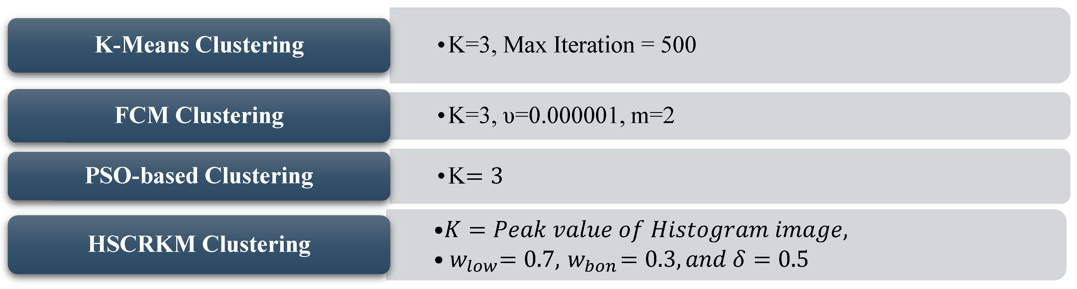
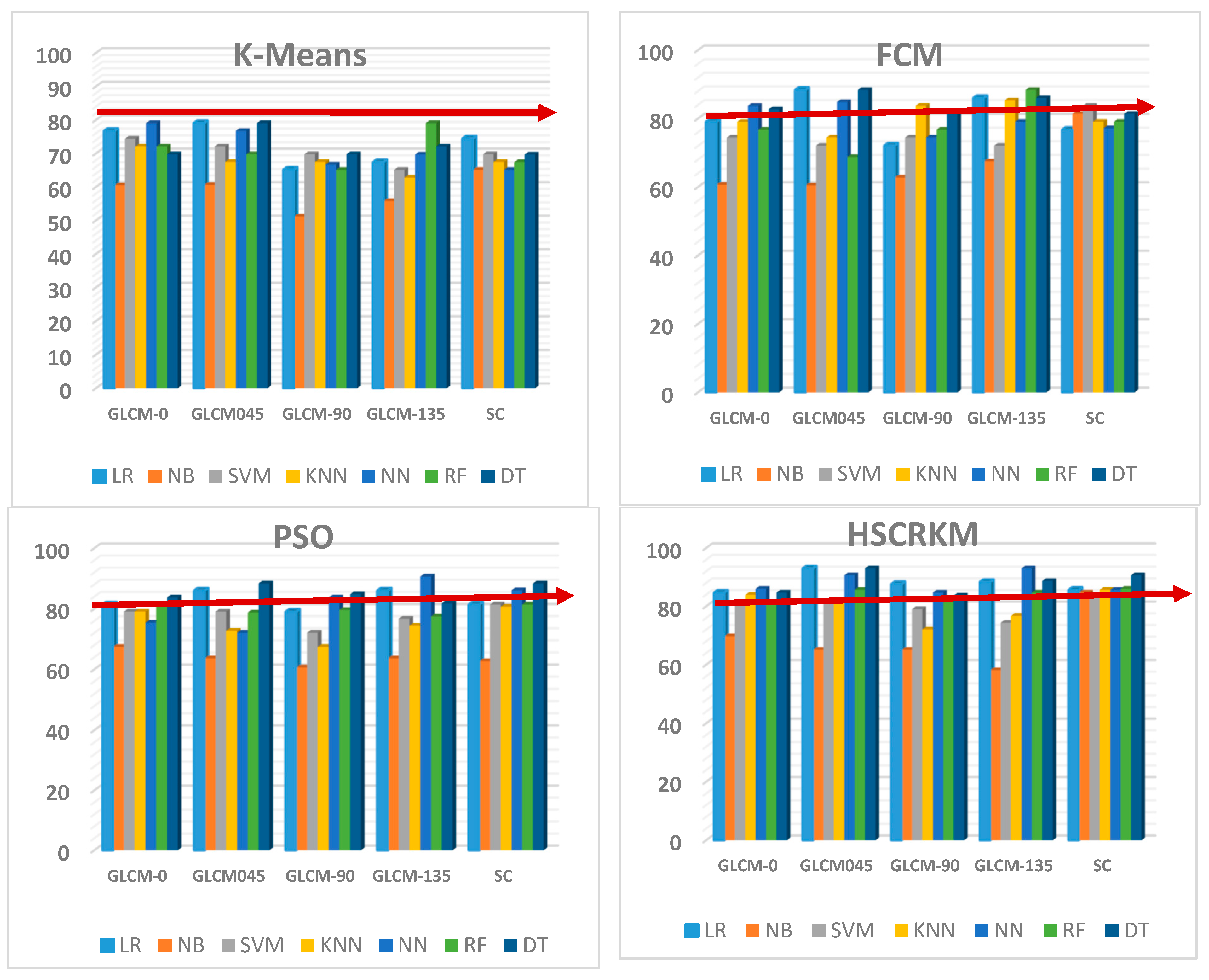
The contribution of this study is summarized as follows. To find the number of clusters using the peak value of a histogram image and compute the lower and upper approximation values based on the soft covering approximation space, three clustering methods—k-means, FCM, and PSO-based clustering—are preferred for segmentation comparison. Through these methods, different kinds of features are extracted, and the efficiency of the proposed algorithm is assessed using machine learning prediction algorithms. The HSCRKM achieves the successful results i.e., above 80% when compared with the existing clustering algorithms. Therefore, it can be concluded that the HSCRKM clustering algorithm works effectively with the other clustering algorithms.

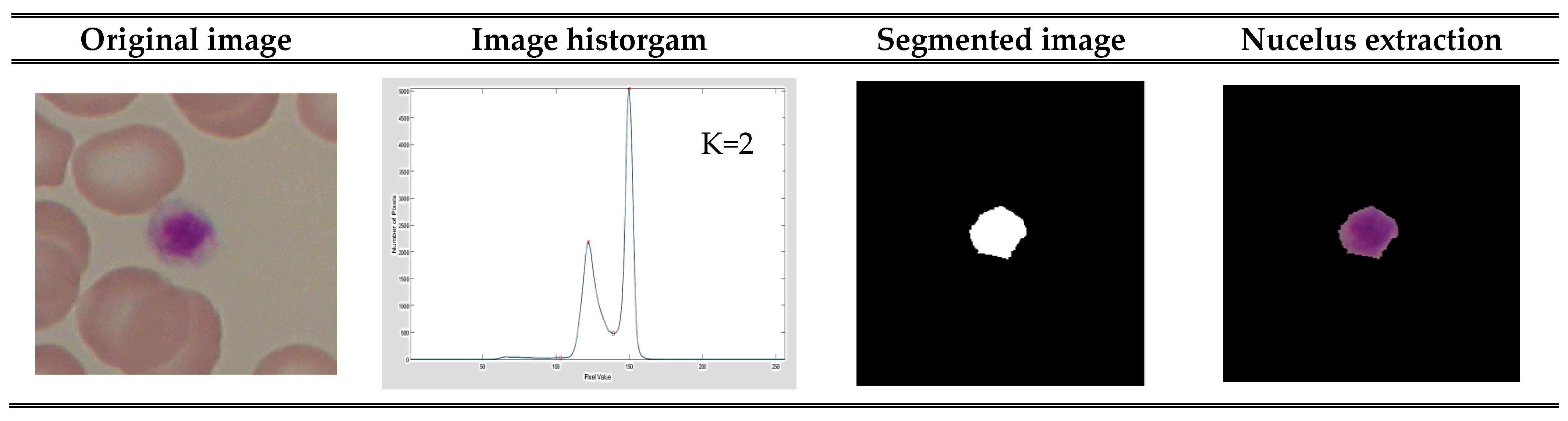
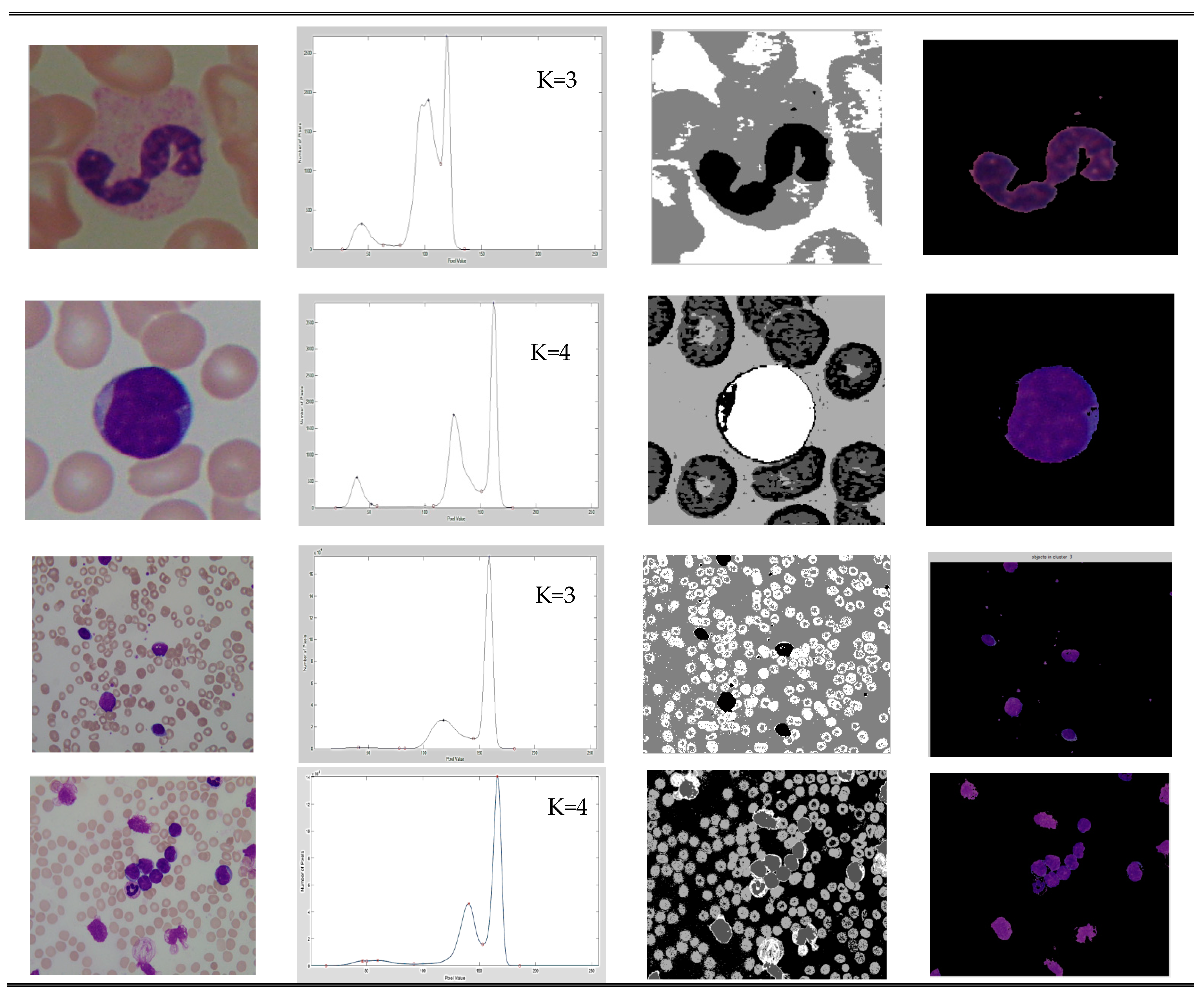
In the clustering algorithm, defining the number of clusters is a very difficult task. To overcome this limitation, the proposed algorithm identifies the peak values of the histogram of an image and initializes the number of clusters. This is one of the advantages of our proposed method, which avoids the random initialization of a number of clusters. The next advantage of the HSCRKM algorithm is that it combines the strengths of covering soft set theory and the rough k-means clustering algorithm to effectively segment the image of the nucleus. Based on a literature review, the term ‘covering soft set’ is more accurate than ‘soft rough set’, since it gives a better result than the soft rough set for several applications. In covering rough sets, the lower and upper approximation values are computed based on the soft covering approximation space.

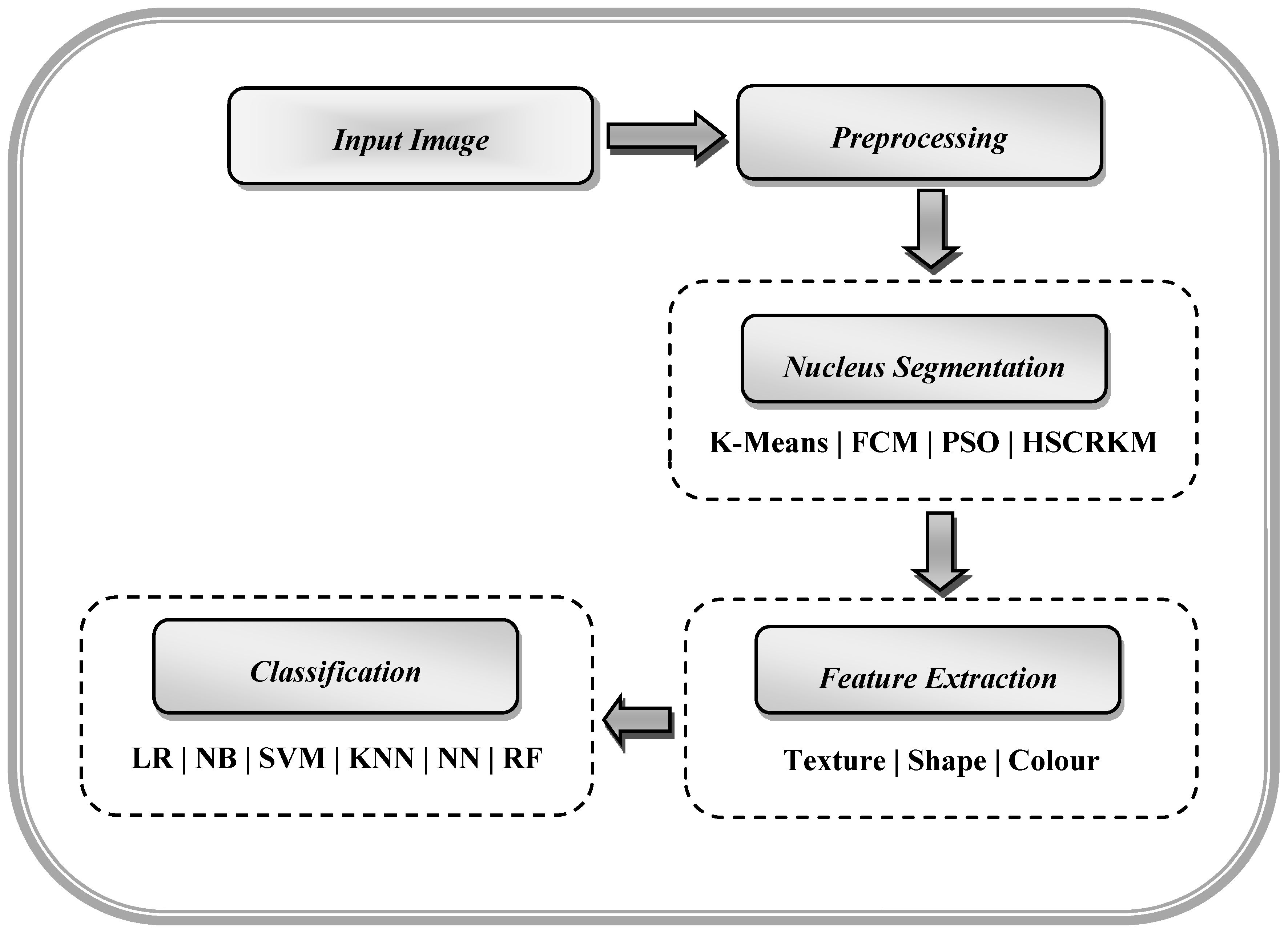
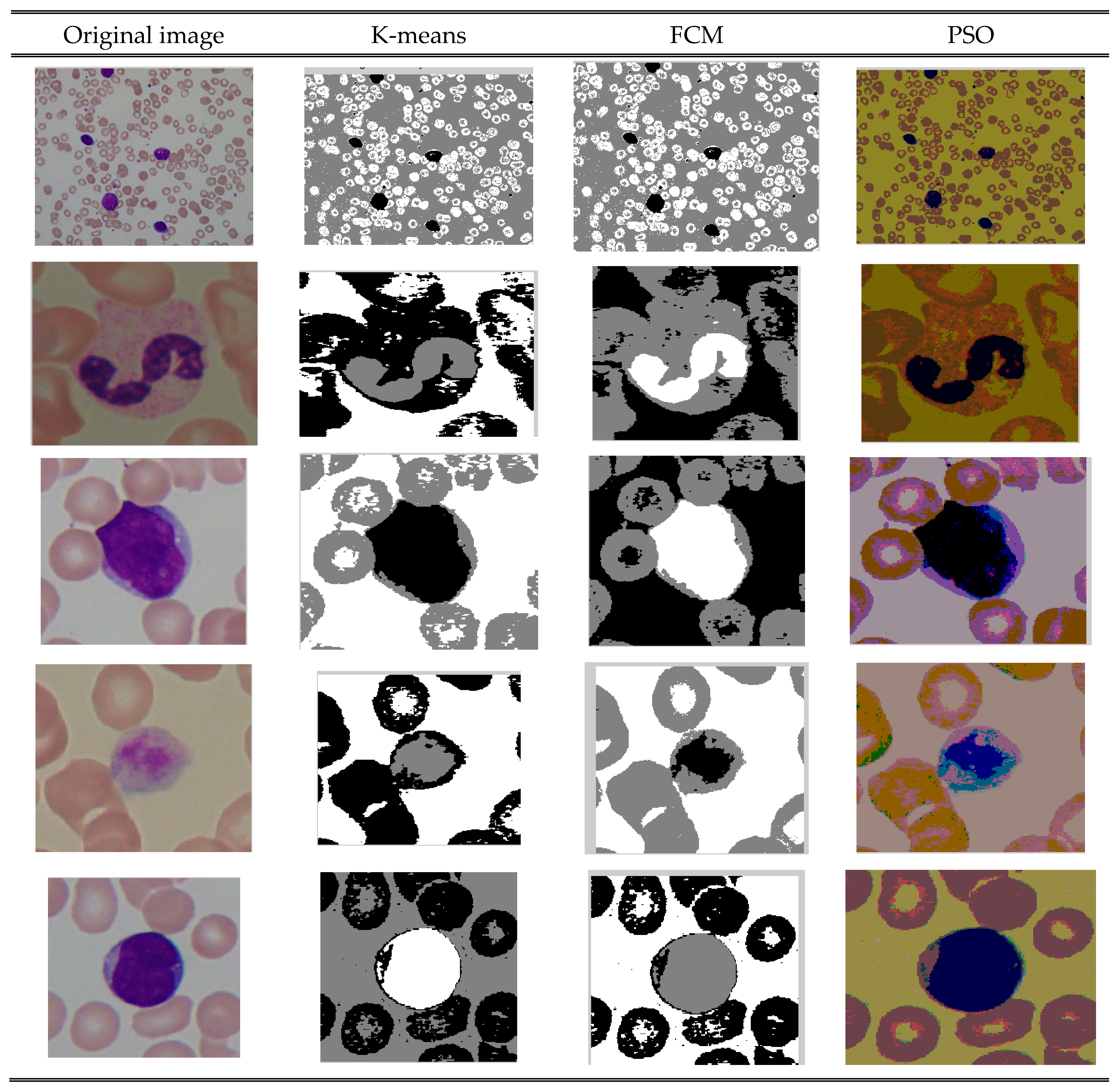
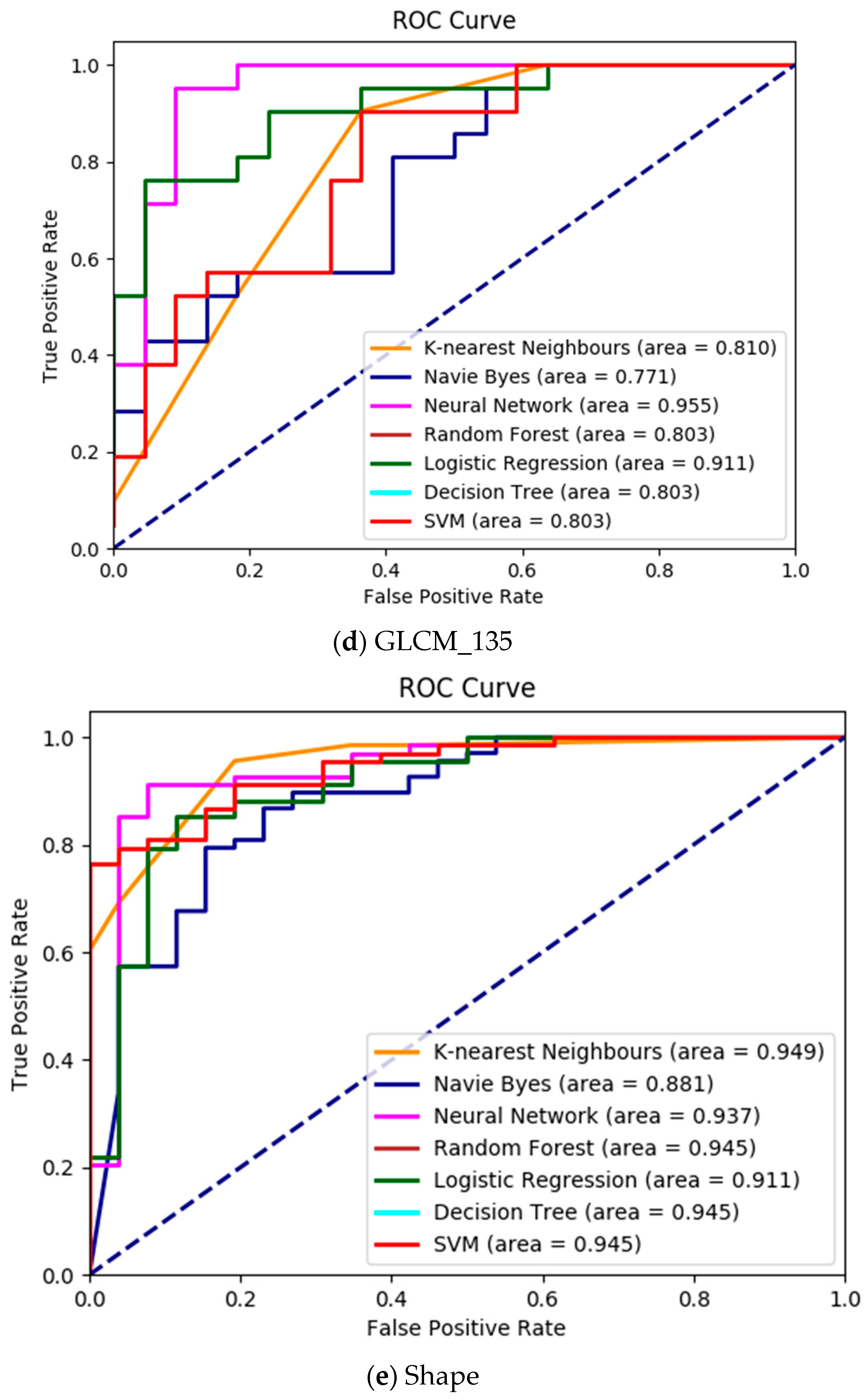
Morphologically, a lymphoblast consists of a massive nucleus of irregular shape and size. In blood sample images, it is difficult to identify the cytoplasm, because it appears rarely and even if it does, it looks intensely colored. The nucleus and cytoplasm of lymphoblast cells reflect the morphological and functional changes. Feature extraction plays a main role in the assessment of leukemia in blood samples. After segmenting the nucleus using the proposed HSCRKM algorithm, salient features are extracted. It reduces the amount of data space and the working time of an image. In this research, different kinds of features are extracted such as gray level co-occurrence matrix (GLCM), color, and shape-based features. These were measured from every channel of the segmented nucleus image. The efficiency of the proposed algorithm is assessed using machine learning prediction algorithms. The performance of the segmentation algorithms was analyzed in the light of different machine learning (ML) prediction methods. With respect to HSCRKM clustering algorithms, most of the ML methods (except naive Bayes) achieved greater than 80% prediction accuracy compared with the existing clustering algorithms, viz., k-means clustering, fuzzy c-means clustering, and rough k-means clustering. It is inferred that the proposed clustering algorithms are more effective in segmenting the nucleus image. Due to the effective segmentation process, the extracted features have increased the prediction accuracy. To evaluate the experimental results, we have empirically set the best accuracy to be greater than 80%. The outline of the proposed system is shown in Figure 1.

The rest of the research report is organized as follows. Section 2 reviews the related literature on clustering-based segmentation algorithms. Section 3 describes the methods of the proposed algorithm and its results. The empirical results are discussed in Section 4. Section 5 states the conclusion and indicates the future direction of this research.

2. Related Literature

In recent years, a lot of clustering algorithms have been developed for segmenting medical images.

Petal [17] applied k-means clustering for segmentation and the Zack algorithm for clustered white blood cells (WBCs). The features—namely, the mean, standard deviation, area, elongation, perimeter, color etc.—are extracted, and support vector machine (SVM) was used to classify the cells. The proposed algorithm effectively segmented the WBCs, which produced 93.57% accuracy. For this experiment, 27 images from the Acute Lymphoblastic Leukemia Image Database (ALL-IDB) were utilized.

Two bare-bones particle swarm optimization (BBPSO) algorithms with and without subswarms were introduced by Srisukkham et al. in 2017 [18] to diagnosis the leukemia cells. A stimulating discriminant measure (SDM)-based clustering algorithm that combined with the genetic algorithm (GA) was employed to segment the nucleus, cytoplasm, and background regions. The relevant features were extracted; then, various feature selection methods such as particle swarm optimization (PSO), cuckoo search (CS), and dragonfly algorithm (DA) were applied to select the optimal features and reduce the dimensions. An average geometric mean was computed with different sizes of training and test samples to evaluate the performance of the proposed methods. The BBPSO and binary BBPSO algorithms produced 91% to 96% of the geometric mean value.

Su [19] developed two stages of segmentation process using k-means clustering and HMRF (hidden Markov random field), which are used to group the six different types of AML cells from the bone marrow images. The segmentation algorithm achieved an accuracy of 96% to 98% (average) when compared with other existing segmentation methods.

In [20], k-means and fuzzy c-means clustering algorithms were applied to segment the brain tumor images. Various feature reduction algorithms, namely probabilistic principal component analysis (PPCA), expectation maximization-based principal component analysis (EM-PCA), the generalized Hebbian algorithm (GHA), and adaptive principal component extraction (APEX) were employed to reduce the dimensions of the feature set. The produced coefficient of variance (CV) values for k-means and Fuzzy C-mean (FCM) are 0.4582 and 0.1224, respectively.

In [21], potential field segmentation was employed to segment the MRI brain tumor images. This method achieved the standard deviation of 0.283, the average value of 0.517, and the median values of 0.644. From the experimental results, it was observed that ensemble methods generated better segmentations.

Küçükkülahlı [22] and Namburu [23] identified the number of cluster values in the clustering algorithm using the peak value of the histogram of an image. In [22], the automatic segmentation method using the histogram-based k-means clustering algorithm was developed. In [23], the soft fuzzy rough c-means clustering algorithm (SFRCM) was used to segment the MRI brain tumor images. The proposed SRFCM algorithm achieved a better Jaccard coefficient value of 0.97 for without noise and 0.79 for with 9% Gaussian noise when compared with the existing clustering algorithms namely, k-means, rough k-means (RKM), rough fuzzy c-means (RFCM), and generalized rough c-means (GFCM).

Ali [24] introduced a new clustering algorithm based on neutrosophic orthogonal matrices (CANOM) to segment the dental X-ray images. The experimental results show that the CANOM simplified silhouette width criterion (SSWC) index is 0.941 and the FCM is 0.02. CANOM is also better than Otsu and eSFCM with the values being 0.657 and 0.647, respectively. The value of CANOM is 47 times larger than that of FCM and 1.43 times larger than those of Otsu and eSFCM.

In [25], the unsupervised fuzzy c-means (FCM) clustering technique was employed for prostate cancer MRI images. The derived average dice similarity, Jaccard index, sensitivity, specificity, mean absolute difference, and Hausdorff distance is 88.68, 81.26, 90.71, 88.09, 88.09, 3.5, and 4.1 respectively.

In [26], the proposed multi-Otsu thresholding-based segmentation method can successfully segmented the CT image stacks. In addition, it sows the distribution characteristics of different components in three dimensions.

In [27], the enhanced adaptive fuzzy k-means (AFKM) algorithm was used to detect the three regions such as white matter (WM), gray matter (GM), and cerebrospinal fluid spaces (CSF) in the brain images. AFKM performed better than FCM, which produced a minimum mean square error (MSE) value of 2.2441.

In [28], the clustering method intuitionistic fuzzy c-means (IFCM) was applied for medical image segmentation. It is observed from the experimental results that the proposed method outperformed other algorithms that achieved the average quantitative index 0.95. The chronic wound region was detected using fuzzy spectral clustering in [29]. The proposed method produced 91.5% segmentation accuracy, an 86.7% Dice index, a Jaccard score of 79.0%, 87.3% sensitivity, and 95.7% specificity.

In [30], the convolutional neural networks (CNN) approach is applied to identify the subtypes of leukemia. It is observed from the experimental results that the CNN model achieves 88.25% and 81.74% accuracy for leukemia and healthy cells, respectively. From the literature review, it is inferred that the clustering-based algorithms were applied to segment the tumor region. A brief review of the literature on various clustering methods in image segmentation and their performances appears in

Table 1. Overview of the literature on clustering algorithms.

Author	Used Methods	Objective	Type of Diseases	Imaging Modalities/Dataset Used	No. of IMAGES	Performance Metrics and Accuracy %
Patel et al., 2015 [17]	K-mean clustering Zack algorithm, Support vector machines (SVM)	The K-means clustering algorithm was used to detect the white blood cells and the Zack algorithm was applied to categorize the cells.	Leukemia	Microscopic image (ALL-IDB)	27	Classification accuracy 93.57%
Srisukkham et al., 2017 [18]	Spatial Data Mining (SDM)-based clustering, Genetic Algorithm (GA), particle swarm optimization (PSO), Bare Bones PSO (BBPSO)	This optimization method was utilized to diagnose leukemia.	Acute lymphoblastic leukemia (ALL)	Microscopic image (ALL-IDB)	180	Geometric mean 91 to 96%
Su et al., 2017 [19]	K-means, Hidden Markov random field	This algorithm segmented the nucleus from the background, extracted the features, and then classified the blast cells.	Acute myeloid leukemia	Microscopic image (AML Patient)	61	Segmentation accuracy 96 to 98% (average)
Kaya et al., 2017 [20]	K-means, fuzzy c-means	Comparative analysis of various types of PCA algorithms on MRIs for two cluster methods.	Brain tumor	MRI (Hospital)	-	Average reconstruction error rates, Euclidean distance error rate, CV of K-Means = 0.4582 FCM = 0.1224
Cabria et al., 2017 [21]	Potential field clustering	The algorithm is based on an analogy with the concept of potential field in physics and views the intensity of a pixel in an MRI as a “mass” that creates a potential field.	Brain tumor	MRI (BRATS)	30	SD = 0.283, Average = 0.517, Median = 0.644.
Küçükkülahlı et al., 2016 [22]	Histogram-based k-means clustering	This method to find the optimum cluster number based on the histogram of an image.	MATLAB media	Image Dataset	10-15	Derived metrics
Ali et al., 2017 [23]	Fuzzy clustering based on neutrosophic orthogonal matrix	This algorithm transforms image data into a neutrosophic set and computes the inner products of the cutting matrix of input. Then, pixels are segmented using the orthogonal principle to form clusters.	Dental	X-Ray (Hospital)	22	DB index Silhouette index = 0.941
Rundo et al., 2018 [24]	Fuzzy c-means (FCM)	This approach automatically segments the prostate and image computes the gland volume.	Prostate cancer	MRI (Hospital)	7 (Patients)	Dice Similarity = 88.68, Jaccard index = 81.26, Sensitivity = 90.71, Specificity = 88.09, Mean Absolute Difference = 3.5, Hausdorff distance = 4.1
Zhang et al., 2017 [25]	Multi-Otsu thresholding algorithm	This segmentation method can successfully segment CT image stacks. In addition, it sows the distribution characteristics of different components in three dimensions.	Backscattered electron images	X-ray CT (Hospital)	1571 (Slice)	Derived metrics
Namburu et al., 2017 [26]	classical k-means (KM), rough k-means (RKM), rough fuzzy c-means (RFCM), and generalized rough c-means (GFCM).	In this method, soft fuzzy rough approximations are applied to obtain the rough regions of an image and compute the similarity of the clusters using soft set similarity coefficient.	Brain tumor	MRI (BRATS)	20	Jaccard’s coefficient = 0.97 Accuracy
Ganesh et al., 2017 [27]	Enhanced adaptive fuzzy k-means algorithm	This approach is used to classify the three important regions in brain: namely, white matter, gray matter, and cerebrospinal fluid spaces.	Brain tumor	MRI (Brain Image)	3	MSE 2.2441
Kaur 2017 [28]	Intuitionistic fuzzy sets-based credibilistic fuzzy c-means clustering	In this method, the hesitation factor and fuzzy entropy were utilized to improve the noise sensitivity of fuzzy c-means.	Brain tumor	MRI (brainweb)	3	Quantitative index 0.95
Dhane et al., 2017 [29]	Fuzzy spectral clustering gray-based fuzzy similarity measure	This approach is adopted to compute the ulcer boundary demarcation and estimation.	Chronic wound	Digital Camera	70	Sensitivity = 87.3% Specificity = 95.7% Accuracy = 91.5% Dice index = 86.7% Jaccard score = 79.0%
Ahmed et al., 2019 [30]	Convolutional neural network (CNN)	This approach is identify the subtypes of leukemia.	Leukemia	Microscopic image (ALL-IDB) ASH Image Bank	903	Accuracy = 88.25% (Leukemia) Accuracy = 81.74% (Healthy cell)

.

3. Methods

3.1. Basics of Soft Covering Based Rough Set

This section describes the basic properties of soft covering-based rough approximation [11].

Definition 1.

Let$C_G=\left(F,A\right)$be a covering soft set over$U$if$F\left(a\right)\ne \varnothing ,\forall a\in A$. The pair$S=\left(U,C_G\right)$is known as soft covering approximation space. For a set$X\subseteq U$, the soft covering lower and upper approximations are, respectively, defined as

$${\underset{\_}{S}}_{\ast }\left(X\right)={\cup }_{a\in A}\left\{F\left(a\right):F\left(a\right)\subseteq X\right\}$$

(1)

$${\overline{S}}^{\ast }\left(X\right)=\cup \left\{M{d}_S\left(x\right):x\in X\right\}.$$

(2)

In addition,

$$S_{pos}\left(X\right)={\underset{\_}{S}}_{\ast }\left(X\right)$$

(3)

$$S_{neg}\left(X\right)=U-{\overline{S}}^{\ast }\left(X\right)$$

(4)

$$S_{bon}\left(X\right)={\overline{S}}^{\ast }\left(X\right)-{\underset{\_}{S}}_{\ast }\left(X\right)$$

(5)

are called the soft covering positive, negative, and boundary regions of X, respectively [11].

Definition 2.

Let$S=\left(U,C_G\right)$be a soft covering approximation space. If${\overline{S}}^{\ast }\left(X\right)={\underset{\_}{S}}_{\ast }\left(X\right)$, then subset$X\subseteq U$is called soft covering. X is said to be a soft covering based rough set if${\overline{S}}^{\ast }\left(X\right)\ne {\underset{\_}{S}}_{\ast }\left(X\right)$.

The soft covering based rough set can be applied to image segmentation with the following considerations.

• The set of pixels in the input image is denoted as $U$ $U=X=\{xi/xi$ is the value of the ith pixel in the image}.
• Let $C_G=\left(F,A\right)$ be the covering soft set to be constructed containing the pixels belonging to clusters.
• The set of parameter $A$ is considered as the number of clusters ${Cl}_G\left\{i=1,2,3,\dots ,k\right\}$ to which the pixels fit.
• For example, let a set of pixels in an image be denoted as $U=\left\{x_1,x_2,x_3,x_4,\right\}$ and the parameter set $A$ be denoted as number of clusters {${Cl}_{G1}$, ${Cl}_{G2},{Cl}_{G3}$} to which the pixels belong. The distance between each pixel and the centroids are calculated. Based on the minimum distance, the pixels are grouped to the clusters. Assume that the input pixels are grouped in one cluster or more than one clusters as follows.

  $$\begin{array}{c}F\left({Cl}_{G1}\right)=\left\{x_2,x_3,x_4\right\}\\ F\left({Cl}_{G2}\right)=\left\{x_1,x_4,\right\}\\ F\left({Cl}_{G3}\right)=\left\{x_1,x_3\right\}\end{array}$$

Let (F, A) be represented as (F, A) = {F (${Cl}_G$) ∣ ${Cl}_G$ ∈ A}. The soft covering based rough set representation of the above example is given by

$$\left(F,A\right)=\left\{\begin{array}{c}{Cl}_{G1}=\left\{x_2,x_3,x_4\right\}\\ {Cl}_{G2}=\left\{x_1,x_4,\right\}\\ {Cl}_{G3}=\left\{x_1,x_3\right\}\end{array}\right\}.$$

A tabular presentation of soft sets appears in

Table 2. Soft covering-based rough set representation of an image.

U	${\mathit{C}\mathit{l}}_{\mathit{G}1}$	${\mathit{C}\mathit{l}}_{\mathit{G}2}$	${\mathit{C}\mathit{l}}_{\mathit{G}3}$
${\mathit{x}}_1$	0	1	1
${\mathit{x}}_2$	1	0	0
${\mathit{x}}_3$	1	0	1
${\mathit{x}}_4$	1	1	0

. If $x_i\in F\left({Cl}_{Gi}\right)$, then the value is one; else, it is zero.

3.2. The Proposed Histogram-Based Soft Covering Rough K-Means Clustering

The proposed histogram-based soft covering rough k-means clustering is summarized in Algorithm 1. The combination of the covering soft set and rough set gives rise to a new kind of soft rough sets. Based on the covering soft sets, soft covering rough approximation was proposed by Yüksel et al. in 2014 [11,31], which is more accurate than the soft rough set. Here, we establish a rough k-means clustering using soft covering-based rough approximation to segment the image of the leukemia nucleus. Let ${\underset{\_}{S}}_{\ast }\left(X\right)$, ${\overline{S}}^{\ast }\left(X\right)$ be denoted as soft covering lower and upper approximation, and for ${\underset{\_}{S}}_{\ast }\left(X\right)\in {\overline{S}}^{\ast }\left(X\right)i.e.$, in soft covering-based rough k-means clustering, the lower approximation is a subset of the upper approximation. The pixel data $X_n=\left(x_1,x_2,\dots \dots .x_n\right)$ of the lower approximation surely belong to the cluster; in this way, they can not have a place with some other cluster. The pixel data $X_n=\left(x_1,x_2,\dots \dots .x_n\right)$ in an upper approximation may belong to the cluster. Since their participation is dubious, they should be an individual set from an upper approximation of at least another cluster. The distance between the pixel data $X_n$ and the mean $s{m}_k$ is defined as [32]

$$d\left(X_n,s{m}_k\right)=\Vert X_n-s{m}_k\Vert .$$

(6)

The cluster center $s{m}_k$ i.e., the mean, is computed using the following equation:

$$s{m}_k=\{\begin{array}{c}{w}_{low}{\displaystyle \sum _{X_n\in {\underset{\_}{S}}_{\ast }}}\frac{X_n}{\left|{{\underset{\_}{S}}_{\ast }}_k\right|}+w_{upp}{\displaystyle \sum _{X_n\in {\overline{S}}^{\ast }}}\frac{X_n}{\left|{{\overline{S}}^{\ast }}_k\right|}for{\underset{\_}{S}}_{\ast }\ne \varphi \\ {\displaystyle \sum _{X_n\in {\overline{S}}^{\ast }}}\frac{X_n}{\left|{{\overline{S}}^{\ast }}_k\right|}otherwise,\end{array}$$

(7)

where $\left|{{\underset{\_}{S}}_{\ast }}_k\right|$ indicates the numbers of pixels in the lower approximation of the cluster $k$ and $\left|{{\overline{S}}^{\ast }}_k\right|$ is the number of pixels in the upper approximation of the cluster $k$. The weight parameters $w_{low}$ and $w_{upp}$ stress the significance of the lower and upper approximation of the cluster.

$Algorithm\mathbf{1}\mathbf{:}BasedSoftCoveringRough\mathit{K}-MeansClusteringAlgorithm$

$Input:Img\left(X_n\right),k,w_{low},w_{upp},\delta$

$Output:SegmentedNucleusImage\left({Seg}_{neu}\right)$

$Initialization:$

$X_n=\left(x_1,x_2,\dots \dots .x_n\right)//n=no.ofpixelsinanimage$

K = hist($Img\left(X_n\right))\frac{}{}No.ofClustersfoundusingthepeakvalueofahistogramimage$

$w_{low}=LowerApproximationWeight$

$w_{upp}=UpperApproximationWeight$

$\delta =ThresholdValue$

$Randomlyassigneachpixelintoexactlyonelowerapproximation.$

$Procedure:$

$Step\mathbf{1}:Randomlyassigneach{pixel}^{\prime }sdatatothesoftcoveringapproximations$

$Step\mathbf{2}:Computeclustercenterss{m}_{k}usingEquation\left(7\right)$

$Step\mathbf{3}:Assignthepixelstotheapproximations.$

$Thepixeldata{X}_{n}determineitsclosestmeans{m}_h.$

$s{d}_{n,h}^{min}=d\left(X_n,s{m}_h\right)={}_{k=1,2,\dots K}{}^{min}d\left(X_n,s{m}_k\right)$

$Assign{X}_{n}totheupperapproximationoftheclusterh:X_n\in {\overline{S}}^{\ast }{}_h.$

$Step\mathbf{4}:Therelativedistanceisdefinedas$

$RD=d\left(X_n,s{m}_k\right)-d\left(X_n,s{m}_h\right)$

$ST=\left\{t:RD\le \delta \cup h\ne k\right\}$.

$IfST\ne \varphi then{X}_nϵ{\overline{S}}^{\ast }{}_t\forall t\in T.$

$Else,X_nϵ{\underset{\_}{S}}_{\ast }{}_h$.

$Step\mathbf{5}:Checktheconvergenceofthealgorithm;ifnot,makeitconverge,andthencontinue$

$withStep1.$

$Step\mathbf{6}:Labletheimagebyclusterindexandextracttheleukemianucleus({Seg}_{neu})$.

Explanation: In this algorithm, identify the peak value of a histogram image and use it to define the number of clusters $k$. Initially, assign each pixel $X_n=\left(x_1,x_2,\dots \dots .x_n\right)$ to exactly one lower approximation. Here, soft covering-based rough approximation is applied instead of rough approximation. Determine the new means $s{m}_k$ using Equation (7). Assign each pixel data to its closest mean using Equation (6). Compute the distance between each pixel $X_n$ with centroid $s{m}_k$ i.e., $d\left(X_n,s{m}_k\right)$. For each pixel, compute the relative distance (RD). If it is greater than the threshold, then the pixel is put into the upper approximation of the cluster $k$; otherwise, put it into the lower approximation of the cluster $h$. This algorithm is continued until all the data objects close to the cluster remain unchanged. Finally, the clustered image is labeled by the cluster index, and the segmented image of the nucleus is extracted.

3.3. Performance Assessment for Segmentation Algorithms

After preprocessing, a novel HSCRKM algorithm is applied for leukemia nucleus image segmentation. The peak values of histogram are identified, and these values will automatically be assigned the number of clusters (K). In each iteration, the k value will change. The range of weight of the lower and boundary region in rough k-means algorithms is ($0.0<=w_{low},w_{bon}<=1.0)$. The relative threshold in the HSCRKM algorithm is defined as δ <= 1.0. The parameters’ values are assigned as $w_{low}=0.7,w_{bon}=0.3,\mathrm{and}\delta =0.5$. These values give possible stable results in rough k-means [30]. Figure 2 illustrates the segmentation results produced by the proposed HSCRKM algorithm.

In Figure 2, the first column displays the original image, the second column shows the histogram of an image that helps find the number of clusters (K), the third column displays the clustered image, and the last column displays the extracted nucleus. It is observed that if the k value is at its minimum, we get a better segmentation result. This helps reduce the processing time. The parameters utilized in the clustering algorithms are presented in Figure 3.

Figure 4 shows the sample output of leukemia image segmentation using existing clustering algorithms such as k-means clustering, FCM clustering, and PSO-based clustering algorithms. Here, the number of clusters k is assigned as three using the elbow method.

4. Results and Discussion

4.1. Dataset

The Acute Lymphoblastic Leukemia Image Database (ALL-IDB) datasets were used for this experiment. These data were downloaded from the website www.dti.unimi.it/fscotti/all/ [33,34,35,36]. There were 368 images—175 benign and 193 malignant—taken for this experimental analysis. Digital microscopes are not suitable, since they are usually designed to work in the RGB color space. In the preprocessing step, all the RGB input images are converted into a LAB color space.

4.2. Feature Extraction

The segmented image data were too large, and it was very difficult to process them. Feature extraction is a technique to extract the relevant informative data of a segmented image. This will reduce the processing speed, time, and dimensionality of an image. In this research, 21 shape and color-based features—namely, the area, perimeter, roundness, elongation, form_factor, length_to_diameter_ratio, compactness, discrete_fourier_transform, mean_of_harra_coefficient, h_coefficient, v_coefficient, variance_of_harra_coefficient, h_coefficient, v_coefficient, mean_colour_intensity for red, green, and blue, hue, saturation, value component, and class attribute—were extracted [37]. Twenty-three texture-based features—namely, angular_second_moment, entropy, dissimilarity, contrast, inverse_difference, correlation, homogeneity, autocorrelation, cluster_shade, cluster_prominence, maximum_probability, sum_of_squares, sum_average, sum_variance, sum_entropy, difference_variance, difference_entropy, information_measures_correlation1, information_measures_correlation2, maximal_correlation_ coefficient, inverse_difference_normalized, inverse_difference_moment_normalized, and class attribute were extracted. These features are derived from the gray level co-occurrence matrix (GLCM) in directions 0°, 45°, 90°, and 135° [38,39]. From the literature review, we found that these features are widely used for leukemia image analysis.

4.3. Performance Assessments of Segmentation Algorithms

The empirical results are interpreted in two ways. First, we analyze the efficiency of various clustering-based segmentation algorithms through state-of-the-art machine learning algorithms. Secondly, we compare the machine learning methods using some evaluation measures such as receiver operating characteristic (ROC) curve analysis and kappa statistics. The extracted feature set was fed into the machine learning (ML) prediction algorithms to classify the segments indicating the tumor and non-tumor leukemia in the image. In this experiment, there were seven ML algorithms—namely, logistic regression (LR), naive Bayes (NB), support vector machine (SVM), k-nearest neighborhood (KNN), neural network (NN), random forest (RF), and decision tree (DT)—were used to evaluate the performance of the clustering algorithms.

The performance of the machine learning prediction algorithm was analyzed using various evaluation metrics such as accuracy (A), precision (P), recall (R), F1 measure, area under the ROC Curve (AUC), mean absolute error (MAE), and coefficient of determination (R²) [40,41]. It is noted that the prediction value of R² lies between 0 and 1 for no-fit and perfect fit, respectively.

The classification results of k-means clustering, FCM clustering, PSO-based clustering, and the proposed HSCRKM clustering algorithms are presented in

Table 3. Performance analysis of k-means clustering. A: accuracy, AUC: area under the receiver operating characteristic curve, DT: decision tree, KNN: k-nearest neighborhood, LR: logistic regression, MAE: mean absolute error, NB: naive Bayes, NN: neural network, P: precision, R: recall, RF: random forest.

ML Algorithms	Dataset	P	R	F1	AUC	MAE	R2	A
LR	GLCM-0	81.00	77.00	78.00	0.821	0.134	0.195	76.74
	GLCM045	79.00	79.00	78.00	0.660	0.087	0.076	79.07
	GLCM-90	60.00	66.00	68.00	0.706	0.112	0.097	65.17
	GLCM-135	70.00	66.00	67.00	0.805	0.128	0.159	67.44
	SC	76.00	74.00	75.00	0.805	0.115	0.152	74.42
NB	GLCM-0	61.00	60.00	61.00	0.738	0.082	0.193	60.47
	GLCM045	62.00	61.00	58.00	0.880	0.093	0.068	60.60
	GLCM-90	54.00	51.00	50.00	0.799	0.128	0.162	51.16
	GLCM-135	60.00	56.00	57.00	0.710	0.088	0.132	55.81
	SC	68.00	65.00	65.00	0.618	0.110	0.047	65.11
SVM	GLCM-0	77.00	74.00	71.00	0.805	0.073	0.106	74.41
	GLCM045	80.00	72.00	72.00	0.871	0.113	0.323	72.09
	GLCM-90	82.00	70.00	73.00	0.792	0.032	0.143	69.77
	GLCM-135	65.00	65.00	65.00	0.750	0.130	0.372	65.11
	SC	73.00	70.00	67.00	0.692	0.113	0.090	69.78
KNN	GLCM-0	71.00	72.00	72.00	0.928	0.119	0.083	72.09
	GLCM045	71.00	67.00	39.00	0.819	0.062	0.169	67.44
	GLCM-90	69.00	67.00	67.00	0.817	0.138	0.162	67.44
	GLCM-135	63.00	63.00	63.00	0.787	0.135	0.162	62.79
	SC	67.00	67.00	67.00	0.839	0.112	0.135	67.44
NN	GLCM-0	79.00	79.00	76.00	0.821	0.077	0.274	79.06
	GLCM045	77.00	77.00	77.00	0.806	0.139	0.348	76.74
	GLCM-90	66.00	67.00	69.00	0.859	0.094	0.079	66.66
	GLCM-135	72.00	70.00	71.00	0.817	0.105	0.052	69.69
	SC	65.00	65.00	64.00	0.853	0.116	0.090	65.11
RF	GLCM-0	74.00	72.00	72.00	0.777	0.158	0.288	72.09
	GLCM045	70.00	70.00	69.00	0.761	0.127	0.275	69.77
	GLCM-90	69.00	65.00	65.00	0.798	0.106	0.182	65.11
	GLCM-135	79.00	79.00	79.00	0.805	0.126	0.186	79.06
	SC	67.00	67.00	67.00	0.472	0.131	0.342	67.42
DT	GLCM-0	66.00	70.00	66.00	0.865	0.073	0.192	69.76
	GLCM045	80.00	79.00	76.00	0.549	0.093	0.101	79.06
	GLCM-90	71.00	70.00	67.00	0.664	0.118	0.250	69.79
	GLCM-135	72.00	72.00	71.00	0.852	0.118	0.250	72.09
	SC	72.00	70.00	71.00	0.817	0.105	0.052	69.69
Average Overall Accuracy								69%

,

Table 4. Performance analysis of FCM clustering.

ML Algorithms	Dataset	P	R	F1	AUC	MAE	R^2	A
LR	GLCM-0	79.00	79.00	76.00	0.802	0.089	0.098	79.06
	GLCM045	89.00	88.00	89.00	0.950	0.080	0.401	88.37
	GLCM-90	71.00	72.00	71.00	0.816	0.105	0.185	72.09
	GLCM-135	88.00	86.00	82.00	0.792	0.058	0.156	86.04
	SC	81.00	77.00	78.00	0.821	0.134	0.195	76.74
NB	GLCM-0	75.00	60.00	62.00	0.767	0.076	0.135	60.64
	GLCM045	60.00	60.00	60.00	0.716	0.113	0.143	60.45
	GLCM-90	63.00	63.00	63.00	0.787	0.135	0.162	62.79
	GLCM-135	67.00	67.00	67.00	0.926	0.112	0.135	67.44
	SC	84.00	81.00	81.00	0.825	0.145	0.132	81.39
SVM	GLCM-0	77.00	74.00	71.00	0.805	0.073	0.106	74.41
	GLCM045	73.00	72.00	72.00	0.655	0.195	0.269	72.09
	GLCM-90	75.00	74.00	73.00	0.822	0.176	0.265	74.41
	GLCM-135	72.00	72.00	72.00	0.766	0.128	0.161	72.09
	SC	83.00	84.00	83.00	0.849	0.053	0.167	83.72
KNN	GLCM-0	79.00	79.00	79.00	0.821	0.077	0.274	79.06
	GLCM045	76.00	74.00	74.00	0.812	0.151	0.048	74.41
	GLCM-90	83.00	83.00	84.00	0.893	0.122	0.368	83.72
	GLCM-135	85.00	84.00	85.00	0.866	0.098	0.312	85.31
	SC	79.00	80.00	79.00	0.910	0.079	0.171	79.07
NN	GLCM-0	84.00	84.00	84.00	0.745	0.125	0.349	83.72
	GLCM045	87.00	85.00	82.00	0.773	0.148	0.238	84.84
	GLCM-90	76.00	74.00	75.00	0.805	0.115	0.152	74.42
	GLCM-135	79.00	79.00	79.00	0.805	0.126	0.186	79.07
	SC	80.00	77.00	77.00	0.771	0.101	0.156	77.18
RF	GLCM-0	77.00	77.00	75.00	0.785	0.080	0.186	76.74
	GLCM045	81.00	86.00	71.00	0.852	0.158	0.437	68.76
	GLCM-90	80.00	77.00	77.00	0.839	0.155	0.248	76.74
	GLCM-135	88.00	88.00	88.00	0.899	0.073	0.114	88.37
	SC	86.00	79.00	78.00	0.795	0.086	0.090	79.06
DT	GLCM-0	84.00	83.00	83.00	0.929	0.159	0.265	82.75
	GLCM045	88.00	88.00	88.00	0.953	0.050	0.138	88.37
	GLCM-90	81.00	81.00	81.00	0.793	0.115	0.049	81.39
	GLCM-135	87.00	86.00	86.00	0.938	0.064	0.053	86.04
	SC	85.00	81.00	76.00	0.813	0.131	0.095	81.39
Average Overall Accuracy								77%

,

Table 5. Performance analysis of PSO-based clustering.

ML Algorithms	Dataset	P	R	F1	AUC	MAE	R2	A
LR	GLCM-0	86.00	81.00	82.00	0.717	0.141	0.279	81.39
	GLCM045	88.00	86.00	85.00	0.741	0.150	0.060	86.04
	GLCM-90	84.00	79.00	76.00	0.739	0.143	0.095	79.06
	GLCM-135	90.00	86.00	86.00	0.963	0.065	0.093	86.04
	SC	86.00	81.00	82.00	0.793	0.092	0.334	81.39
NB	GLCM-0	69.00	67.00	68.00	0.833	0.082	0.098	67.44
	GLCM045	60.00	64.00	66.00	0.713	0.118	0.129	63.63
	GLCM-90	56.00	61.00	58.00	0.880	0.093	0.068	60.61
	GLCM-135	64.00	64.00	65.00	0.764	0.012	0.165	63.63
	SC	61.00	62.00	62.00	0.876	0.118	0.148	62.69
SVM	GLCM-0	84.00	79.00	76.00	0.739	0.143	0.095	79.07
	GLCM045	79.00	79.00	78.00	0.827	0.085	0.142	79.06
	GLCM-90	71.00	72.00	71.00	0.816	0.105	0.185	72.09
	GLCM-135	76.00	77.00	72.00	0.807	0.086	0.192	76.74
	SC	81.00	81.00	79.00	0.801	0.120	0.167	81.39
KNN	GLCM-0	82.00	79.00	80.00	0.811	0.123	0.017	79.06
	GLCM045	71.00	73.00	71.00	0.864	0.082	0.108	72.72
	GLCM-90	70.00	67.00	68.00	0.816	0.141	0.526	67.44
	GLCM-135	75.00	74.00	73.00	0.822	0.176	0.265	74.41
	SC	82.00	81.00	81.00	0.788	0.118	0.147	80.66
NN	GLCM-0	62.00	76.00	68.00	0.726	0.075	0.448	75.44
	GLCM045	61.00	73.00	66.00	0.848	0.123	0.261	72.12
	GLCM-90	88.00	84.00	83.00	0.849	0.053	0.167	83.72
	GLCM-135	91.00	91.00	91.00	0.929	0.062	0.210	90.67
	SC	86.00	86.00	86.00	0.950	0.070	0.070	86.12
RF	GLCM-0	84.00	81.00	81.00	0.825	0.145	0.135	81.39
	GLCM045	74.00	79.00	74.00	0.885	0.114	0.264	78.77
	GLCM-90	79.00	70.00	79.00	0.747	0.139	0.102	79.65
	GLCM-135	78.00	78.00	77.00	0.917	0.082	0.538	77.47
	SC	81.00	81.00	81.00	0.841	0.097	0.056	81.39
DT	GLCM-0	87.00	84.00	80.00	0.717	0.115	0.207	83.72
	GLCM045	89.00	88.00	89.00	0.929	0.081	0.229	88.37
	GLCM-90	87.00	85.00	82.00	0.662	0.086	0.125	84.84
	GLCM-135	82.00	82.00	82.00	0.950	0.102	0.214	81.82
	SC	90.00	88.00	88.00	0.926	0.103	0.221	88.37
Average Overall Accuracy								78%

and

Table 6. Performance analysis of the HSCRKM algorithm.

ML Algorithms	Dataset	P	R	F1	AUC	MAE	R2	A
LR	GLCM-0	84.00	84.00	85.00	0.848	0.017	0.214	84.72
	GLCM045	93.00	93.00	93.00	0.944	0.072	0.584	93.02
	GLCM-90	87.00	86.00	86.00	0.825	0.032	0.219	87.65
	GLCM-135	89.00	88.00	88.00	0.899	0.112	0.427	88.37
	SC	86.00	85.00	85.00	0.965	0.047	0.138	85.65
NB	GLCM-0	70.00	70.00	70.00	0.848	0.190	0.133	69.76
	GLCM045	67.00	65.00	65.00	0.782	0.128	0.171	65.11
	GLCM-90	67.00	65.00	65.00	0.782	0.128	0.171	65.11
	GLCM-135	61.00	58.00	56.00	0.750	0.152	0.131	58.13
	SC	84.00	84.00	85.00	0.848	0.017	0.214	84.72
SVM	GLCM-0	84.00	81.00	81.00	0.760	0.140	0.206	81.39
	GLCM045	84.00	81.00	81.00	0.760	0.140	0.206	81.36
	GLCM-90	79.00	79.00	79.00	0.768	0.321	0.341	79.06
	GLCM-135	80.00	74.00	73.00	0.780	0.132	0.122	74.41
	SC	86.00	84.00	84.00	0.967	0.089	0.312	83.92
KNN	GLCM-0	86.00	84.00	84.00	0.967	0.072	0.309	83.92
	GLCM045	82.00	81.00	81.00	0.952	0.097	0.291	81.39
	GLCM-90	75.00	72.00	71.00	0.727	0.127	0.102	72.09
	GLCM-135	77.00	77.00	76.00	0.911	0.101	0.151	76.74
	SC	86.00	85.00	85.00	0965	0.047	0.138	85.65
NN	GLCM-0	86.00	86.00	86.00	0.982	0.070	0.135	86.04
	GLCM045	91.00	91.00	90.00	0.950	0.054	0.274	90.69
	GLCM-90	84.00	84.00	85.00	0.848	0.017	0.138	84.72
	GLCM-135	93.00	93.00	93.00	0.939	0.074	0.526	93.02
	SC	86.00	87.00	86.00	0.965	0.047	0.138	85.65
RF	GLCM-0	82.00	81.00	81.00	0.860	0.174	0.331	81.39
	GLCM045	86.00	85.00	85.00	0.965	0.047	0.138	85.65
	GLCM-90	82.00	81.00	81.00	0.890	0.441	0.321	81.39
	GLCM-135	84.00	84.00	85.00	0.848	0.017	0.214	84.72
	SC	86.00	87.00	86.00	0.913	0.144	0.225	86.05
DT	GLCM-0	84.00	84.00	85.00	0.848	0.017	0.214	84.72
	GLCM045	93.00	93.00	93.00	0.944	0.072	0.584	93.02
	GLCM-90	86.00	84.00	84.00	0.967	0.072	0.309	83.72
	GLCM-135	89.00	88.00	88.00	0.899	0.112	0.427	88.72
	SC	91.00	91.00	90.00	0.930	0.072	0.297	90.69
Average Overall Accuracy								82%

, respectively. The performance of the segmentation algorithms was analyzed through different machine learning prediction methods. The experimental results show that the proposed method HSCRKM clustering algorithm performs better than the existing algorithms. On a closer look at the overall performance of the proposed method, it is believed that logistic regression and neural network perform well when compared to other prediction algorithms and also produce the highest classification accuracy i.e., 93%. It is also observed that the naive Bayes method produces the lowest classification accuracy rate i.e., 58%.

Table 3 presents the performance analysis of k-means clustering. The LR, NN, and RF algorithms produce the highest classification accuracy of 79%. The NB algorithm gives the minimum accuracy of 65%. KNN and DT produce 72% accuracy and SVM produces 74% accuracy. The overall performance of k-means clustering was 69%, which is computed by the average accuracy of all the datasets with all the ML algorithms.

Table 5 presents the performance analysis of FCM clustering. The LR, DT, and RF algorithms achieve the maximum accuracy value of 88%. Obviously, it gives the lowest mean absolute error (MAE) value. Similar to k-means clustering, the NB algorithm gives the lowest accuracy value of 81% when compared to other algorithms. The SVM and NN give the accuracy of 83% and 84%, respectively. The overall accuracy of FCM clustering is 77%.

Table 5 shows the efficiency of the algorithm for PSO-based clustering. In this table, it is noted that the NN method attains 90% accuracy. The LR, SVM, KNN, and RF methods give above 80% of the classification accuracy. The NB algorithm again provides the minimum accuracy of 67%. The overall classification accuracy of PSO-based clustering is 78%.

The performance analysis of the HSCRKM algorithm is shown in Table 6. The LR, NN, and DT algorithms achieve 93% classification accuracy. NB, KNN, and RF give accuracy values of 84%, 85%, and 86%, respectively. It is also interesting to note that the SVM gives the minimum accuracy, i.e., 84%. The overall accuracy of the HSCRKM algorithm is 82%. The proposed method leads the accuracy of 13% for k-means clustering, 5% for FCM, and 4% for PSO-based clustering. It means that the accurate segmentation produces the best performance. The experimental results show that the HSCRKM algorithm accurately segments the nucleus. From the literature review report, the various authors produce above 90% accuracy. However, they are using a very small number of images for the experiments. In this research, around 350 images are used to evaluate the performance of the proposed HSCRKM algorithm.

Figure 5 shows the overall prediction accuracy for various machine learning algorithms. With respect to k-means clustering, all the machine learning algorithms produce the lowest prediction accuracy i.e., below 80%. It is noted that with respect to PSO and FCM, some of the ML methods (i.e., logistic regression, random forest, and decision tree) attain above 80% prediction accuracy. With respect to the HSCRKM clustering algorithm, most of the ML methods (except naive Bayes) achieve above 80% prediction accuracy. It can also be inferred that the proposed HSCRKM clustering algorithm efficiently segment the nucleus, and the extracted features (based on the segments) probably increase the prediction accuracy. To interpret the experimental results, we are manually preserving the best accuracy range as above 80%.

4.4. Performance Assessments of Machine Learning Algorithms

4.4.1. Kappa Statistics

Figure 6 shows a comparison of the performances for various prediction algorithms and the proposed HSCRKM algorithm in terms of Cohen’s kappa value [42], which is a statistical measure used to evaluate the inter-rater reliability of the classifier. The reliability rate lies on a 0 to 1 scale, where “1” means perfect agreement and less than “1” means less than perfect agreement. With respect to the shape and color-based feature dataset, the proposed algorithm produces a substantial agreement range [43] (i.e., 0.61 to 0.80) amidst all the existing prediction algorithms taken up for study. Compared with other machine learning algorithms, neural networks have the capability to learn and model nonlinear and complex relationships. It also has the ability to perceive all possible interactions between predictor variables and the availability of multiple training algorithms. From the figure, it is noted that the neural network algorithm produces the highest kappa value (i.e., 0.67 to 0.85), which means perfect agreement for prediction. It also produces the highest classification accuracy when compared with other machine learning algorithms.

4.4.2. ROC Curve Analysis

Receiver operating characteristic (ROC) curve analysis is a widely used validation method to evaluate the diagnostic ability of the various prediction algorithms [44]. It can be generated by plotting the cumulative distribution function of the true positive rate versus the false positive rate. If the ROC curve of the prediction algorithm appears in the top left corner, then the algorithm accurately predicts disease. If it is closer to the diagonal line, then the performance of the prediction algorithm is less accurate. Figure 7 depicts the ROC curve analysis for the proposed algorithm HSCRKM. The ROC curve is generated for all the extracted datasets, namely GLCM_0, GLCM_45, GLCM_90, GLCM_135, and Shape_Colour. From Figure 6, we inferred that the shape and color-based feature datasets produce the highest accuracy values when compared to another dataset. It is noted that decision tree, random forest, and SVM attain similar prediction accuracy. So, the curves appear in the same orientation. It is also noted that the neural network (NN) and logistic regression (LR) algorithms performed better than the other machine learning algorithms. Those algorithms curve lines almost appeared in the top left corner of the graph. The naive Bayes algorithm curve line is executed near the diagonal line. So, this method probably attains minimum accuracy compared to the other ML algorithms.

5. Conclusions and Future Work

Clustering is an unsupervised classification method that is widely employed for image segmentation. Throughout the present research, a hybrid histogram-based soft covering rough k-means clustering algorithm is proposed to segment the image of the leukemia nucleus. In this method, the histogram is used to initialize the number of clusters. The main advantage of this method is that it applies the soft covering rough approximation instead of rough approximation. It is a new kind of soft rough set that efficiently deals with uncertainties. The results are interpreted in the following two ways. (1) The efficiency of the proposed technique is compared with the popular and frequently used clustering algorithms such as k-means clustering, FCM, and PSO-based clustering. (2) The state-of-the-art prediction techniques in machine learning (ML) were compared using evolution metrics.

From the experimental results, it is inferred that the HSCRKM clustering algorithm and all of the ML methods (except for naive Bayes) achieve above 80% prediction accuracy. It is also noted that logistic regression and neural network provide on average above 90% accuracy, which performs better than other prediction methods. The limitation of this method is that when we go for multiple color images such as satellite images, agricultural images, photographs etc., the number of peak values in the histogram is increased, and consequently the processing time is also increased. This method is more suitable for the segmentation of medical images and the extraction of specific portions with high clarity (for deep study). In the future, bio-inspired algorithms could be used to optimize the number of clusters.

References

1. Surveillance, Epidemiology, and End Results (SEER). Cancer Stat Facts: Leukemia. Available online: https://seer.cancer.gov/statfacts/html/leuks.html (accessed on 3 January 2020).
2. Arora, R.S.; Arora, B. Acute leukemia in children: A review of the current Indian data. South Asian J. Cancer 2016, 5, 155. [Google Scholar] [CrossRef] [PubMed]
3. National Centre for Disease Informatics and Research. Available online: http://ncdirindia.org/ (accessed on 3 January 2020).
4. Pawlak, Z. Rough sets. Int. J. Comput. Inf. Sci. 1982, 11, 341–356. [Google Scholar] [CrossRef]
5. Zhu, W.; Wang, F. On three types of covering-based rough sets. IEEE Trans. Knowl. Data Eng. 2007, 19, 1131–1143. [Google Scholar] [CrossRef]
6. Zhu, W. Topological approaches to covering rough sets. Inf. Sci. 2007, 177, 1499–1508. [Google Scholar] [CrossRef]
7. Kumar, S.S.; Inbarani, H.H.; Azar, A.T.; Polat, K. Covering-based rough set classification system. Neural Comput. Appl. 2017, 28, 2879–2888. [Google Scholar] [CrossRef]
8. Molodtsov, D. Soft set theory—first results. Comput. Math. Appl. 1999, 37, 19–31. [Google Scholar] [CrossRef] [Green Version]
9. Maji, P.K.; Biswas, R.; Roy, A. Softset theory. Comput. Math. Appl. 2003, 45, 555–562. [Google Scholar] [CrossRef] [Green Version]
10. Yüksel, Ş.; Güzel Ergül, Z.; Tozlu, N. Soft covering based rough sets and their application. Sci. World J. 2014. [Google Scholar] [CrossRef]
11. Jothi, G.; Hannah Inbarani, H. Leukemia Nucleus Image Segmentation Using Covering-Based Rough K-Means Clustering Algorithm. In Proceedings of the International Conference on Intelligent Computing Systems, Tamilnadu, India, 15–16 December 2017; pp. 373–385. [Google Scholar]
12. Zhang, G.P. Neural networks for classification: A survey. IEEE Trans. Syst. Man Cybern. Part C 2000, 30, 451–462. [Google Scholar] [CrossRef] [Green Version]
13. Mitchell, T.M. Machine Learning; McGraw Hill: Burr Ridge, IL, USA, 1997; Volume 45, pp. 870–877. [Google Scholar]
14. Cortes, C.; Vapnik, V. Support-vector networks. Mach. Learn. 1995, 20, 273–297. [Google Scholar] [CrossRef]
15. Friedman, N.; Geiger, D.; Goldszmidt, M. Bayesian network classifiers. Mach. Learn. 1997, 29, 131–163. [Google Scholar] [CrossRef] [Green Version]
16. Liaw, A.; Matthew, W. Classification and regression by random Forest. R News 2002, 2, 18–22. [Google Scholar]
17. Patel, N.; Mishra, A. Automated Leukaemia Detection Using Microscopic Images. Procedia Comput. Sci. 2015, 58, 635–642. [Google Scholar] [CrossRef] [Green Version]
18. Srisukkham, W.; Zhang, L.; Neoh, S.C.; Todryk, S.; Lim, C.P. Intelligent leukaemia diagnosis with bare-bones PSO based feature optimization. Appl. Soft Comput. 2017, 56, 405–419. [Google Scholar] [CrossRef]
19. Su, J.; Liu, S.; Song, J. A segmentation method based on HMRF for the aided diagnosis of acute myeloid leukemia. Comput. Methods Programs Biomed. 2017, 152, 115–123. [Google Scholar] [CrossRef] [PubMed]
20. Kaya, I.E.; Pehlivanlı, A.Ç.; Sekizkardeş, E.G.; Ibrikci, T. PCA based clustering for brain tumor segmentation of T1w MRI images. Comput. Methods Programs Biomed. 2017, 140, 19–28. [Google Scholar] [CrossRef]
21. Cabria, I.; Gondra, I. MRI segmentation fusion for brain tumor detection. Inf. Fusion 2017, 36, 1–9. [Google Scholar] [CrossRef]
22. Küçükkülahlı, E.; Erdoğmuş, P.; Polat, K. Histogram-based automatic segmentation of images. Neural Comput. Appl. 2016, 27, 1445–1450. [Google Scholar] [CrossRef]
23. Namburu, A.; kumar Samay, S.; Edara, S.R. Soft fuzzy rough set-based MR brain image segmentation. Appl. Soft Comput. 2017, 54, 456–466. [Google Scholar] [CrossRef]
24. Ali, M.; Khan, M.; Tung, N.T. Segmentation of Dental X-ray Images in Medical Imaging using Neutrosophic Orthogonal Matrices. Expert Syst. Appl. 2018, 91, 434–441. [Google Scholar] [CrossRef] [Green Version]
25. Rundo, L.; Militello, C.; Russo, G.; D’Urso, D.; Valastro, L.M.; Garufi, A.; Gilardi, M.C. Fully Automatic Multispectral MR Image Segmentation of Prostate Gland Based on the Fuzzy C-Means Clustering Algorithm. In Multidisciplinary Approaches to Neural Computing. Smart Innovation, Systems and Technologies; Esposito, A., Faudez-Zanuy, M., Eds.; Springer: Cham, Switzerland, 2017; Volume 69, pp. 23–37. [Google Scholar]
26. Zhang, P.; Lu, S.; Li, J.; Zhang, P.; Xie, L.; Xue, H.; Zhang, J. Multi-component segmentation of X-ray computed tomography (CT) image using multi-Otsu thresholding algorithm and scanning electron microscopy. Energy Explor. Exploit. 2017, 35, 281–294. [Google Scholar] [CrossRef] [Green Version]
27. Ganesh, M.; Naresh, M.; Arvind, C. MRI Brain Image Segmentation Using Enhanced Adaptive Fuzzy K-Means Algorithm. Intell. Autom. Soft Comput. 2017, 23, 325–330. [Google Scholar] [CrossRef]
28. Kaur, P. Intuitionistic fuzzy sets based credibilistic fuzzy C-means clustering for medical image segmentation. Int. J. Inf. Technol. 2017. [Google Scholar] [CrossRef]
29. Dhane, D.M.; Maity, M.; Mungle, T.; Bar, C.; Achar, A.; Kolekar, M.; Chakraborty, C. Fuzzy spectral clustering for automated delineation of chronic wound region using digital images. Comput. Biol. Med. 2017, 89, 551–560. [Google Scholar]
30. Ahmed, N.; Yigit, A.; Isik, Z.; Alpkocak, A. Identification of Leukemia Subtypes from Microscopic Images Using Convolutional Neural Network. Diagnostics 2019, 9, 104. [Google Scholar] [CrossRef] [Green Version]
31. Yüksel, Ş.; Tozlu, N.; Dizman, T.H. An application of multicriteria group decision making by soft covering based rough sets. Filomat 2015, 29, 209–219. [Google Scholar] [CrossRef] [Green Version]
32. Peters, G. Some refinements of rough k-means clustering. Pattern Recognit. 2006, 39, 1481–1491. [Google Scholar] [CrossRef]
33. Labati, R.D.; Piuri, V.; Scotti, F. ALL-IDB: The Acute Lymphoblastic Leukemia Image Database for Image Processing. In Proceedings of the IEEE International Conference on Image Processing (ICIP), Brussels, Belgium, 11–14 September 2011. [Google Scholar]
34. Scotti, F. Robust Segmentation and Measurements Techniques of White Cells in Blood Microscope Images. In Proceedings of the IEEE Instrumentation and Measurement Technology Conference, Sorrento, Italy, 24–27 April 2006; pp. 43–48. [Google Scholar]
35. Scotti, F. Automatic morphological analysis for acute leukemia identification in peripheral blood microscope images. In Proceedings of the IEEE International Conference on Computational Intelligence for Measurement Systems and Applications, Giardini Naxos, Italy, 20–22 July 2005; pp. 96–101. [Google Scholar]
36. Piuri, V.; Scotti, F. Morphological classification of blood leucocytes by microscope images. In Proceedings of the IEEE International Conference on Computational Intelligence for Measurement Systems and Applications, Boston, MA, USA, 14–16 July 2004; pp. 103–108. [Google Scholar]
37. Jothi, G.; Inbarani, H.H. Hybrid Tolerance Rough Set–Firefly based supervised feature selection for MRI brain tumor image classification. Appl. Soft Comput. 2016, 46, 639–651. [Google Scholar]
38. Jothi, G.; Inbarani, H.H.; Azar, A.T. Hybrid Tolerance Rough Set: PSO Based Supervised Feature Selection for Digital Mammogram Images. Int. J. Fuzzy Syst. Appl. 2013, 3, 15–30. [Google Scholar] [CrossRef] [Green Version]
39. Jothi, G.; Inbarani, H.H. Soft set based feature selection approach for lung cancer images. arXiv 2012, arXiv:1212.5391. [Google Scholar]
40. Inbarani, H.H.; Azar, A.T.; Jothi, G. Supervised hybrid feature selection based on PSO and rough sets for medical diagnosis. Comput. Methods Programs Biomed. 2014, 113, 175–185. [Google Scholar] [CrossRef] [PubMed]
41. Ganesan, J.; Inbarani, H.H.; Azar, A.T.; Polat, K. Tolerance rough set firefly-based quick reduct. Neural Comput. Appl. 2017, 28, 2995–3008. [Google Scholar] [CrossRef]
42. Landis, J.R.; Koch, G.G. The measurement of observer agreement for categorical data. Biometrics 1977, 33, 159–174. [Google Scholar] [CrossRef] [PubMed] [Green Version]
43. Viera, A.J.; Garrett, J.M. Understanding interobserver agreement: The kappa statistic. Fam. Med. 2005, 37, 360–363. [Google Scholar]
44. Fawcett, T. An introduction to ROC analysis. Pattern Recognit. Lett. 2006, 27, 861–874. [Google Scholar] [CrossRef]
Figure 1. Outline of the proposed image segmentation process.
Electronics 09 00188 g001
Figure 2. Segmentation results produced by the proposed histogram-based soft covering rough k-means clustering (HSCRKM) algorithm.
Electronics 09 00188 g002aElectronics 09 00188 g002b
Figure 3. Parameters utilized in clustering algorithms.
Electronics 09 00188 g003
Figure 4. Segmentation results by k-means, FCM, and particle swarm optimization (PSO) algorithms.
Electronics 09 00188 g004
Figure 5. Overall prediction accuracy.
Electronics 09 00188 g005
Figure 6. Kappa value for HSCRKM clustering.
Electronics 09 00188 g006
Figure 7. ROC curve analysis for HSCRKM clustering.
Electronics 09 00188 g007aElectronics 09 00188 g007b