Article

Discrete Sliding Mode Speed Control of Induction Motor Using Time-Varying Switching Line

by
Grzegorz Tarchała
* and
Teresa Orłowska-Kowalska
Department of Electrical Machines, Drives and Measurements, Wroclaw University of Science and Technology, Wybrzeze Wyspianskiego 27, 50-370 Wroclaw, Poland
*
Author to whom correspondence should be addressed.
Electronics 2020, 9(1), 185; https://doi.org/10.3390/electronics9010185
Submission received: 20 December 2019 / Revised: 11 January 2020 / Accepted: 16 January 2020 / Published: 18 January 2020

Abstract

:
Sliding mode control (SMC) of electric drives constitutes a very popular control method for nonlinear multivariable and time-varying systems, e.g., induction motor (IM) drives. Nowadays, IM are the most popular electrical machines (EM) applied in many industrial applications as motion control devices, including electrical and hybrid vehicles. Nowadays, the control systems of EM are mostly realized using digital techniques (microprocessors and microcontrollers). Therefore, all control algorithms should be discretized or the whole control system should be designed in the discrete-time domain. This paper deals with a discrete-time sliding mode control (DSMC) for IM drives. The discrete algorithms for sliding mode control of the motor speed and rotor flux are derived in detail and next tested in simulation research. The simulation tests include the discrete nature of the power converter supplying the IM and present excellent performance of the developed control structure. To obtain the rotor speed regulation invariant to external disturbances, like load torque or inertia, especially during the reaching phase of the switching line, the discrete version of a time-varying switching line was introduced. It is shown that the assumed dynamics of the IM flux and speed is achieved and the proposed control algorithm can be realized using commonly available microcontrollers. The paper is illustrated with comprehensive simulation results for 1.5 kW IM drive, which are verified by experimental tests.

1. Introduction

Currently, induction motor drives are extensively used in many industrial mechatronics systems, such as tool spindle drives, robotic systems, electrical vehicles (EVs) and different manufacturing systems, due to their low manufacturing cost, low maintenance cost, high ruggedness and reliability. IM are used for position, speed and torque control, using different control methods, like vector control, adaptive control, predictive control, and sliding mode control (SMC). These control methods enable precise control of all state variables of such nonlinear multivariable and time-varying systems, like IM drives. However, the above control strategies are mostly based on the continuous time-domain IM mathematical models and can become less effective in microprocessor-based implementation, mainly under low control and switching frequency, which is essential, e.g., in medium to high power drives. Therefore, in this paper, the SMC strategy for the IM speed is developed and analyzed, based on the discrete-time domain approach.
SMC is most frequently designed taking into account continuous time operation, and afterwards the control structure is discretized, to allow digital implementation on a final control system. The sliding mode (SM) ensures excellent dynamics, easy implementation, robustness over parameter uncertainties and external disturbances [1]. It can be effectively applied to control induction motor flux, torque, speed and position [2,3,4,5].
The continuous time domain-based SMC ensures perfect dynamics and robustness to parametric or external disturbances. However, the chattering phenomena (high frequency oscillations of controlled variables) can arise and deteriorate performance of the final control structure. There are many reasons for chattering to appear. One of them is called the discretization chattering [6], and appears after the control structure is implemented using microprocessor system. One of possible methods to alleviate the chattering is to design the discrete-time sliding mode control (DSMC) [7]. Thus, in this paper, the DSMC approach is selected to avoid mentioned discretization chattering, taking the digital nature of the modern controllers into consideration, simultaneously.
The discrete sliding mode control has been successfully applied in the control of induction motor-based drives [8,9,10]. Motor torque and rotor flux amplitude are controlled with DSMC in [8], and [9]. Torque, flux and current components are controlled in a cascade structure in [10]. In all three papers, a similar sampled model of IM [7] is used. In [11], an interesting approach to variable structure control of both position or speed of the IM is presented. The control algorithm is decomposed into two parts: the equivalent and discontinuous one. Despite this, the designed control is characterized by a chattering, which is reduced using the saturation function instead of the sign function in a control law. An active disturbance estimator is presented in [12] in order to extend the robustness of the DSMC of the IM position. A two-scale reaching law to control the IM position is proposed in [13].
The existence and stability of the SMC in the discrete-time domain has been analyzed and discussed in many papers [14,15,16,17]. In this paper, in order to ensure high quality of speed control and no-chattering operation the approach presented in [17] is considered.
Although the SMC ensures the robustness over parametric and external disturbances, after the sliding hyperplane is reached, it does not ensure robust operation during its reaching phase. This reaching phase repeats each time the reference value is changed and the state trajectory has to reach a new sliding hyperplane. In order to ensure the robustness of the plant to the changes of operating point and parametric as well as external disturbances under the whole control range, the idea of a time-varying, rotating switching line has been proposed in [18] and further developed in [19]. The design of the varying in time switching lines, taking into account control saturations [20] and time optimal (IAE, ITAE) operation [21] have been also proposed. A nice review of time-varying sliding hyperplanes approaches and applications can be found in [22]. Generally, two main kinds of the hypersurface (surface, plane, line) movement can be distinguished: a rotating and a shifting one.
The technique of the non-stationary switching line has been applied in the field of controlled direct current (DC) and alternating current (AC) drives [23,24,25,26]. The vast majority of papers deal with position control. In [23] the linear feedback control with switched gains is combined with time-varying switching line to ensure the system robustness over mechanical parameter changes. In [24,25] a generalized electrical servo is taken into consideration. However, SM speed control of IM drive in combination with the non-stationary switching line has been presented as well [26].
The idea of moving sliding line has been also applied in the field of DSMC [27]. It has been used for designing control structures for few industrial applications, as hard disks [28], vertical driving arm [29] or Uninterruptible Power Supplies (UPSs) [30]. This technique has been also applied to motor position control systems [31,32]. In [31] a generalized position servo drive is analyzed—a rotating sliding line is used to ensure identical dynamics regardless the disturbance existence, which is change of the mechanical time constant. In [32] the IM-based servo position control based on the indirect field-orientation is proposed. The sliding line is applied as well and the time-optimal trajectories are analyzed.
Recently, concepts of discrete-time higher order sliding mode control, including adaptive switching gain control have been developed [33,34], however these concepts are not verified in the nonlinear drive systems yet. The authors of this paper intend to undertake in the near future research on the possibility of using such control in the vector-controlled electric drive (for speed and/or position control), subject to parametric (changes in motor parameters, change of drive inertia) and external (changeable load torque) disturbances and the obtained are compared with the results with those proposed in this paper.
According to the discussion presented above, the objectives of the paper are as follows:
-
Application of the discrete-time sliding mode control concept presented in [17] to obtain chattering-free control of induction motor speed.
-
Extending the reaching law of [17] with the idea of the time-varying switching line to obtain robustness of the whole drive operation over parametric and external disturbances. In this paper the robustness is defined as ensuring identical dynamical transients of the controlled variable. The switching line is supposed to move from initial to the final position with a constant, shifting movement.
This paper is organized as follows. After the Introduction, the mathematical model of the controlled plant-induction motor is presented in the second section, first in the continuous–time domain and next in the discrete-time domain. In the third section the algorithm for the DSMC of the IM speed and the rotor flux magnitude is derived, as well as the overall developed control structure is presented. In the next section the simulation research results of the proposed DSMC for the IM drive are presented and analyzed in detail. The fifth section presents the application of the time-varying switching line, which results in the robustness of the reaching phase of the proposed DSMC to external disturbances, like load torque and moment of inertia changes. The obtained results are verified by experimental tests of the real drive. The paper is summarized with short conclusions.

2. Mathematical Models of Induction Motor

2.1. Continuous Time-Domain Mathematical Model

The commonly used classical mathematical model of a squirrel-cage IM is created with the well-known simplifying assumptions, such as: lumped and symmetrical stator and rotor windings, constant parameters, neglected higher harmonics in the air gap, eddy currents and the magnetizing characteristic [35]. Thus, the IM model can be written in a time domain by differential and algebraic equations with constant parameters, using space vector notation expressed in a stationary reference frame vectors are marked with a bold font; k = [ k α k β ] T ), in the following form:
Stator and rotor voltage equations (Ur = 0 for a squirrel-cage IM):
U s = R s I s + d d t Ψ s ,
U r = R r I r + d d t Ψ r p p Ω m J Ψ r ,
where: J = [ 0 1 1 0 ] ,
Stator and rotor flux-current equations:
Ψ s = L s I s + L m I r ,
Ψ r = L r I r + L m I s ,
IM torque expression:
T e = 3 2 p b L m L r I s T J Ψ r   ,
Equation of motion:
J d Ω m d t = T e T L ,
Rotor position equation:
d Θ d t = Ω m ,
where: Is, Ir, Us, Ur, Ψs, Ψr —stator and rotor current, voltage and flux space vectors, respectively, Rs, Rr—stator and rotor resistance, Ls, Lr, Lm—stator, rotor and main inductance, TN = 1/(2πfsN)—nominal time constant, fsN—nominal stator frequency, Te, TL—motor and load torque, Ωm—rotor speed, Θ—position of the motor shaft, J—moment of inertia, pp—number of pole pairs, subscripts s, r refer to stator and rotor variables and parameters, respectively.
After transforming Equation (2) using expressions (3), (4) and writing the IM mathematical model in a canonical form, we get:
d Θ d t = Ω m ,
d Ω m d t = 3 2 p b L m J L r I s T J Ψ r 1 J T L ,
d Ψ r d t = R r L r Ψ r + p b Ω m J Ψ r + R r L m L r I s ,
d I s d t = 1 σ L s ( U s R 1 I s + R r L m L r 2 Ψ r p b L m L r Ω m J Ψ r ) ,
where: σ = 1 L m 2 L s L r and R 1 = R s + R r L m 2 L r 2 .

2.2. Discrete Time-Domain Mathematical Model of Induction Motor

To determine the DSMC algorithm, the mathematical model of the control object-induction motor should be discretized, which will be presented in this subsection. In this paper the discrete model derived in detail in [7] is adopted. It takes the following form:
Rotor position equation:
Θ k + 1 = Θ k + T s Ω m , k + 3 2 p b L m J R r T s ( 1 L r T s R r ( 1 γ ) ) I s , k T J Ψ r , k T s 2 2 J T L , k .
Rotor speed equation:
Ω m , k + 1 = Ω m , k + T s J ( T e , k T L , k ) ,
where electromagnetic torque expression is as follows:
T e , k   = 1 γ T s 3 2 p b L m R r I s , k T J Ψ r , k   .
Rotor flux equation:
Ψ r , k + 1 = e Δ Θ k J ( γ Ψ r , k + ( 1 γ ) L m I s , k ) ,
with: γ = e R r L r T s and:
e Δ Θ k J = [ cos Δ Θ k sin Δ Θ k sin Δ Θ k cos Δ Θ k ] ,
where the electrical angle increment is defined as follows:
Δ Θ k = p p ( Θ k + 1 Θ k ) .
Stator current equation is discretized with sampling period Ts, using the Tustin method:
I s , k + 1 = 1 ( 1 + T s R 1 2 L s σ ) ( I s , k + T s 2 L s σ ( U s , k + 1 + U s , k R 1 I s , k + R r L m L r 2 ( Ψ r , k + 1 + Ψ r , k ) p p L m 2 L r ( Ω m , k + 1 + Ω m , k ) J ( Ψ r , k + 1 + Ψ r , k ) )
The Tustin method was used for the discretization of the stator current Equation (8d) because, according to [36], it ensures much better results than forward or backward Euler methods and is easier in implementation than, e.g., the modified Euler method.

3. Discrete Time Sliding Mode Control of Induction Motor Speed

3.1. Discrete Sliding Mode Control of Induction Motor Speed

The discrete-time control of IM speed is designed to force the motor speed to its reference value with required dynamical transients. Moreover, the control structure is supposed to operate in a synchronous reference frame xy, in a similar way as the commonly known direct and indirect field oriented control methods for IMs. The reference frame rotates with rotor flux vector, therefore, it is assumed that Ψr = [Ψr 0]T.
In order to control the IM speed, a variable x2 is defined as the difference between the reference and actual value of the speed:
x 2 , k + 1 = Ω m , k + 1 r e f Ω m , k + 1 ,
where ref stands for the reference value.
Consequently, defining x1 as the discrete increase of x2, the following discrete-time domain state equations are defined:
{ δ x 1 = x 2 T ω δ Ω m r e f δ x 2 = δ Ω m r e f δ Ω m ,
where Tω is the desired time constant of the speed control and δ x x k + 1 x k T s indicates the forward difference of a given variable.
According to (10) and (11), Equation (17) can be rewritten in a matrix form:
δ x = [ δ x 1 δ x 2 ] = [ 0 1 0 0 ] [ x 1 x 2 ] + [ 0 ξ Ψ r , k + 1 ] I s q . k + 1 + [ T ω δ Ω m r e f δ Ω m r e f + 1 J T L , k ] .
Under the assumption that the reference speed is stepwise or slowly varying δ Ω m r e f = 0 , Equation (18) can be simplified to:
δ x = A x + b u + d f , A = [ 0 1 0 0 ] , x = [ x 1 x 2 ] , b = [ 0 ξ Ψ r , k + 1 ] , d = [ 0 ξ Ψ r , k + 1 ] , u = I s y , k + 1 , f = 1 J 1 ξ Ψ r , k + 1 T L , k ξ = 1 J 1 γ T s 3 2 p p L m R r ,
where A—state matrix, x—state variable vector, u—control signal, d—disturbance vector, f—external disturbance function.
The control signal is selected as the y-axis component of the stator current state vector, i.e., Isy, due to the fact that the motor torque depends only on this variable when the rotor flux amplitude is constant (11). These two signals are not dependent on the control system. It is assumed that the disturbance function is bounded, i.e., |fk| ≤ fmax.
The control structure’s objective is to force the following switching function to zero:
s = c x , c = 1 Ψ r , k + 1 ξ [ 1 T ω 1 ] ,
It is evident that:
c b = c d = 1 .
On the other hand, this form of the switching Function (20) ensures that the final dynamics of the speed, after the control goal is achieved, i.e., s = 0, is as follows:
δ Ω m = 1 T ω ( Ω m , k + 1 r e f Ω m , k + 1 ) = 1 T ω x 2 , k + 1 .
It corresponds to the discrete-time domain form of the first order inertia transfer function with a time constant Tω, i.e., the settling time (95%) of the system is equal to 3Tω.
The reaching law is defined in the following way:
δ s = Φ k .
Taking into account (18) and (19), Equation (23) becomes:
δ s = c δ x = c ( A x + b u + d f ) ,
and the control signal should take the following form (with (21) taken into account):
u = I s y , k + 1 r e f = c A x f Φ k .
However, it is clear that the load torque TL in (19) cannot be measured directly, therefore, in this paper this signal is assumed to be unavailable. In this case, the function Φk that ensures the sliding motion along the switching line and the whole system stability, regardless of the disturbances, is selected as [17]:
Φ k = min ( | s | T s , σ + q | s | ) sgn ( s ) ,
where: sgn(s)—sign function, q, σ—control parameters to be selected, 0 ≤ qTs < 1, σ > ρfmax, ρ > 1.
The form of the state-space representation of the controlled system (19), together with matching conditions (21), control signal definition (25) and the conditions given below (26) make the system stable, as was proved in detail in [17].

3.2. Discrete-Time Rotor Flux Amplitude Control

3.2.1. IM Model-Based Flux Control

In order to control the motor torque effectively, and in consequence of the speed, the rotor flux amplitude should be stabilized on its nominal level or decreased if the speed exceeds its nominal value, i.e., in the field-weakening range. Assuming field-oriented control, i.e., Ψry = 0, the squared value of the rotor flux can be calculated using Equation (12):
Ψ r , k + 1 2 = Ψ r , k + 1 T Ψ r , k + 1 = = ( e Δ Θ k J ( γ Ψ r , k + ( 1 γ ) L m I s , k ) ) T ( e Δ Θ k J ( γ Ψ r , k + ( 1 γ ) L m I s , k ) ) . = γ 2 Ψ r , k 2 + 2 ( 1 γ ) γ L m Ψ r , k I s x , k + ( 1 γ ) 2 L m 2 ( I s x , k 2 + I s y , k 2 )
When the x-axis stator current vector component is selected as:
I s x , k ref = 1 ( 1 γ ) L m ( γ Ψ r , k ± | Γ k | ) ,
the squared rotor flux amplitude (27) is simplified to:
Ψ r , k + 1 2 = Γ k + ( 1 γ ) 2 L m 2 I s y , k 2 .
If the following formula is selected:
Γ = Ψ r , k + 1 2 , r e f + T Ψ T s Ψ r , k 2 ( 1 + T Ψ T s ) ( 1 γ ) 2 L m 2 I s y , k 2 ,
one can obtain the final dynamics of the rotor flux regulation:
δ Ψ r , k + 1 2 = 1 T Ψ ( Ψ r , k + 1 ref , 2 Ψ r , k + 1 2 ) .
The squared rotor flux tends to its squared reference value in a similar way as the rotor speed (22), with time constant TΨ. It is obvious that the rotor flux amplitude follows its reference value as well.

3.2.2. Proportional–Integral (PI) Regulator Based Control

The type of the flux control described above (Section 3.2.1), similar to [8], is based directly on the discretized induction motor model. Unfortunately, according to this, the control is strongly dependent on motor parameters. Additionally, there are no feedbacks and any integrating action, therefore as it will be shown in experimental results, the steady-state error can appear in a final, industrial control application. To avoid this, knowing that the rotor flux amplitude should be kept constant during all the operation of the drive a simple PI controller-based flux control can be realized. The input of the PI controller is the flux control error, while the output is the x-axis stator current vector component. If the dynamics of the rotor flux is required to be like of a first-order inertial element, the shape of the reference flux can be switched from step-like to smoothed one.

3.3. Discrete-Time Sliding Mode Control of Stator Current Vector Components

The rotor speed and flux control algorithms define appropriate reference values for both components of the stator current vector, the field-producing component (25) and the torque-producing component (28), respectively. These components in the synchronous frame are limited to ensure that the stator phase currents does not exceed the maximum allowable value Ismax:
I s x max , k + 1 ref = I s max , I s y max , k + 1 ref = I s max 2 ( I s x , k + 1 ref ) 2 .
This form of the constraints (32) ensures that that the rotor flux amplitude stabilization is a priority, and then after the flux is stabilized, the maximum possible value of the second controller can be applied to effectively control the torque and speed.
Then, the components are transformed into the stationary frame using the inverse Park transformation:
I s , k + 1 ref = I s x y , k + 1 ref e J Θ Ψ , k + 1 , Θ Ψ , k + 1 = t g 1 ( Ψ r β , k + 1 Ψ r α , k + 1 ) .
Consequently, in order to ensure ideal control of mentioned components the following stator voltage can be applied [10]:
U s , k + 1 ref = { U s e q , k + 1 ref when | U s , k + 1 ref | U s max U s max sgn ( U s e q , k + 1 ref ) when | U s , k + 1 ref | > U s max ,
where the reference voltage is calculated according to the selected stator current approximation Formula (15):
U s e q , k + 1 ref = U s , k + 2 L s σ T s ( ( 1 + T s R 1 2 L s σ ) I s , k + 1 ref I s , k ) + R 1 I s , k R r L m L r 2 ( Ψ r , k + 1 + Ψ r , k ) + + p p L m 2 L r ( Ω m , k + 1 + Ω m , k ) J ( Ψ r , k + 1 + Ψ r , k ) ,
and Usmax is the maximum accessible value of the voltage that can be applied by the voltage source inverter (VSI). It must be large enough to ensure stable control of stator current components [10].

3.4. Time-Varying Switching Line

Equation (22) defines the desired dynamics and the switching line, simultaneously. After the speed reaches the vicinity of the switching line, the drive behaves with required dynamical transient. It can be said, as an analogy to continuous-time sliding-mode control structures, that the drive is robust to parametric and external disturbances. However, before the line is reached, e.g., during rapid speed reversal, the speed is dependent on a disturbance. Therefore, an idea of moving in time sliding lines has appeared [18,19,27]. In this paper, this idea is utilized, assuming that the line motion is parallel to its final position, and the movement is uniformly varying in time. Therefore, Equation (22) becomes:
δ Ω m = 1 T ω x 2 , k + 1 + B 1 ( 1 k T s n T s ) .
Thus, the switching line does not change its slope, while its position changes in time starts in the initial position (defined by x2 = x2,0 just before the switching line alters, for k = 0). The movement lasts for nTs, where n is to be determined appropriately, taking into account the moment of inertia of the drive system and the desired speed settling time. The final position of the switching line, after nTs, is equivalent to Equation (22). Taking into consideration the above analysis, B1 becomes:
B 1 = x 2 , 0 T ω .
In order to fulfill Equation (36), the following modification of (17) can be done:
δ x 1 , k + 1 = { x 2 , k + 1 T ω δ Ω m r e f x 2 , 0 ( 1 k T s n T s ) k T s n T s x 2 , k + 1 T ω δ Ω m r e f k T s > n T .

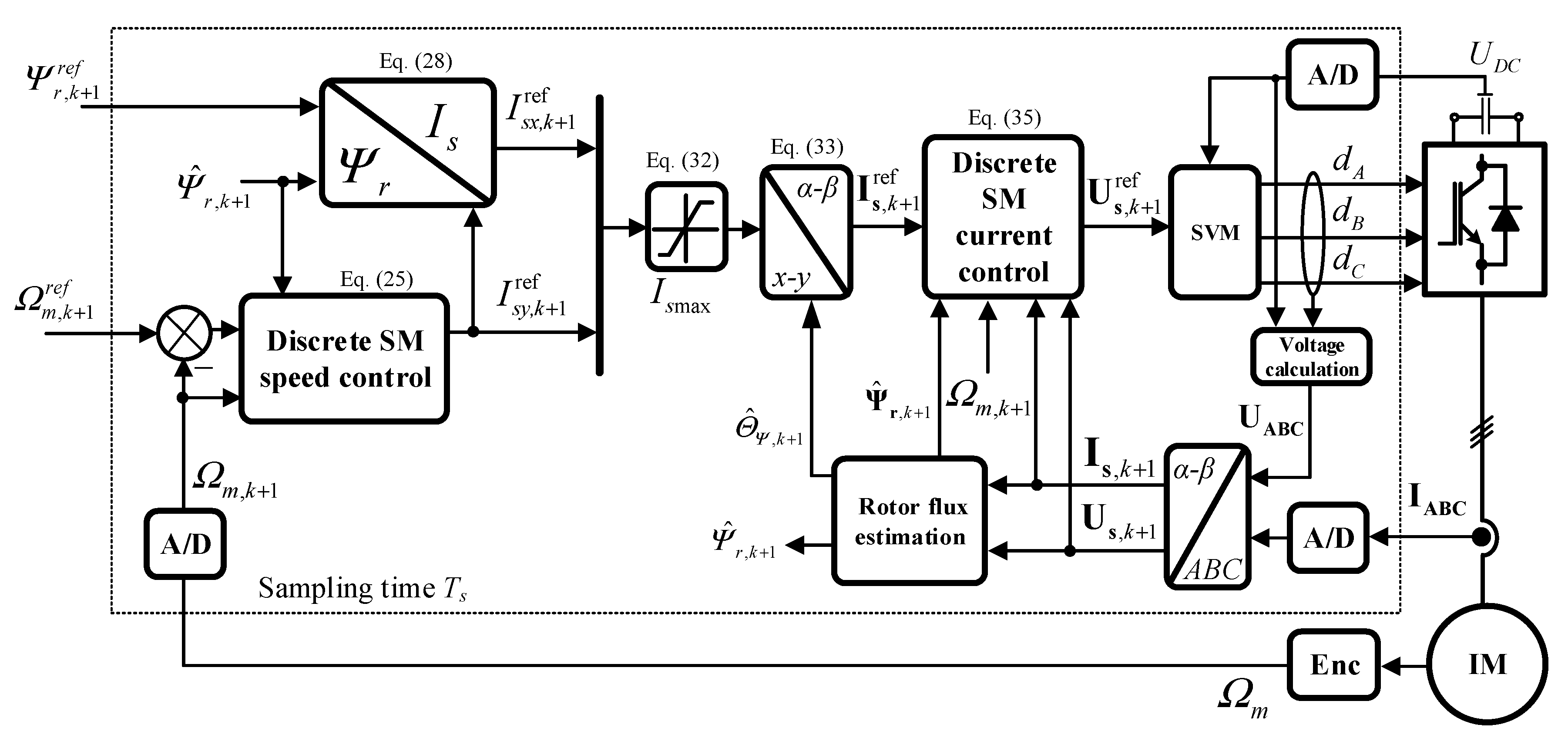
3.5. Overall Control Structure

The block diagram of the control structure is shown in Figure 1. The whole control algorithm is discretized with sampling time Ts. Due to the lower dynamics of the IM speed, the sampling time of the speed control algorithm could be decreased comparing to the current and flux control, however, it was not an assumption of this research.
The flux control algorithm (28) defines the first component of the reference stator current vector, based on reference flux amplitude value, estimated flux and the second reference stator current component. In this paper it is assumed that the rotor flux estimation is available and is ideal.
The proposed speed control algorithm (25) determines the second component of the reference stator current vector, based on the reference and real speeds and the estimated flux amplitude (necessary in order to calculate the switching function). Both stator current components are limited (33) and transformed into the stationary frame (33), using the estimated rotor flux vector angle.
Based on the reference signals, estimated flux, speed, current and voltage, the discrete SMC of the stator currents is applied (35). Its output is reference voltage signal, which becomes the input of the space vector modulation (SVM). Based on its output signals, i.e., duty cycles dA, dB, dC and the DC-bus voltage UDC, the motor voltage vector UABC is estimated. It is assumed that the stator currents IABC and the motor speed Ωm are measured by current transducers and incremental encoder (Enc), respectively.

4. Simulation Results

Wide simulation tests have been conducted to verify the operation of the proposed control structure. Various aspects of the operation have been checked: load torque impact, regulation time constants and sampling time influence. All tests are obtained using MATLAB/Simulink software, for the IM with rated data and parameters given in the Appendix A. The model of VSI and IM is sampled with 1e-6 s, using the Euler method. The control structure is sampled with 10 kHz, unless stated otherwise. The sampling and switching frequencies are the same.

4.1. Performance of the Control Structure

Performance of the proposed control structure is shown in Figure 2. It can be seen (Figure 2a) that the reference speed changes suddenly at 0.1 s and reaches 100% of its nominal value. The demanded dynamics of the rotor speed is marked as ω m dyn and indicated with blue color. The settling time of the speed control is equal to T = 3Tω = 0.25 s. The objective of the control structure is fulfilled, as the real speed of the drive follows the reference value with desired dynamics. At 0.5 s the drive is loaded with nominal torque. The speed reacts slightly and returns to its reference value very fast. Although many sliding-mode control algorithms have a tendency to induce a steady-state regulation error, usage of the proposed DSMC structure eliminates this phenomenon. It is connected with the form of the switching Function (20)—it uses x1, which is calculated with a numerical integration, using the forward Euler method (17).
Before the speed is controlled, the rotor flux amplitude is stabilized at its nominal level (Figure 2b) to ensure linear dependence between the torque and torque-producing current Isy. The flux is regulated with the settling time T = 3TΨ = 0.1 s, according to Equation (31). The torque of the motor is shown in Figure 2c. Its shape corresponds to the y-axis component of the stator current vector, shown in Figure 2e. Both components of the stator current vector are controlled precisely, as illustrated in Figure 2d,e, respectively.
The rotor speed phase trajectory is shown in Figure 2f. Three different stages of the regulation can be seen: the reaching phase, next the quasi-sliding phase and the load torque disturbance. After short reaching phase the speed trajectory remains in the vicinity of the sliding line, defined by Equation (20) and marked with a straight black line. Because of the discrete realization, the ideal sliding motion along the switching line is not possible. The trajectory tends to the origin of the coordinate system—the reference speed is equal to the real speed. The load torque appearance effects in a perturbation of the trajectory, since it leaves the close vicinity of the switching line for a short time. However, the speed returns to the origin again very fast. The switching function, as shown in Figure 2g remains near zero value—it reaches the highest values when the y-axis component of the stator current vector is close to its maximum value.
Speed time constant and final dynamics of the rotor speed can be easily modified according to the final drive application. This is shown in Figure 3. Performance of the control structure for four different time constants and four different load torque values are presented. The tests are made for half of the nominal speed. All of the trajectories start with the same point, defined by the difference between reference and real speed (x20 is about 78 rad/s) and zero value of the speed increase δΩm = 0. Then, they follow similar path, in order to reach the vicinity of the switching line finally. The lower the time constant, the lower the slope of the theoretical switching line and the faster the speed trajectory reaches its vicinity. Some small high-frequency oscillations (chattering) can be seen during the reaching phase. However, they vanish quickly. The second effect of the load torque is obvious—the accessible value of δΩm is limited by the difference between the motor and load torque (10).

4.2. Influence of the Sampling Time

The influence of the sampling frequency on the operation of the proposed DSMC is verified as well. In Figure 4, three different frequencies are analyzed: 500 Hz, 1000 Hz and 4000 Hz. After 0.7 s the nominal passive load torque appears, while a speed reversal takes place after about 1.0 s. It can be seen that the speed control is in all cases almost identical. The real speed follows the reference one with required dynamics. The only difference, visible in the transients is the influence of the load torque, the lower the sampling frequency, the influence is increased. The frequency of 500 Hz is in fact an extremely low sampling frequency for this power machines (see Appendix A). However, the behavior of the drive system is satisfactory. It must be stated that the control parameters must be modified for each applied sampling frequency, as shown below in Equation (26). The inequality of qTs < 1 can be rewritten to q < fs. Therefore, in the tests, the parameter is changed accordingly.

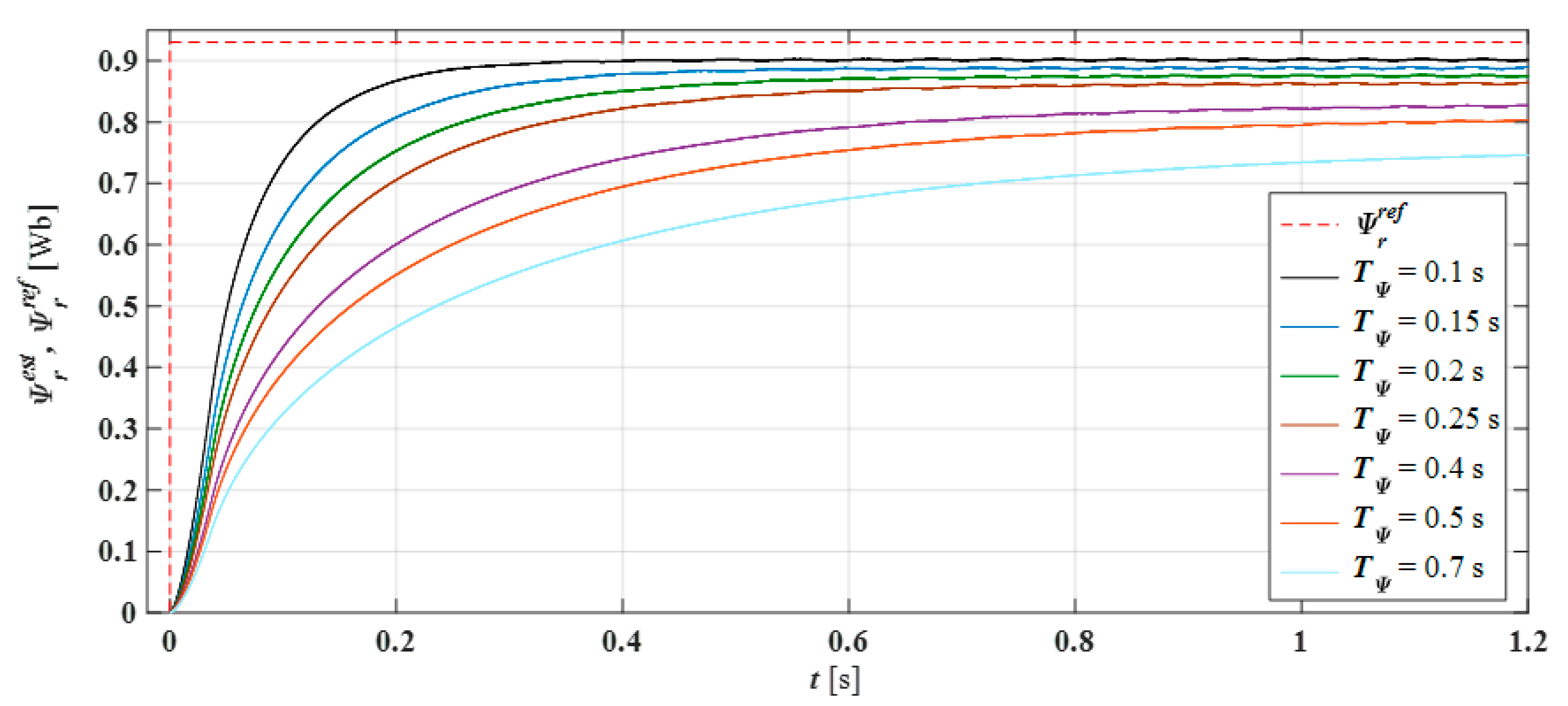
4.3. Time-Varying Switching Time

As was shown in Figure 3, speed trajectory during the reaching phase can be different depending on the disturbances, e.g., load torque. Therefore, in order to ensure the robustness during all regulation stages, including the reaching phase, the technique of moving switching line is applied (38). In order to verify the operation of the DSMC with time-varying switching line, a series of tests have been conducted (Figure 5 and Figure 6). The operation of the drive with different values of the load torque TL is presented in Figure 5. It can be seen that in the case of stationary switching line, the reaching phase is different in each shown case. Additionally, some oscillations arise during the reaching phase. On the contrary, when the moving switching line is applied, the speed phase trajectories all look the same. The drive is robust to different load torque values, as its behavior is the same in all analyzed cases.
Similarly, the operation of the drive is robust in the case of varying moment of inertia, when the time-varying switching line is implemented. It is shown in Figure 6b.

5. Experimental Tests

5.1. Experimental Setup

The block diagram and a photo from Figure 7 show the experimental setup used during the research. The key element of the setup was the rapid prototyping system based on National Instruments NI PXIe-1071. The setup was equipped with a field-programmable gate array (FPGA) and data acquisition (DAQ) cards. The FPGA card was responsible for generating PWM signals kA, kB, kC and counting impulses from the incremental encoder (En), to determine the speed of the drive Ωm. The DAQ card acquired analogue signals of stator phase currents IsA, IsB, IsC and the DC-bus voltage UDC of the voltage source inverter (VSI) that supplied the machine under consideration. These signals were measured with LEM transducers. The DAQ card transfers also required value of the load torque T L r e f to another industrial VSI supplying the load-generating machine. Industrial Permanent Magnet Synchronous Motor (PMSM) of 4.7 kW was used to ensure the load torque. It is equipped with a resolver (R) to determine the position of the shaft Θm.
Control of the TWERD VSI is made by a fiber-optics signals, therefore a card ensuring the transition between electrical and optical signals is applied—it can be seen in Figure 7b. This card is also responsible for generating the dead-time, equal to 2 μs in this case.

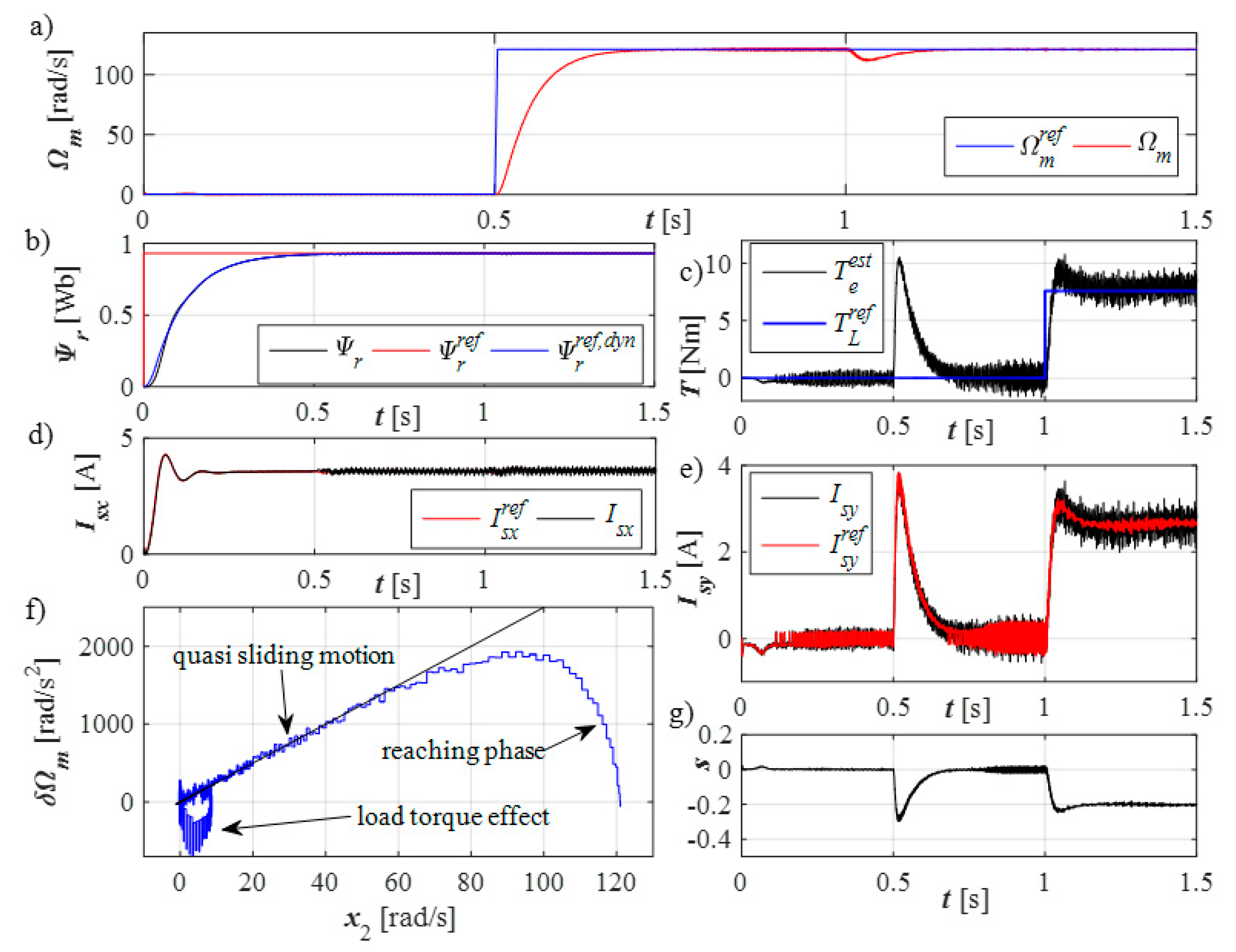
5.2. Experimental Test Results

As it was written in Section 3.2.2 the rotor flux control is based on discretized motor model and can be subjected to modelling errors and mismatched parameters. This phenomenon is presented in Figure 8. The reference rotor flux is equal to its nominal value, while the transients of estimated rotor flux amplitudes are shown for different values time constants TΨ. It can be shown that the steady-state error increases with increasing time constant. Due to this effect, in the following results the PI based flux control will be applied, while the reference signal is similar to first-order inertial dynamics.
Figure 9 presents the experimental test results being an equivalent to simulation study shown in Figure 2. First, performance of the control system without time-varying switching line is verified. It is shown that the speed of the motor follows precisely the reference speed (equal to 80% of its nominal value) with required dynamics. The speed settling time constant is small, equal to Ts = 0.15 s. The rotor flux amplitude is controlled in a similar exponential way, as can be seen in Figure 9b. As was mentioned before, the flux is controlled with a PI controller realized in a discrete-time domain. After about 1 second the load torque appears—it is presented in Figure 9c. The load torque is equal to 80% of its nominal value, and makes the speed drop slightly. This effect is bigger than the one obtained during the simulation tests. However, the speed returns to its reference value very fast and without any steady-state error. The components of the stator current vector (Figure 9d,e) are controlled effectively, with some acceptable level of noise. The level of the noise increases especially after the speed differs from zero. The phase portrait from Figure 9f is similar to the one from Figure 2f. After initial reaching phase the trajectory stays in the vicinity of the sliding line and goes towards zero (objective of the regulation). The appearance of the load torque disturbs the trajectory from the origin of the coordinate system. However, as said, it returns there very quickly. The switching function value has analogue shape as during simulation tests (Figure 2g), only its value is bigger.
The time-varying switching line is applied to verify its usefulness in ensuring the robustness of the drive from beginning of the motion (reaching phase) till reaching the origin of the coordinate system. Obtained results, for four different values of the load torque, are shown in Figure 10. They show the comparison of the performance of the speed control in the case of stationary (Figure 10a) and non-stationary switching lines (Figure 10b). The final position of the switching line is shown with black color in Figure 10b. Similarly to Figure 5, the application of the time-varying switching line causes that the speed phase trajectories are almost the same regardless the disturbance value. When the line is stationary the trajectories can vary significantly and the robustness of the operation is not guaranteed (Figure 10a).

6. Conclusions

This paper is focused on chattering-free discrete-time Sliding mode control of induction motor speed. Rotor flux amplitude as well as internal discrete control of the stator current components in the stationary reference frame is taken into account as well. The control structure ensures to take into account the constraints of both stator current and voltage as well ensures the rotor flux and speed are controlled to follow their reference values precisely, with the required dynamics.
Two different kinds of rotor flux amplitude control are considered. The one, based directly on the discretized mathematical model of the induction motor is proved to produce steady-state error, visible during the experimental tests. Therefore, in this paper, simple control with usage of the discretized PI controller is used.
A time-varying switching line concept is proposed to extend the DSMC, in order to ensure the robustness of the speed control structure over parametric and external disturbances, also during the reaching phase. It is shown that the phase trajectories are the same for different levels of load torque and values of moment of inertia. In this meaning the drive system is robust.
The influence of the sampling time on the control quality is verified as well. It is proved that the control quality deteriorates insignificantly if the sampling frequency decreases, however, it retains the required dynamics of the speed control.

Author Contributions

Conceptualization, T.O.-K. and G.T.; data curation, G.T.; formal analysis, T.O.-K. and G.T.; investigation, G.T.; methodology, T.O.-K. and G.T.; project administration, T.O.-K.; software, G.T.; supervision, T.O.-K.; visualization, G.T.; writing—original draft, T.O.-K. and G.T.; writing—review and editing, T.O.-K. All authors have read and agreed to the published version of the manuscript.

Funding

This research was financed by the National Science Center (Poland) under the project number 2015/17/B/ST7/03846 and partly by statutory funds of the Faculty of Electrical Engineering, Wroclaw University of Science and Technology.

Conflicts of Interest

The authors declare no conflicts of interest.

Appendix A

The parameters and nominal data of the motor are shown in Table A1.
Table A1. Induction Motor Parameters.
ParameterValue [Ph. U.]
Nominal powerPN = 1.5 [kW]
Nominal torqueTN = 10.16 [Nm]
Nominal voltageUN = 400 [V]
Nominal currentIN = 3.4 [A]
Nominal speednN = 1410 [rpm]
Main inductanceLm = 424.6 [mH]
Stator/rotor leakage inductanceL = L = 17.3 [mH]
Stator resistanceRs = 5.307 [Ω]
Rotor resistanceRr = 4.843 [Ω]
Rotor fluxΨr = 0.93 [Wb]
Nominal stator frequencyfsN = 50 [Hz]
Pair of polespb = 2
Moment of inertiaJN = 0.0117 [kg m2]

References

  1. Yu, X.; Kaynak, O. Sliding-Mode Control with Soft Computing: A Survey. IEEE Trans. Ind. Electron. 2009, 56, 3275–3285. [Google Scholar] [CrossRef]
  2. Utkin, V.I. Sliding mode control design principles and applications to electric drives. IEEE Trans. Ind. Electron. 1993, 40, 23–36. [Google Scholar] [CrossRef] [Green Version]
  3. Lascu, C.; Trzynadlowski, A.M. Combining the principles of sliding mode, direct torque control, and space-vector modulation in a high-performance sensorless AC drive. IEEE Trans. Ind. Appl. 2004, 40, 170–177. [Google Scholar] [CrossRef]
  4. Sabanovic, A. Variable Structure Systems with Sliding Modes in Motion Control—A Survey. IEEE Trans. Ind. Inform. 2011, 7, 212–223. [Google Scholar] [CrossRef]
  5. Panchade, V.M.; Chile, R.H.; Patre, B.M. A survey on sliding mode control strategies for induction motors. Annu. Rev. Control 2013, 37, 289–307. [Google Scholar] [CrossRef]
  6. Utkin, V.; Lee, H. Chattering problem in sliding mode control systems. In Proceedings of the International Workshop on Variable Structure Systems, Alghero, Italy, 5–7 June 2006; pp. 346–350. [Google Scholar]
  7. Castillo-Toledo, B.; Di Gennaro, S.; Loukianov, A.G.; Rivera, J. Discrete time sliding mode control with application to induction motors. Automatica 2008, 44, 3036–3045. [Google Scholar] [CrossRef]
  8. Castillo-Toledo, B.; Di Gennaro, S.; Galicia, M.I.; Loukianov, A.G.; Rivera, J. Indirect discrete-time sliding mode torque control of induction motors. In Proceedings of the XIX International Conference on Electrical Machines (ICEM), Rome, Italy, 6–8 September 2010. [Google Scholar]
  9. Quintero-Manriquez, E.; Sanchez, E.N.; Felix, R.A. Induction Motor Torque Control via Discrete-Time Sliding Mode. In Proceedings of the 16 International Joint Conference on Neural Networks, (IJCNN), Rio Grande, Puerto Rico, 31 July–4 August 2016; pp. 2756–2761. [Google Scholar]
  10. Tarchala, G. Discrete Sliding Mode Control of Induction Motor Torque and Stator Current Components. In Proceedings of the 18th IEEE International Power Electronics and Motion Control Conference (PEMC), Budapest, Hungary, 26–30 August 2018; pp. 675–680. [Google Scholar]
  11. Chern, T.L.; Liu, C.S.; Jong, C.F.; Yan, G.M. Discrete integral variable structure model following control for induction motor drivers. IEE Proc.-Electr. Power Appl. 1996, 143, 467–474. [Google Scholar] [CrossRef]
  12. Veselic, B.; Perunicic-Drazenovic, B.; Milosavljevic, C. High-Performance Position Control of Induction Motor Using Discrete-Time Sliding-Mode Control. IEEE Trans. Ind. Electron. 2008, 55, 3809–3817. [Google Scholar] [CrossRef]
  13. Veselic, B.; Perunicic-Drazenovic, B.; Milosavljevic, C.B. Improved Discrete-Time Sliding-Mode Position Control Using Euler Velocity Estimation. IEEE Trans. Ind. Electron. 2010, 57, 3840–3847. [Google Scholar] [CrossRef]
  14. Sarpturk, S.Z.; Istefanopulos, Y.; Kaynak, O. On the stability of discrete-time sliding mode control systems. IEEE Trans. Autom. Control 1987, 32, 930–932. [Google Scholar] [CrossRef]
  15. Furuta, K. Sliding mode control of a discrete system. Syst. Control Lett. 1990, 14, 145–152. [Google Scholar] [CrossRef]
  16. Sira-Ramirez, H. Non-linear discrete variable structure systems in quasi-sliding mode. Int. J. Control 1991, 54, 1171–1187. [Google Scholar] [CrossRef]
  17. Golo, G.; Milosavljević, Č. Robust discrete-time chattering free sliding mode control. Syst. Control Lett. 2000, 41, 19–28. [Google Scholar] [CrossRef]
  18. Choi, S.B.; Park, D.W.; Jayasuriya, S. A time-varying sliding surface for fast and robust tracking control of second-order uncertain systems. Automatica 1994, 30, 899–904. [Google Scholar] [CrossRef]
  19. Bartoszewicz, A. A time-varying sliding surface for fast and robust tracking control of second-order uncertain systems—A comment. Automatica 1995, 31, 893–1895. [Google Scholar] [CrossRef]
  20. Corradini, M.L.; Orlando, G. Linear unstable plants with saturating actuators: Robust stabilization by a time varying sliding surface. Automatica 2007, 43, 88–94. [Google Scholar] [CrossRef]
  21. Bartoszewicz, A.; Nowacka, A. Optimal design of the shifted switching planes for VSC of a third-order system. Trans. Inst. Meas. Control 2006, 28, 335–352. [Google Scholar] [CrossRef]
  22. Lesniewski, P. Sliding mode control with time-varying sliding hyperplanes: A survey. In Proceedings of the 18th International Carpathian Control Conference (ICCC), Sinaia, Romania, 28–31 May 2017; pp. 81–86. [Google Scholar]
  23. Betin, F.; Capolino, G.A. Sliding mode control for an induction machine submitted to large variations of mechanical configuration. Int. J. Adapt. Contr. Sign. Proc. 2007, 21, 745–763. [Google Scholar] [CrossRef]
  24. Chen, Z.M.; Zhang, J.G.; Zeng, J.C. A new method of sliding mode control and application to AC servo system. In Proceedings of the 5th International Conference Electrical Machines and Systems (ICEMS), Shenyang, China, 18–20 August 2001; pp. 759–762. [Google Scholar]
  25. Pang, H.-P.; Liu, C.-J.; Zhang, W. Sliding mode fuzzy control with application to electrical servo drive. In Proceedings of the 6th International Conference Intelligent Systems Design and Applications (ISDA), Jinan, China, 16–18 October 2006; pp. 320–325. [Google Scholar]
  26. Tarchala, G. Sliding mode speed control of an induction motor drive using time-varying switching line. Power Electron. Drives 2017, 2, 1310–1315. [Google Scholar] [CrossRef]
  27. Bartoszewicz, A. Discrete-time quasi-sliding-mode control strategies. IEEE Trans. Ind. Electron. 1998, 45, 633–637. [Google Scholar] [CrossRef]
  28. Hu, Q.; Du, C.; Xie, L.; Wang, Y. Discrete-time sliding mode control with time-varying surface for hard disk drives. IEEE Trans. Control Syst. Technol. 2008, 17, 175–183. [Google Scholar] [CrossRef]
  29. Kanai, Y.; Mori, Y. Discrete time sliding mode control with time varying switching hyper plane. In Proceedings of the 2008 SICE Annual Conference, Tokyo, Japan, 20–22 August 2008; pp. 2349–2352. [Google Scholar]
  30. Komurcugil, H. Rotating-sliding-line-based sliding-mode control for single-phase UPS inverters. IEEE Trans. Ind. Electron. 2011, 59, 3719–3726. [Google Scholar] [CrossRef]
  31. Zhang, J.; Zhang, Y.; Chen, Z.; Zhao, Z. A control scheme based on discrete time-varying sliding surface for position control systems. In Proceedings of the 5th Congress on Intelligent Control and Automation (WCICA), Hangzhou, China, 15–19 June 2004; pp. 1175–1178. [Google Scholar]
  32. Bayindir, M.I.; Can, H.; Akpolat, Z.H.; Ozdemir, M.; Akin, E. Robust quasi-time-optimal discrete-time sliding mode control of a servomechanism. Electr. Power Compon. Syst. 2007, 35, 885–905. [Google Scholar] [CrossRef]
  33. Sharma, N.K.; Roy, S.; Janardhanan, S. New design methodology for adaptive switching gain based discrete-time sliding mode control. Int. J. Control 2019. [Google Scholar] [CrossRef] [Green Version]
  34. Sharma, N.K.; Roy, S.; Janardhanan, S.; Kar, I.N. Adaptive Discrete-Time Higher Order Sliding Mode. IEEE Trans. Circuits Syst. II Express Br. 2019, 66, 612–616. [Google Scholar] [CrossRef]
  35. Kazmierkowski, M.; Krishnan, R.; Blaabjerg, F. Control in Power Electronics—Selected Problems; Academic Press—An imprint of Elsevier Science: Cambridge, MA, USA, 2002; p. 250. [Google Scholar]
  36. Tarchala, G. Influence of the stator current approximation form on the discrete sliding mode torque control for induction motor drive. In Proceedings of the 9th Joint Slovakian-Croatian International Conference on Electrical Drives & Power Electronics (EDPE), Novy Smokovec, Slovakia, 24–26 September 2019; pp. 66–73. [Google Scholar]
Figure 1. Block diagram of the proposed discrete-time sliding mode control (DSMC) structure.
Electronics 09 00185 g001
Figure 2. Performance of the proposed DSMC control structure: (a) real and reference speeds, (b) real and reference amplitude of the rotor flux, (c) electromagnetic and load torques, (d) reference, real and maximum x-axis component of stator current, (e) reference, real and maximum y-axis component of stator current, (f) speed phase trajectory, (g) switching function. Simulation study.
Electronics 09 00185 g002
Figure 3. Phase trajectories of the motor speed for different time constants and load torque values: (a) no load, (b) 10% of nominal torque, (c) 50% of nominal torque, (d) 100% of nominal torque. Simulation study.
Electronics 09 00185 g003
Figure 4. Performance of the proposed DSMC structure under reference speed changes (reverse operation) for different sampling frequencies: (a,b) sampling frequency 500 Hz (q = 100), (c,d) sampling frequency 1000 Hz (q = 250), (e,f) sampling frequency 4000 Hz (q = 750); reference and real speeds (left column); reference and real torque-producing current (right column). Simulation study.
Electronics 09 00185 g004
Figure 5. Influence of the load torque changes on the speed phase trajectory in the case of: (a) stationary, (b) time-varying switching line. Simulation study.
Electronics 09 00185 g005
Figure 6. Influence of the moment of inertia changes on the speed phase trajectories in the case of: (a) stationary, (b) time-varying switching line. Simulation study.
Electronics 09 00185 g006
Figure 7. Experimental setup: (a) block diagram, (b) photo.
Electronics 09 00185 g007
Figure 8. Influence of the rotor flux time constant on the operation of the model-based rotor flux control. Experimental study.
Electronics 09 00185 g008
Figure 9. Performance of the proposed DSMC control structure: (a) real and reference speeds, (b) real and reference amplitude of the rotor flux, (c) electromagnetic and load torques, (d) reference, real and maximum x-axis component of stator current, (e) reference, real and maximum y-axis component of stator current, (f) speed phase trajectory, (g) switching function. Experimental study.
Electronics 09 00185 g009
Figure 10. Influence of the load torque changes on the speed phase trajectory in the case of: (a) stationary, (b) time-varying switching line. Experimental study.
Electronics 09 00185 g010

