Online Learned Siamese Network with Auto-Encoding Constraints for Robust Multi-Object Tracking

Abstract

Multi-object tracking aims to estimate the complete trajectories of objects in a scene. Distinguishing among objects efficiently and correctly in complex environments is a challenging problem. In this paper, a Siamese network with an auto-encoding constraint is proposed to extract discriminative features from detection responses in a tracking-by-detection framework. Different from recent deep learning methods, the simple two layers stacked auto-encoder structure enables the Siamese network to operate efficiently only with small-scale online sample data. The auto-encoding constraint reduces the possibility of overfitting during small-scale sample training. Then, the proposed Siamese network is improved to extract the previous-appearance-next vector from tracklet for better association. The new feature integrates the appearance, previous, and next stage motions of an element in a tracklet. With the new features, an online incremental learned tracking framework is established. It contains reliable tracklet generation, data association to generate complete object trajectories, and tracklet growth to deal with missing detections and to enhance the new feature for tracklet. Benefiting from discriminative features, the final trajectories of objects can be achieved by an efficient iterative greedy algorithm. Feature experiments show that the proposed Siamese network has advantages in terms of both discrimination and correctness. The system experiments show the improved tracking performance of the proposed method.

1. Introduction

As a key technology in computer vision, multi-object tracking (MOT) has received growing attentions from researchers all over the world. In recent years, with the improvements in object detecting techniques [1,2,3], tracking-by-detection (TBD) has become one of the most successful strategies. It applies an object detector to produce detection responses in each frame, which are then used to generate complete trajectories. The data association process mainly depends on object features including appearance, motion, and other factors. It is often solved by Hungarian algorithms [4,5], network flows [6,7,8], minimum energy models [9,10], conditional random field approaches [11,12], hyper-graph model [13], deep learning methods [14,15,16,17], and so on.

Object feature expression is the basis of data association. Handcrafted features, such as the histogram of oriented gradient (HOG) [18], local binary patterns (LBP) [19], and the histogram of color (HOC) are widely used in computer vision researches [8,11,13,20]. These features were originally designed to distinguish objects from various backgrounds. Although a combination of different handcrafted features [11,13] is often used to improve discrimination, it is still not robust enough. Meanwhile, detection responses given by object detectors are not always accurate and sometimes even false due to complex backgrounds, poor image quality, complicated movements, or occlusions of objects. Thus, how to better distinguish targets by online detection responses, how to deal with noise due to detection inaccuracy, and how to combine various cues of a target to enhance discrimination remain key issues that limit tracking performance.

With the developments of deep learning in image classification, segmentation, and other applications, researchers used deep architectures to learn discriminative features for multi-object tracking, and they achieved good results. In [12,15,17,21,22,23], deep Siamese networks were adopted instead of traditional handcrafted methods [11,13]. A contrastive loss function was used with the aim of decreasing the feature distances for the same object pairs while increasing distances for the different pairs. Due to the shortage of online samples, training of such deep neural network mainly depends on offline learning. Although online fine-tuning measures are often adopted, the online data are too limited to run a deep network effectively.

In this paper, a Siamese network with an auto-encoding constraint (SNAC) is proposed, which is able to work well with a small-sized sample set. Different from previous deep Siamese networks, the SNAC has a simple structure with two fully-connected layers, an auto-encoder layer, and a code-mix layer. The simple network can be easily learned by online limited samples to extract discriminative features to distinguish objects on the scene. Inspired by stacked auto-encoder methods [24,25], the output of the encoder layer tries to represent the input detection response as accurately as possible. This is done by adding a constraint term to the loss function, called the auto-encoding constraint, which effectively prevents the network from overfitting while training with limited samples. To deal with inaccurate detection responses (red bounding box in Figure 1a), Gaussian distribution training samples are generated around detection responses to suppress noises. For each detection response, one SNAC is trained to distinguish it from others in adjacent frames. Meanwhile, in order to enhance robustness, following [22], the HOC is used as the input instead of raw pixels. With the discriminative detection features extracted by SNACs, reliable tracklets are generated.

To better distinguish tracklets, SNAC is improved to extract a composite previous-appearance-next (PAN) feature for each tracklet, which combines previous and next step motions with the appearance of the tracklet element. Following [11,26], elements in the same tracklet can be treated as positive samples, and the negative samples are obtained from time overlapped tracklets. The distribution is proposed to express motion that can suppress motion noises, and this is also compatible with the appearance for joint learning of the PAN feature.

In order to solve the MOT problem by the proposed SNAC, an online incremental learned tracking framework is established. First, one SNAC is trained for each detection response online, and reliable tracklets are generated mainly by the extracted features. Then, the PAN features are learned from tracklets by improved SNACs. To improve the training efficiency, SNACs are trained by incremental learning. During tracklet generation, the parameters of SNAC for detection in the new frame are inherited from the predecessor tracklet element, and the training samples are updated frame by frame. To extract PAN, the parameters are initialized by the SNAC of the related detection response. A tracklet growing process is used to deal with missing and partial detections (Figure 1b,c) before tracklet association. With the discriminative PAN feature, complete trajectories are solved efficiently by an iterative greedy algorithm. The main contributions of this paper are summarized as follows:

(1)

A simple structure Siamese network with an auto-encoding constraint is proposed to extract discriminative features efficiently for objects on the scene. An auto-encoding constraint is added to prevent overfitting when training data are limited.

(2)

A composite feature of tracklet, PAN, is defined, which combines appearance and motion through joint learning. To describe the sequential features of tracklets better, data association based on PAN is more reliable.

(3)

A tracking framework is established that includes reliable tracklet generation by incremental learning with SNAC for the detection response, tracklet growth to enhance PAN performance and deal with missing detections, and tracklet association with PAN to generate complete trajectories.

2. Related Works

Tracking by detection (TBD) has been one of the most promising methods developed to solve the multi-object tracking (MOT) problem in recent years. It generates object trajectories based on detection responses given by pre-designed detectors. For reliable data association, most recent researches were based on tracklets. In [26], the dual-threshold method was proposed to generate reliable tracklets and utilize them to get the final trajectories hierarchically. In [27], a prototype of a three frames triplet, which is a type of three members tracklet, was designed to extract high-level features. The Hungarian algorithm was also used to generate reliable tracklets in [12,15]. On the basis of tracklets, [11] built an online learning conditional random field (CRF) model focused on distinguishing the difficult pairs of objects. In [13], a hyper-graph model was developed to explore more complex relations among objects. The latest MOT methods [12,21] also focused on using tracklets. In these studies, tracklet building and feature expression are important to achieve reliable data association. In this section, MOT object feature extraction methods are mainly introduced.

From handcrafted methods to deep learning techniques, many studies have achieved significant improvements in extracting appropriate object features for MOT. In [11,13], a combination of multiple handcrafted features was proposed to distinguish objects by appearance. Their sample collection schemes were used in many following studies. The developments of deep learning have introduced new ideas for feature description in tracking areas. In [24,28,29,30], deep neural networks were adopted for single object tracking (SOT), and achieved significant improvements. In SOT problems, features of objects were used to distinguish them from the background. Different from SOT, MOT mainly distinguishes objects from each other. Due to this difference, the deep learning scheme of SOT cannot provide good results for MOT problems.

The deep learning methods for MOT can be summarized into two categories. The first builds a deep learning based tracking model to form the whole MOT system. Milan et al. [31] proposed a tracking model based on recurrent neural networks (RNN). The proposed RNN model described the whole tracking system including motion prediction, updating, object state judgment, and data association. It was trained online in an end-to-end manner to track various objects. Schulter et al. [14] proposed a deep network flow model for MOT, which instead of empirically hand-crafting costs, learned the parameterized costs of the network flow model by end-to-end training. This dynamic parameter setting method improved the robustness and accuracy of tracking. Zhou et al. [12] proposed a deep continuous conditional random field (DCCRF) model for solving online MOT problems. The unary term was used to provide a deep discriminative appearance feature for tracklet association, and a pairwise term was used to deal with inter-object relations. In [16], a deep neural network consisting of an encoder and a decoder was proposed. In their method, an encoder was a fully-connected network and a decoder was a bidirectional long short-term memory (LSTM). This network was able to learn the association matrix to solve MOT.

The second group uses a deep neural network to extract discriminative feature for each object. Unlike the previous kind, this method deals with the object feature extraction problem directly, and many researchers have followed this idea. Sadehgian et al. [32] proposed an RNN model jointly used the appearance, motion, and interactions of an object to encode a discriminative long-term temporal relationship using these cues. Their discriminative appearance features were extracted by a deep CNN. Son et al. [33] designed a quadruplet CNN (QCNN) network to learn the affinities among objects based on appearance and motion. The proposed quadruplet loss function guided the network to learn a temporally-smooth appearance model with motion-aware constraints. Features extracted from the QCNN included time continuity, which enhanced the discrimination. In addition, Siamese networks, first defined and used for signature verification, played an important role and have achieved good results in face identification [34], people re-identification [35], and many computer vision applications. Siamese networks are more suitable for distinguishing objects due to their symmetrical structures. Wang et al. [15] applied a Siamese CNN (SCNN) to construct an appearance affinity model for tracklets. They embedded a temporally-constrained multi-task mechanism in their training process. Leal-Taixé et al. [22] used an SCNN to estimate the likelihood of two objects using a multi-modal inputs including image and optical flow. Following [22], Yoon et al. [23] proposed the historical appearance matching method and trained a Siamese network by a two-step process to deal with noisy detections. In [17], a speeding method was proposed to remove redundant appearance matchings of SCNN for real-time tracking. In the DCCRF model [12], SCNN was also used to extract discriminative features. Based on SCNN, Bae et al. [21] proposed a confidence-based data association method for MOT. They utilized the SCNN to learn a discriminative appearance model from offline training datasets.

3. Online Learned Siamese Network with Auto-Encoding Constraint

In this section, a new Siamese network with an auto-encoding constraint (SNAC) is proposed. It is better at distinguishing objects in MOT. Benefiting from the simple structure of two fully-connected layers, an auto-encoder layer and a code-mix layer, the SNAC can be learned effectively. Meanwhile, with an auto-encoding constraint in the loss function, SNAC can prevent overfitting while training with limited online samples. In order to suppress detection noises, Gaussian distribution samples were generated around detection responses to make up the training set and HOC was used as the input instead of raw pixels. Then, an incremental learning algorithm was proposed to train the SNAC to generate reliable tracklets. Mathematical notations are listed in

Table 1. Notations.

Symbol	Definition
SNAC	Siamese network with an auto-encoding constraint
$d_i^t$	the $i^{\mathrm{th}}$ detection response in frame t
$D_t$	detection responses set in frame t
$\mathbb{D}=\{D_1,\dots ,D_t\}$	sequence of $D_i$ for $i=1,2,\dots ,t$
$T_k^t$	the $k^{\mathrm{th}}$ tracklet up to frame t
${\mathbb{T}}^t=\{T^1,\dots ,T^t\}$	set of all tracklets up to frame t
${\mathbf{F}}_t^k$	feature vector of SNAC for $T_k^t$
$\left\{d\right\}$	a set consisting of an element d
$D_t-\left\{d\right\}$	the set $D_t$ with d deleted
$\mathsf{\Psi }(.)$	the sample set
${\mathsf{\Lambda }}_a(T,d)$	appearance similarity between T and d
$\mathsf{\Lambda }(T,d)$	overall affinity between T and d

.

3.1. The Structure of SNAC

The two-layer structure of SNAC is shown in Figure 2a. Bounding boxes of detection responses were first resized to 48 × 32 as the inputs of the Siamese network. The two sub-networks (dashed boxes in Figure 2a) were identical in structure and share parameters including weights and biases. A contrastive loss function was employed to learn the Siamese network.

As shown in Figure 2b, each sub-network consisted of an auto-encoder layer and a code-mix layer. The first layer contained three parallel auto-encoders corresponding to the red, green, and blue channels of the input RGB image, respectively. Similar to [22], the inputs were R, G, and B histograms, not pixel values, and they were denoted as 256 dimensions vectors: $\mathbf{x}0$, $\mathbf{x}1$, and $\mathbf{x}2$. Because of limited samples, training based on pixel values may lead to overfitting. Meanwhile, the histogram can also suppress the detection noises. Each auto-encoder contained a forward encoder, a backward decoder, and an auto-encoding error evaluator. The encoder and decoder were fully-connected networks. The output of the encoder was a vector with 100 dimensions, and the output of the decoder was a reproduction of the corresponding input. The code-mix layer was fully connecting and combined three code vectors of the first layer to produce a feature vector with 100 dimensions as the final output. Mathematically, the sub-network can be written as:

$$\left\{\begin{array}{c}{\mathbf{y}}_m^k=\sigma ({\mathbf{W}}_E^k{\mathbf{x}}_m^k+{\mathbf{b}}_E^k),m=p,q,k=0,1,2\hfill \\ {\widehat{\mathbf{x}}}_m^k=\sigma ({\mathbf{W}}_D^k{\mathbf{y}}_m^k+{\mathbf{b}}_D^k),m=p,q,k=0,1,2\hfill \\ {\mathbf{z}}_m=\sigma ({\mathbf{W}}_M({\mathbf{y}}_m^0,{\mathbf{y}}_m^1,{\mathbf{y}}_m^2)+{\mathbf{b}}_M),m=p,q\hfill \end{array}\right.$$

(1)

where subscript m indexes the upper p or lower q sub-network, the upper-script k indexes the channel, $\mathbf{y}$ is the code vector from an encoder, $\widehat{\mathbf{x}}$ is the reproduction of $\mathbf{y}$ by the decoder, and $\mathbf{z}$ is the final feature vector. $\mathbf{W}$, $\mathbf{b}$, and $\sigma$ are the weights, biases, and activation functions of the neural networks, with the subscripts E, D, and M indicating the encoder, decoder, and code-mix layer.

3.2. Loss Function and Auto-Encoding Constraint

To learn a Siamese network, a contrastive loss function was formulated based on similarity or difference measurements between input pair. The objective was to train the network to sufficiently reduce differences between pairs of the same inputs and to increase feature distances of different ones. The distance of input training pair is denoted as:

$$\begin{array}{c}\hfill D({\mathbf{x}}_p,{\mathbf{x}}_q)=\left|\right|{\mathbf{x}}_p-{\mathbf{x}}_q{\left|\right|}_2^2\end{array}$$

(2)

where ${\mathbf{x}}_p$ and ${\mathbf{x}}_q$ are feature vectors from the two sub-networks in SNAC. Instead of using the Euclidean distance here, other measures, like Mahalanobis and Bhattacharyya distances, can be used.

Given a group of training samples, the loss function of SNAC to be minimized consists of three terms, L1, L2, and L3, as follows:

$$\begin{array}{cc}\hfill L& =\alpha L1+\beta L2+\gamma L3\hfill \\ & =\alpha \sum _{p,q}max(0,\delta -l_{pq}[1-||{\mathbf{z}}_p-{\mathbf{z}}_q{\left|\right|}_2^2\left]\right)\hfill \\ & +\beta \sum _{k=0,1,2}\left|\right|{\mathbf{x}}_j^k-{\widehat{\mathbf{x}}}_j^k{\left|\right|}_2^2\hfill \\ & +\gamma (\sum _{k=0,1,2}\left|\right|{\mathbf{W}}_k{\left|\right|}_2^2+\left|\right|{\mathbf{b}}_k{\left|\right|}_2^2)\hfill \end{array}$$

(3)

where $\alpha$, $\beta$, and $\gamma$ are weight coefficients between zero and one. The first term, L1, is a margin-based loss of difference of sample pairs; $\delta$ is the decision margin, which satisfies ($0\le \delta \le 1$); $l_{pq}$ is the sample indicator; $l_{pq}=1$ denotes a positive pair; and $l_{pq}=0$ denotes a negative pair. The L3 term is the regularization constraint.

However, deep neural networks contain a large number of parameters and require huge sample sets for training. For the case of using limited online samples, parameters of a deep model will often be overfitting after training, and the network will not work. This method often pays more attentions to some local details of training samples and does not balance the general features. Subsequently, inspired by the stacked auto-encoder in [24,25], the L2 term was added, an auto-encoding constraint (AC) to the loss function in Equation (3), to prevent overfitting, even when training with limited online samples.

3.3. Denoising through the Collection of Training Samples

$D_t=\{d_i^t,i=1,2,\dots N_t\}$ is the detection set at frame t. Each detection response $d_i^t$ was associated with the SNAC$\left(d_i^t\right)$. Training samples were collected around $d_i^t$. The purpose of SNAC$\left(d_i^t\right)$ is to distinguish $d_i^t$ from other object detection responses in adjacent frames, not over a longer time period. The training samples of SNAC$\left(d_i^t\right)$ were collected online. Inspired by [11], $d_i^t$ is the only one positive sample, and the remaining detection responses at frame t constitute the negative sample set. Although SNAC$\left(d_i^t\right)$ can be trained by small-sized samples, an unbalanced sample set with only one positive sample cannot drive it. To solve this problem, more samples are needed, which means additional detection responses of $d_i^t$.

There is a fundamental issue whereby detection responses are not always perfect, and their bounding boxes are often inaccurate, as explained before in Figure 1a. When a noisy detection is used as a training sample, it will impair the parameters of SNAC. However, detection noise is inevitable, so this error can be suppressed through more $d_i^t$ with random noise. This noise processing is just enough to solve the positive sample shortage problem.

Detection noise was assumed to be modeled as additive noise as follows:

$$\begin{array}{c}\hfill {\mathbf{p}}_n=\mathbf{p}+{\mathbf{n}}_p,{\mathbf{s}}_n=\mathbf{s}+{\mathbf{n}}_s\end{array}$$

(4)

where $\mathbf{p}=(x,y)$ is the center position of the detection response, $\mathbf{s}=(w,h)$ is the size vector of width and height, and ${\mathbf{n}}_p$ and ${\mathbf{n}}_s$ are additive noises that refer to position and size, respectively. ${\mathbf{n}}_p$ and ${\mathbf{n}}_s$ are assumed to follow a Gaussian distribution, $G(0,{\sigma }_p)$ and $G(0,{\sigma }_s)$, where ${\sigma }_p$ and ${\sigma }_s$ are corresponding covariances obtained by prior analysis.

A group of random bounding boxes $\mathsf{\Psi }\left(\left\{d_i^t\right\}\right)$ was generated around $d_i^t$ according to Equation (4) with distributions of ${\mathbf{n}}_p$ and ${\mathbf{n}}_s$. In the same way, $\mathsf{\Psi }(D_t-\left\{d_i^t\right\})$ was obtained. $\mathsf{\Psi }\left(\left\{d_i^t\right\}\right)$ and $\mathsf{\Psi }(D_t-\left\{d_i^t\right\})$ are the positive and negative sample sets, respectively. Using these online collected samples, SNAC$\left(d_i^t\right)$ not only can extract discriminative features for $d_i^t$, but it also can suppress detection noises.

3.4. Iterative Tracklet Generation with SNAC by Incremental Learning

The above sections discussed the establishment and training of SNAC. Each detection response $d_i^t$ is associated with SNAC$\left(d_i^t\right)$, which extracts discriminative features to better distinguish $d_i^t$ from other detections belonging to $D_{t+1}$. Moreover, connecting these original independent networks not only increases the number of samples, but can also improve the training efficiency. On the one hand, SNAC$\left(d_i^t\right)$ can obtain more training samples from $d_j^{t-1}$ in the adjacent frame $t-1$ through a relationship. On the other hand, with this relationship, SNAC$\left(d_i^t\right)$ does not need random initialization parameters for training, but inherits them from SNAC$\left(d_j^{t-1}\right)$, which can reduce the training time to improve the efficiency. This relationship is the principle of tracklet linking, that is the two detection responses between adjacent frames belong to the same object. Incremental learning of SNACs through this inheritance relationship can effectively match adjacent frame detection responses. To generate reliable tracklets, an iterative algorithm with SNAC by incremental learning is proposed as shown in Algorithm 1.

Algorithm 1 Iterative tracklet building with SNAC by incremental learning.

Input:$\mathbb{D}=\{D_1,D_2,\dots ,D_t\}$, detection set of each frame

Output:${\mathbb{T}}^t=\left\{T_k^t\right\}$, tracklet setup to frame t   1: Initialization: $t=1$, ${\mathbb{T}}^1=\varnothing$   2: for each $d\in D_1$ do   3:     $T_k^1=d$   4:     Initialize ${\mathbf{F}}_k^1$ with random parameters   5:     Set $P=\mathsf{\Psi }\left(d\right)$, $N=\mathsf{\Psi }(D_1-d)$   6:     Train ${\mathbf{F}}_k^1$ with P and N   7: end for   8: while$t\ge 2$do   9:     for each $T_k^{t-1}\in {\mathbb{T}}^{t-1}$ and each $d\in D_t$ do 10:         Compute ${\mathsf{\Lambda }}_a(T_k^{t-1},d)$ as Equation (6) 11:         Compute $\mathsf{\Lambda }(T_k^{t-1},d)$ as Equation (5) 12:     end for 13:     For all $\mathsf{\Lambda }(T_k^{t-1},d)$ meeting the link requirement, select 14:     pairs of $T_k^{t-1}$ and d by the Hungarian algorithm. 15:     ${\mathbb{T}}^t=$ renewed ${\mathbb{T}}^{t-1}$ by linking the selected pairs. 16:     $D_t^R=D_t$ 17:     for each $T_k^t\in {\mathbb{T}}^t$ having a new detection added do 18:         $d=$ the new detection of $T_k^t$ 19:         Set $P=\mathsf{\Psi }\left(d\right)$, $N=\mathsf{\Psi }(D_t-d)$ 20:         ${\mathbf{F}}_k^t={\mathbf{F}}_k^{t-1}$ incrementally trained with P and N 21:         $D_t^R=D_t-d$ 22:     end for 23:     for each $d\in D_t^R$ do 24:         Add a new single member tracklet $T_k^t=d$, 25:         and set its ${\mathbf{F}}_k^t$ as above. 26:     end for 27: end while

At the first frame $t=1$, a new tracklet $T_i^1$ was established by a single member of $d_i^1$ in $D_1$, and the current total number of tracklets was $N_1$. To match the detection response belonging to the same object (or inexistence) in the next frame, a randomly initialized network, SNAC$\left(d_i^1\right)$, was associated with $d_i^1$. After SNAC$\left(d_i^1\right)$ training, the appearance similarity ${\mathsf{\Lambda }}_a(T_i^1,d_j^2)$ can be calculated by $T_i^1$, which is equal to $d_i^1$ and $d_j^2$. Together with the position similarity ${\mathsf{\Lambda }}_p(T_i^1,d_j^2)$ based on position and size, the total similarity $\mathsf{\Lambda }(T_i^1,d_j^2)$ can be calculated. When similarities of all detection responses in Frame 1 have been calculated, the Hungarian algorithm was used to determine if there was a $d_j^2$ that could be combined with $T_i^1$. If $d_i^1$ and $d_j^2$ belong to the same object, $d_j^2$ joins with $T_i^1$, and tracklet $T_i^1$ is updated to $T_i^2$. Otherwise, a new tracklet $T_{N_1+1}^2$ of $d_j^2$ is generated. Then, the processing went into Frame 2, and tracklets that contained the detection responses in Frame 2 needed to train. Taking $T_i^2$ as an example, its last element was $d_j^2$. If $d_i^1$ exists as a former element of $d_j^2$ in tracklet $T_i^2$, the initial parameters of SNAC$\left(T_i^2\right)$ equal to SNAC$\left(d_j^2\right)$ will be inherited from the trained SNAC$\left(d_i^1\right)$. In addition, the positive and negative training sets can be expanded through the samples of SNAC$\left(d_i^1\right)$. Training of SNAC$\left(T_i^2\right)$ can be done with fewer iterations in this incremental manner. If $T_i^2$ is a new added tracklet that only contains $d_j^2$, SNAC$\left(T_i^2\right)$ will be trained similarly to SNAC$\left(d_i^1\right)$. Finally, all reliable tracklets $\mathbb{T}$ will be produced frame-by-frame.

Now, the calculation of similarities between a tracklet and a detection response is explained. $\mathsf{\Lambda }(T_k^{t-1},d_j^t)$ is given as follows:

$$\begin{array}{c}\hfill \mathsf{\Lambda }(T_k^{t-1},d_j^t)={\mathsf{\Lambda }}_a(T_k^{t-1},d_j^t){\mathsf{\Lambda }}_o(T_k^{t-1},d_j^t).\end{array}$$

(5)

The appearance similarity was computed by the distance between feature vectors output by the SNAC$\left(T_k^{t-1}\right)$. It is given by:

$${\mathsf{\Lambda }}_a(T_k^{t-1},d_j^t)=g\{\parallel {\mathbf{F}}_k^{t-1}\left(\left(T_k^{t-1}\left(e\right)\right)\right)-{\mathbf{F}}_k^{t-1}\left(d_j^t\right){\parallel }_2^2\}$$

(6)

where $T_k^{t-1}\left(e\right)$ denotes the end element of tracklet $T_k^{t-1}$, ${\mathbf{F}}_k^{t-1}$ denotes the output feature vector of the SNAC for tracklet $T_k^{t-1}$, and g is a probability function on the squared distance of feature vectors. Because of the margin-based loss of SNAC, the definition of function g is as follows:

$$g\left(x\right)=\left\{\begin{array}{cc}1& x<1-\delta \\ 0& x>1+\delta \\ (1+\delta -x)/2\delta & otherwise\end{array}\right.$$

(7)

where $\delta$ is the decision margin given in the loss function of Equation (3).

Overlapping is widely used to describe the detection position relationship. It takes information about the coordinates and size into account. The overlapping ${\mathsf{\Lambda }}_o(T_k^{t-1},d_j^t)$ is given as:

$$\begin{array}{c}\hfill {\mathsf{\Lambda }}_o(T_k^{t-1},d_j^t)=\frac{A_{\cap }(T_k^{t-1}\left(e\right),d_j^t)}{min[A(T_k^{t-1}\left(e\right),A(d_j^t)]}\end{array}$$

(8)

where A is the area function on a detection response and $A_{\cap }$ is the area function on the intersection of two detection responses.

4. Multi-Object Tracking Framework

4.1. Overall Framework

Based on SNAC, a tracking framework following TBD was established to solve the MOT problem. A TBD scheme can be described as solving an MAP problem by:

$${\mathcal{T}}^{*}=\underset{\mathcal{T}}{argmaxP}\left(\mathcal{T}\right|\mathbb{D})$$

(9)

where $\mathbb{D}$ is the set of given detection responses and $\mathcal{T}$ is the set of trajectories. In the framework, tracklets were first generated. Because a tracklet is an ordered combination of detection responses, it is able to extract higher order features to better describe relations between objects. Then, the problem can be converted into a more reliable tracklet association as follows:

$${\mathcal{T}}^{*}=\underset{\mathcal{T}}{argmaxP}\left(\mathcal{T}\right|\mathbb{T})$$

(10)

where $\mathbb{T}$ is the set of all tracklets.

The whole framework is shown in Figure 3. First of all, the inputs were checked, and deformity detection responses were deleted, such as too large or small bounding boxes. SNAC was proposed to extract discriminative appearance features for detection responses. The online SNAC incremental learning method mentioned above was used to generate reliable tracklets. The next step was to generate tracking results through tracklet association. Similar to detection association based on the learning method, SNAC was improved to extract a new discriminative composite feature PAN for the tracklet instead of using traditional handcrafted methods. To enhance tracklet association, the tracklet growing module was embedded to make tracklets as extended as possible. With the discriminative PAN feature, tracklet association was converted to a linear programming problem that was solved by an efficient greedy iterative algorithm, and the final trajectories were achieved. For real-time tracking, the whole tracking process was carried out in sliding time windows.

4.2. Previous-Appearance-Next Feature of the Tracklet

A tracklet $T_m^{t2}=\{d_i^{t1},d_j^{t1+1},\dots d_k^{t2}\}$ is an ordered sequence of detection responses that represents a moving object with a short time from frame $t1$–$t2$. To describe $T_m^{t2}$, appearance and motion are indispensable. They are often assumed to be independent of each other in several studies [12,21,36]. Only by weighted summation can they express the similarity between two tracklets. To increase the flexibility and discrimination, a composite previous-appearance-next (PAN) feature was proposed. The new feature combined appearance and motion for the tracklet, and it was extracted jointly by an improved SNAC.

Taking $T_m^{t2}$ and $T_n^{t4}$ as examples, as shown in Figure 4b, $T_n^{t4}$ is from frame $t3$–$t4$ and $t2<t3$. To calculate the similarity between $T_m^{t2}$ and $T_n^{t4}$, it is better to use the tail part of $T_m^{t2}$ and the head part of $T_n^{t4}$ rather than using their whole information. $T_m^{t2}\left(e\right)$ is the last element of tracklet $T_m^{t2}$, and $T_n^{t4}\left(s\right)$ is the first element of $T_n^{t4}$. The PAN($T_m^{t2}\left(e\right)$) vector integrated the appearance, previous, and next stage motions of $T_m^{t2}\left(e\right)$ to express the tail part composite feature of tracklet $T_m^{t2}$. Correspondingly, the PAN($T_n^{t4}\left(s\right)$) vector was defined for the head part composite feature of $T_n^{t4}$. The next stage motion of tail $T_m^{t2}$ and the previous of head $T_n^{t4}$ were computed by estimation methods.

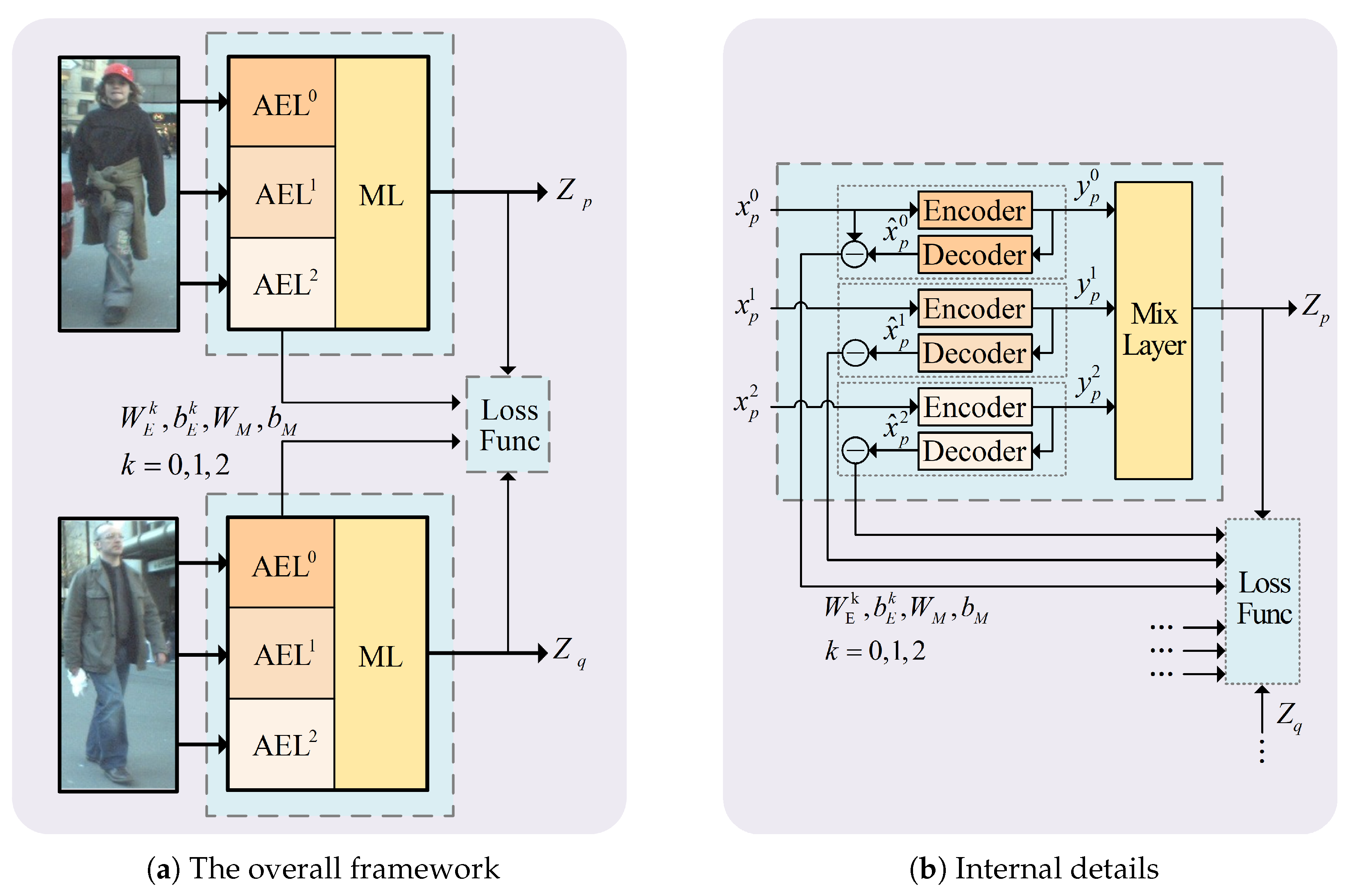
The SNAC for detection response was revised to extract PAN(.) vectors of tracklets. The new structure is shown in Figure 4a. The previous and next stage motions were used as additional inputs to the mix-layer. The first layer of the new SNAC was same as the old SNAC. ${\Delta }^p=(x^p,y^p)$ and ${\Delta }^n=(x^n,y^n)$ are the previous and next motion vectors of $T_m^{t2}\left(e\right)$, respectively. As shown in Figure 4b, ${\Delta }^p$ represents the $\mathit{x}$ and $\mathit{y}$ axes displacements of $T_m^{t2}$ from $t2-1$ to $t2$. For the next-stage motion vector, $T_m^{t2}(e+1)$, the estimation of $T_m^{t2}$ in frame $t2+1$ was computed first, and then, ${\Delta }^n$ of $T_m^{t2}\left(e\right)$ was calculated.

Since ${\Delta }^p$ and ${\Delta }^n$ are two-dimensional vectors that include displacements with x and y directions and the output of each auto-encoder in the first layer of SNAC is a 100-dimension feature vector, they are totally different in type and cannot work together simply. Meanwhile, the existence of detection noises makes the deterministic motion descriptions inaccurate. A distribution description method was proposed to represent the motion instead of specific values. Assuming following the Gaussian distribution, the $\mathit{x}$ axis displacement, $x^p$ of ${\Delta }^p$ for instance, is described by $G(x^p,{\sigma }_x)$, where ${\sigma }_x$ is set by pre-training. $G(y^p,{\sigma }_y)$ is for y displacement, as well. The distribution description was given by sample vectors of $G(x^p,{\sigma }_x)$ and $G(y^p,{\sigma }_y)$, and its length was taken to be equal to that of the appearance vector. For in MOT, the motion feature is as important as appearance. The distribution description for ${\Delta }^n$ can also be obtained. Then, they were merged with the three outputs of the first layer to form one mixed vector for the second-layer training.

Then, SNAC($T_m^{t2}\left(e\right)$) was trained to extract the tail PAN($T_m^{t2}\left(e\right)$) feature. Training samples of SNAC($T_m^{t2}\left(e\right)$) were also collected online. Similar to [11], elements in $T_m^{t2}$ are positive samples. Tracklets that overlap with $T_m^{t2}$ in time are positive samples. The parameters of the first layer were inherited from the corresponding detection SNAC. After training the SNAC($T_m^{t2}$), discriminative local composite features can be extracted to distinguish $T_m^{t2}$ from other subsequent tracklets.

As shown in Figure 4b, similarities between tracklet $T_m^{t2}$ and $T_n^{t4}$ were computed. After training, PAN$\left(T_m^{t2}\left(e\right)\right)$ and PAN$\left(T_n^{t4}(s+1)\right)$, as shown by the blue dashed circle areas in the figure, were extracted. Then, forward similarity was achieved as follows:

$$S_{m,n}^F=\left|\right|PAN\left(T_m^{t2}\left(e\right)\right)-PAN\left(T_n^{t4}(s+1)\right){\left|\right|}_2^2$$

(11)

To get a reliable similarity, the backward relationship was also computed, as shown in Equation (12).

$$S_{m,n}^B=\left|\right|PAN\left(T_m^{t2}(e-1)\right)-PAN\left(T_n^{t4}\left(s\right)\right){\left|\right|}_2^2$$

(12)

The final similarity was given by:

$${\mathsf{\Lambda }}_{PAN}(T_m,T_n)=g(min(S_{m,n}^F,S_{m,n}^B))$$

(13)

where g is the probability function for the distance of feature vectors, as defined in Equation (7).

4.3. Tracklet Growing

If the frame gap between $T_m^{t2}$ and $T_n^{t4}$ was small, variations in the appearance and motion from $T_m^{t2}$–$T_n^{t4}$ were not obvious, and the PAN could work well. Otherwise, the long-term frame gap brought a large variety of appearances, and motions may reduce the performance. PAN considers more local elements of the tracklet to enhance the performance. In order to make tracklet association more reliable, it is effective to reduce the time interval in the sliding windows as much as possible. Therefore, the tracklet growing process was used to extend the tracklet by estimated bounding boxes, which were missing from the detection. It contained forward and backward growth.

To forward the extended tracklet $T_m^{t2}$, the center position ${\mathbf{p}}_1^f\left(T_m^{t2}\right)=(\widehat{x},\widehat{y})$ in frame $t2+1$ was first estimated by quadratic fitting. Then, the optimal estimation bounding box was searched as follows:

$$\begin{array}{c}{d}^{*}=arg\underset{d\in C}{min}{∥\mathbf{H}\left(T_m^{t2}\left(e\right)\right)-\mathbf{H}\left(d\right)∥}_2^2\hfill \\ s.t.∥\mathbf{H}\left(T_m^{t2}\left(e\right)\right)-\mathbf{H}\left(d\right)∥\le {\epsilon }_1\hfill \end{array}$$

(14)

where C is the candidate bounding boxes set, center positions x and y are sampled according to the distribution of $G(0,{\sigma }_m)$, and the size is equal to $T_m^{t2}\left(e\right)$. $\mathbf{H}$ denotes the color histogram of detection $T_m^{t2}\left(e\right)$. The goal was to find the most similar estimation. If the optimal estimation $d_o^{t2+1}$ was found, a conflict process was also required to avoid false alarms. If the overlap between $d_o^{t2+1}$ and an existing $d_i^{t2+1}$ exceeded the threshold, the forward growth of $T_m^{t2}$ stopped. Otherwise, $T_m^{t2}$ was updated to $T_m^{t2+1}$ with $d_o^{t2+1}$ and the growing process continued to frame $t2+2$. The backward extension was similar to the forward process. For the isolated tracklets, random sampling was used to form the candidate estimations. After these missing detection compensation processes, tracklets were extended to improve the discrimination performance of PAN, and more reliable associations could be made.

4.4. Tracklet Association in Sliding Windows

Tracklet association was the last module in MOT to generate the final trajectories of objects. The main task was to link tracklets belonging to the same objects into a complete trajectory based on similarities among tracklets. Solutions such as min-cost networks, energy minimization, successive shortest paths, and the Hungary algorithm are widely used to generate tracking results. Global optimization is an ideal scheme because the previous judgments will be revised to achieve the overall optimal results. In cases where it is difficult to distinguish objects, this dynamic scheme can achieve better tracking performance than a greedy strategy. Similar to tracking by learning feature extraction method [15], network flows methods were no longer used to get the tracking result. The MAP problem shown in Equation (10) was directly mapped to a generalized linear assignment:

$$\begin{array}{c}\underset{L}{max}\sum _{i=1}^N\sum _{j=1}^N\mathsf{\Lambda }(T_i,T_j)L_{ij}\hfill \\ s.t.\sum _{i=1}^N{L}_{ij}\le 1;\sum _{j=1}^N{L}_{ij}\le 1\hfill \end{array}$$

(15)

To solve problem Equation (15), the similarity $\mathsf{\Lambda }(T_i,T_j)$ between tracklets was used; this is equal to linking probabilities mainly based on PAN features. $\mathsf{\Lambda }(T_i,T_j)$ was computed by Equation (13). However, PAN features cannot be extracted from tracklets with lengths of less than two elements. For this particular case, $\mathsf{\Lambda }(T_i,T_j)$ degenerated into the traditional weighted combination of appearance and motion. $L_{ij}$ is the association indicator, where 1 indicates connection and 0 means disconnection. The constraints guaranteed the uniqueness of association. As the better discriminative PAN, the similarity matrix $\mathsf{\Lambda }$ was normalized, and Equation (15) was solved by a greedy iterative algorithm.

5. Experiments

In this section, the performance of SNAC is first evaluated on detection responses and tracklets. Then, the proposed MOT system is tested on the MOT Challenge Benchmark [37].

5.1. Evaluation of SNAC

In the MOT system, the SNAC was proposed to extract discriminative features for detection responses and tracklets instead of handcrafted methods. Discrimination and accuracy were used as the main indicators to evaluate the performance of SNAC. Meanwhile, the effects of histogram inputting and the auto-encoding constraint were also evaluated. According to the order of the system framework, the performance of SNAC was first evaluated on detection responses and then tested the SNAC on tracklets. Since current public platforms do not provide annotation data for tracklets, how to make a fair comparison is a thorny issue. Therefore, the performance of SNAC was mainly compared with different constraints and handcrafted methods. In this experiment, the training processes of SNAC were carried out with graphics processing units (GPUs).

5.1.1. SNAC for Detection Responses

During tracklet generation, an SNAC$\left(d_i^t\right)$ was established for each detection response $d_i^t$ to implement the explicit frame-by-frame association. Through an online learning process, SNAC$\left(d_i^t\right)$ was able to extract features for $d_i^t$ and $D_{t+1}$. Then, the similarity between $d_i^t$ and each detection of $D_{t+1}$ could be obtained by the Euclidean distance. Statistical discrimination and variance of SNAC$\left(d_i^t\right)$ from these similarities can be calculated. Discrimination reflects the strength of the distinguishing ability, and variance represents the robustness. To generate the tracklet set in sliding temporal windows, each SNAC$\left(d_i^t\right)$ was trained by an incremental learning algorithm. Indicators of discrimination and variance were computed from the overall results. Another important indicator in evaluating the SNAC is the tracklet accuracy (TA). To compute TA, tracklets were treated as the final tracking results in a time window, so the metrics of MOT [38] could be used to evaluate the accuracy of tracklets. In this case, the core indicator MOTA was equal to the TA in Equation (15):

$$\begin{array}{c}\hfill TA=1-\frac{{\sum }_t(F{N}_t+F{P}_t+ID{s}_t)}{{\sum }_{t}G{T}_t}\end{array}$$

(16)

where t is the frame index in the current time window; FN, FP, and IDs are the number of false negatives, false positives, and mismatches, respectively; and GT is the number of ground truth tracklets annotated by us in this experiment.

Three subsequences of the 2DMOT2015 dataset were chosen to do this experiment. TUD-Crossing is a static camera scene, ETH-Jemoli and EHT-Linthescher are moving camera sequences. Three time windows are selected from each sequence to create a total of nine video segments for the experiment. GTs of the nine video segments are annotated.

As shown in

Table 2. Performance comparison of different features of detection responses. Red represents the best, and blue indicates the worst. HOC, histogram of color.

Methods	SNAC_L2		SN_L2		SNAC_L2(Pixel)		HOC		HOG		HOC + HOG
Indicators	AD	Var	AD	Var	AD	Var	AD	Var	AD	Var	AD	Var
Sequence 1	0.8152	0.0568	0.8112	0.0600	0.6189	0.0989	0.1315	0.0029	0.1295	0.0030	0.1324	0.0027
Sequence 2	0.7337	0.0490	0.7387	0.0539	0.6589	0.0811	0.1494	0.0041	0.1471	0.0041	0.1503	0.0040
Sequence 3	0.7832	0.0347	0.7930	0.0362	0.7736	0.0397	0.1405	0.0017	0.1426	0.0016	0.1409	0.0017
Sequence 4	0.7983	0.0392	0.8150	0.0295	0.5807	0.0785	0.1656	0.0029	0.1657	0.0031	0.1690	0.0030
Sequence 5	0.8265	0.0194	0.8395	0.0184	0.6435	0.0759	0.1855	0.0032	0.1851	0.0036	0.1869	0.0033
Sequence 6	0.8279	0.0333	0.8232	0.0352	0.8490	0.0358	0.2043	0.0022	0.2084	0.0029	0.2061	0.0025
Sequence 7	0.7662	0.0196	0.7770	0.0280	0.7863	0.0403	0.1358	0.0015	0.1348	0.0015	0.1359	0.0015
Sequence 8	0.8149	0.0200	0.8244	0.0160	0.7813	0.0530	0.1642	0.0021	0.1651	0.0021	0.1626	0.0022
Sequence 9	0.9015	0.0001	0.9000	0.0001	0.9003	0.0001	0.1353	0.0005	0.1423	0.0003	0.1364	0.0001

, SNAC_L2 was chosen as the original SN with the L2 regularization constraint, the SNAC_L2(pixel) with raw pixel input, and the RGB and HOG histogram methods were used for comparison. The comparison of SNACs with traditional methods is first discussed. In Table 2, the red number in each column represents the best performance. Compared with the RGB and HOG histogram methods, the average discriminations of the SNACs were obviously superior, implying that the SNACs distinguished objects better than traditional RGB and HOG histogram methods. There were lower variances in the HOC and HOG methods due to lower discrimination. TA curves are shown in Figure 5. TA values followed the variance of the appearance threshold. From Figure 5, it can be seen that the SNACs methods were obviously better than HOC and HOG with a large threshold area. This means that SNACs were more robust. The value of TA was one when the appearance threshold was zero in these nine testing video experiments. In order to simplify the labeling works and clearly identify the relationships among objects, these nine segments were relatively simple videos with no complex interactions between objects. Thus, detections could be correctly associated only through overlapping relationships. However, it is impossible to work in a complex environment only through position and size information. Appearance is an essential factor in tracklet generation. In order to reduce the annotation workload, the experiment selected related simple scenarios. Table 2 and Figure 5 show that when a histogram was used as input, SNAC_L2 and SN_L2 were superior to the method with raw pixels as the input for all indicators. This implies that the use of the histogram as input was a more robust method that was better at suppressing detection noises. In the comparisons between SNAC_L2 and SN_L2, no significant differences in TA or average discrimination were found, but the discrimination variance of SNAC_L2 was lower. The auto-encoding constraint was shown to be useful to enhance the robustness of SNAC and made it adapt to various environments.

5.1.2. SNAC for Tracklets

To improve the reliability of tracklet association, SNAC was improved to distinguish tracklets, and its performance is evaluated in this section. To provide fair comparisons, the average discriminations of PAN features and hand-crafted methods were evaluated. Six testing video sequences were selected from the 2D MOT 2015 dataset, and the generated tracklets in a time window were annotated for this experiment. The discrimination was calculated by the GT of tracklets, as shown in

Table 3. Discriminations of different features on tracklets.

Sequence	1	2	3	4	5	6
HOC + HOG	0.076	0.070	0.048	0.230	0.060	0.004
SNAC	0.151	0.256	0.200	0.193	0.128	0.246
PAN	0.208	0.404	0.369	0.289	0.224	0.379

. In each sequence, there discrimination was significantly enhanced from the appearance to the composite PAN feature. Thus, PAN can effectively integrate appearance and motion to enhance discrimination.

5.2. Evaluation of the MOT System

In this section, the whole MOT system is evaluated using the MOT Challenge Benchmark, and the 2D MOT 2015 dataset was used for testing. Evaluation metrics are given by [38]. Multiple object tracking accuracy (MOTA) combines false positives, missed targets, and identity switches. Multiple object precision (MOTP) indicates the misalignment between GTs and tracked bounding boxes. Mostly tracked targets (MT) is the ratio of GTs that are covered by a track hypothesis for at least 80% of their respective life span. Mostly lost targets (ML) is the ratio of GTs that are covered by a track hypothesis for at most 20% of their respective life span. FP and FN are the total number of false positives and missed targets, respectively. ID switch (IDs) is the total number of identity switches. Frag is the total number of times a trajectory is fragmented.

The proposed MOT system was developed by the Theano library [39] in a Python environment. The primary station was equipped with a 4.0-GHz CPU and an NVIDIA GeForce GTX 1070 GPU.

The proposed MOT system was tested on the benchmark and compared with closely related works and state-of-the-art MOT methods including those using traditional features [8,10,40,41], learning features [17,22,23,31,42,43], and higher order motion information [44]. The experimental results are listed in

Table 4. Performance comparison of multiple object tracking (MOT) systems. Red represents the best. The upward arrow indicates the higher the better, and the downward arrow means the lower the better. MOTA, multiple object tracking accuracy; MOTP, multiple object precision; MT, mostly tracked; ML, mostly lost; Frag, the total number of times a trajectory is fragmented.

Method	MOTA↑	MOTP↑	MT↑	ML↓	FP↓	FN↓	IDs↓	Frag↓
Proposed	29.3	68.6	12.9%	36.3%	9880	32173	1385	2226
Siamese CNN [22]	29.0	71.2	8.5%	48.4%	5160	37,798	639	1316
HAM_INTP15 [23]	28.6	71.1	10.0%	44.0%	7485	35,910	460	1038
CEISP [40]	25.8	70.9	10.0%	44.0%	6316	37,798	1493	2240
LP_SSVM [42]	25.2	71.7	5.8%	53.0%	8369	36,932	646	849
LINF1 [41]	24.5	71.3	5.5%	64.6%	5864	40,207	298	744
TENSOR [44]	24.3	71.6	5.5%	46.6%	6644	38,582	1271	1304
DEEPDA_MOT [16]	22.5	70.9	6.4%	62.0%	7346	39,092	1159	1538
MTSTracker [43]	20.6	70.3	9.0%	63.9%	15,161	32,212	1387	2357
TC_Siamese [17]	20.2	71.1	2.6%	67.5%	6127	42,596	294	825
DCO_X [9]	19.6	71.4	5.1%	54.9%	10,652	38,232	521	819
RNN_LSTM [31]	19.0	71.0	5.5%	45.6%	11,578	36,706	1490	2081
DP_NMS [8]	14.5	70.8	6.0%	40.8%	13,171	34,814	4537	3090

.

The results for the MOT 2015 dataset showed that the proposed MOT system using SNAC obtained a better performance for MOTA than the other competitors listed in Table 4. The proposed method showed a comprehensive performance improvement compared with the hand-crafted feature methods CEISP and DP_NMS. This means that online learned features can better distinguish among targets and complete data association than traditional hand-crafted methods. Compared with the deep neural network feature MOT system, it can be seen that learning features is suitable for MOT applications. A higher MT indicates that tracklet growth can extend the short tracklets to enhance the PAN feature to make object trajectories as complete as possible. Meanwhile, a lower ML also benefits from the tracklet growing module. It also has disadvantages, as inaccurate detection compensation will lead to increases in FP and FN and reduce MOTP and the performance of PAN to achieve more IDs. Further improvement is needed in this area. Specific indicators such as MT and ML were superior for the proposed method than for several deep learning methods, especially the related deep Siamese network methods [17,22,23]. This implies that the online learned feature extraction method, which collects samples only from current scenes, can describe objects accurately and distinguish objects robustly. The feature extraction method with a simple structure and online training is useful for MOT. Although the proposed method was still no better than the state-of-the art methods detailed in [37], a pure online solution is possible in terms of time and performance, but this needs to be confirmed by further research.

Figure 6 demonstrates some tracking results of the proposed method on the 2D MOT 2015 dataset. For the static camera cases of Figure 6a–e and the upper part of Figure 6f, tracking results showed good performance. In Figure 6a, there are two pedestrians close in distance and alike in appearance, and they walk together. This is a difficult situation in MOT as their trajectories are likely to interfere with each other and produce false tracking results. With the help of discriminative features, the proposed method correctly tracked them. Figure 6d shows that the method can track the targets of complex movements robustly. Though scenes of the lower Figure 6f,g–i were difficult due to camera motion, the proposed method still worked properly and correctly distinguished objects.

The execution efficiency of the proposed method is shown in

Table 5. Specific execution efficiency of proposed MOT system. Time consumption (C) and execution efficiency (E) of the whole MOT system and main modules are calculated.

Modules	Detections Training		Tracklets Generation		Tracklets Training		Trajectories Generation		Whole System
Indicators	C (sec)	E (fps)	C (sec)	E (fps)	C (sec)	E (fps)	C (sec)	E (fps)	C (sec)	E (fps)
AVG-Town	24.1358	0.0414	0.0255	39.2311	20.2524	0.0494	0.0383	26.1271	44.4519	0.0225
ADL-1	26.9062	0.0372	0.0460	21.7297	12.0443	0.0830	0.0186	53.6481	39.0152	0.0256
Venice	12.0126	0.08328	0.0021	469.7286	3.4141	0.2929	0.0036	278.74	15.4324	0.0648
PETS2L2	28.6360	0.0349	0.0328	30.4669	27.0256	0.0370	0.0622	16.0834	55.7565	0.0179
TUD-Cro	5.1749	0.1932	0.0063	157.8591	0.9073	1.1022	0.0012	840.3361	6.0897	0.1642
KITTI16	14.7907	0.0676	0.0174	57.4918	3.6223	0.2761	0.0160	62.3750	18.4464	0.0542
KITTI19	4.1255	0.2424	0.0059	170.6446	0.6580	1.5198	0.0034	292.0029	4.7928	0.2086
ADL-3	15.1071	0.0662	0.0220	45.5284	1.2581	0.7949	0.0026	389.1656	16.3897	0.0610
ETH-Jel	5.9893	0.1670	0.0083	120.0808	0.6869	1.4559	0.0017	582.0106	6.6862	0.1496
ETH-Lin	4.9171	0.2034	0.0098	101.5885	0.6640	1.5059	0.0011	946.5673	5.5921	0.1788
ETH-Cro	3.6163	0.2765	0.0050	199.2754	0.3902	2.5631	0.0006	1657.8749	4.0121	0.2492

. As the execution efficiency of MOT methods tested on the MOT Challenge Benchmark were not calculated officially, but uploaded by the authors themselves, it is hard to make fair comparisons. Multiple object tracking is a system including tracklet generation, tracking model establishment, tracklet association, trajectories generation, and other specific modules. The runtime performance of the main modules in the proposed MOT system are shown in Table 5, which is conducive to specific analysis. In the proposed MOT system, tracklet generation, tracklet association, and tracking results generation were executed with a 4.0-GHz CPU, and detection training and tracklet training were ran by a Nvidia Geforce GTX 1070 GPU card. From Table 5, the efficiencies of tracklet generation and trajectory generation basically met the real-time requirements. However, the training of SNAC consumed much time and reduced the efficiency of the whole MOT system. The main reason was that the program codes were encoded only for the purpose of functions evaluation and have not been optimized for running efficiency. In addition, the hardware was not an engineering-grade graphics card. Further works will be carried out for real-time implementation of the proposed MOT framework.

6. Conclusions

In this paper, an SNAC method has been presented to better distinguish objects for MOT. The online learned SNAC can work well in noisy and small sample environments. An incremental learning SNAC algorithm was proposed to generate reliable tracklets. SNAC was also improved to extract an PAN feature that combines appearance and motion for distinguishing tracklets. Tracklet growth was used to compensate for missing detections to improve the association.

Two sub-experiments were designed to evaluate the performance of SNAC and the PAN feature. The experimental results showed that SNAC could extract discriminative features from detection responses and better distinguish them. Meanwhile, in terms of appearance, PAN had a significant improvement in discrimination over SNAC and could better carry out tracklet association. The whole tracking system was evaluated over the 2D MOT 2015 dataset, and the results were compared with the state-of-the-art methods, showing a comparable performance. Experiments showed that this kind of pure online feature extraction solution is suitable for MOT.

Further research includes two aspects. One is combining more useful information to improve the proposed feature extraction method to better distinguish objects for MOT. Another is improving the efficiency of the proposed method to achieve real-time tracking.

References

1. Felzenszwalb, P.F.; Girshick, R.B.; Mcallester, D.; Ramanan, D. Object detection with discriminatively trained part-based models. IEEE Trans. Pattern Anal. Mach. Intell. 2010, 32, 1627–1645. [Google Scholar] [CrossRef] [PubMed]
2. Dollár, P.; Appel, R.; Belongie, S.; Perona, P. Fast feature pyramids for object detection. IEEE Trans. Pattern Anal. Mach. Intell. 2014, 36, 1532–1545. [Google Scholar] [CrossRef] [PubMed]
3. Ren, S.; He, K.; Girshick, R.; Sun, J. Faster r-cnn: Towards real-time object detection with region proposal networks. IEEE Trans. Pattern Anal. Mach. Intell. 2015, 39, 1137–1149. [Google Scholar] [CrossRef] [PubMed]
4. Huang, C.; Li, Y.; Nevatia, R. Multiple target tracking by learning-based hierarchical association of detection responses. IEEE Trans. Pattern Anal. Mach. Intell. 2013, 35, 898–910. [Google Scholar] [CrossRef] [PubMed]
5. Yang, B.; Nevatia, R. Multi-target tracking by online learning of non-linear motion patterns and robust appearance models. In Proceedings of the 2012 IEEE Conference on Computer Vision and Pattern Recognition, Providence, RI, USA, 16–21 June 2012; pp. 1918–1925. [Google Scholar]
6. Zhang, L.; Li, Y.; Nevatia, R. Global data association for multi-object tracking using network flows. In Proceedings of the IEEE Conference on Computer Vision and Pattern Recognition, Anchorage, AK, USA, 23–28 June 2008; pp. 1–8. [Google Scholar]
7. Chari, V.; Lacoste-Julien, S.; Laptev, I.; Sivic, J. On pairwise costs for network flow multi-object tracking. In Proceedings of the IEEE Conference on Computer Vision and Pattern Recognition, Boston, MA, USA, 7–12 June 2015; pp. 5537–5545. [Google Scholar]
8. Pirsiavash, H.; Ramanan, D.; Fowlkes, C.C. Globally optimal greedy algorithms for tracking a variable number of objects. In Proceedings of the IEEE Conference on Computer Vision and Pattern Recognition, Colorado Springs, CO, USA, 20–25 June 2011; pp. 1201–1208. [Google Scholar]
9. Milan, A.; Schindler, K.; Roth, S. Multi-target tracking by discrete-continuous energy minimization. IEEE Trans. Pattern Anal. Mach. Intell. 2016, 38, 2054–2068. [Google Scholar] [CrossRef] [PubMed]
10. Milan, A.; Roth, S.; Schindler, K. Continuous energy minimization for multitarget tracking. IEEE Trans. Pattern Anal. Mach. Intell. 2014, 36, 58–72. [Google Scholar] [CrossRef]
11. Yang, B.; Nevatia, R. Multi-target tracking by online learning a crf model of appearance and motion patterns. Int. J. Comput. Vis. 2014, 107, 203–217. [Google Scholar] [CrossRef]
12. Zhou, H.; Ouyang, W.; Cheng, J.; Wang, X.; Li, H. Deep continuous conditional random fields with asymmetric inter-object constraints for online multi-object tracking. IEEE Trans. Pattern Anal. Mach. Intell. 2014, 36, 58–72. [Google Scholar] [CrossRef]
13. Wen, L.; Lei, Z.; Lyu, S.; Li, S.Z.; Yang, M.H. Exploiting hierarchical dense structures on hypergraphs for multi-object tracking. IEEE Trans. Pattern Anal. Mach. Intell. 2016, 38, 1983–1996. [Google Scholar] [CrossRef] [PubMed]
14. Schulter, S.; Vernaza, P.; Choi, W.; Chandraker, M. Deep network flow for multi-object tracking. In Proceedings of the IEEE Conference on Computer Vision and Pattern Recognition, Honolulu, HI, USA, 21–26 July 2017; pp. 2730–2739. [Google Scholar]
15. Wang, B.; Wang, L.; Shuai, B.; Zuo, Z.; Liu, T.; Chan, K.L.; Wang, G. Joint learning of convolutional neural networks and temporally constrained metrics for tracklet association. In Proceedings of the IEEE Conference on Computer Vision and Pattern Recognition Workshops, Las Vegas, NV, USA, 26–30 June 2016; pp. 386–393. [Google Scholar]
16. Yoon, K.; Kim, D.Y.; Yoon, Y.C.; Jeon, M. Data association for multi-object tracking via deep neural networks. Sensors 2019, 19, 559. [Google Scholar] [CrossRef] [PubMed]
17. Yoon, Y.C.; Song, Y.M.; Yoon, K.; Jeon, M. Online multi-object tracking using selective deep appearance matching. In Proceedings of the IEEE Conference on Consumer Electronics-Asia, Jeju, Korea, 24–26 June 2018; pp. 206–212. [Google Scholar]
18. Dalal, V.; Triggs, B. Histograms of oriented gradients for human detection. In Proceedings of the IEEE Conference on Computer Vision and Pattern Recognition, San Diego, CA, USA, 20–25 June 2005; pp. 886–893. [Google Scholar]
19. Wang, X.; Han, T.X.; Yan, S. An hog-lbp human detector with partial occlusion handling. In Proceedings of the IEEE International Conference on Computer Vision, Kyoto, Japan, 29 September–2 October 2009; pp. 32–39. [Google Scholar]
20. Kuo, C.H.; Nevatia, R. How does person identity recognition help multi-person tracking? In Proceedings of the IEEE Conference on Computer Vision and Pattern Recognition Workshops, Colorado Springs, CO, USA, 20–25 June 2011; pp. 1217–1224. [Google Scholar]
21. Bae, S.H.; Yoon, K.J. Confidence-based data association and discriminative deep appearance learning for robust online multi-object tracking. IEEE Trans. Pattern Anal. Mach. Intell. 2018, 40, 595–610. [Google Scholar] [CrossRef] [PubMed]
22. Leal-Taixé, L.; Canton-Ferrer, C.; Schindler, K. Learning by tracking: Siamese cnn for robust target association. In Proceedings of the IEEE Conference on Computer Vision and Pattern Recognition, Las Vegas, NV, USA, 26–30 June 2016; pp. 418–425. [Google Scholar]
23. Yoon, Y.C.; Boragule, A.; Song, Y.M.; Yoon, K.; Jeon, M. Online multi-object tracking with historical appearance matching and scene adaptive detection filtering. In Proceedings of the IEEE International Conference on Advanced Video and Signal Based Surveillance, Auckland, New Zealand, 27–30 November 2018; pp. 1–6. [Google Scholar]
24. Wang, N.; Yeung, D.Y. Learning a deep compact image representation for visual tracking. In Proceedings of the International Conference on Neural Information Processing Systems, Lake Tahoe, NV, USA, 5–10 December 2013; pp. 809–817. [Google Scholar]
25. Feng, H.; Li, X.; Liu, P.; Zhou, N. Using stacked auto-encoder to get feature with continuity and distinguishability in multi-object tracking. In Proceedings of the International Conference on Image and Graphics, Shanghai, China, 13–15 September 2017; pp. 351–361. [Google Scholar]
26. Kuo, C.H.; Huang, C.; Nevatia, R. Multi-target tracking by on-line learned discriminative appearance models. In Proceedings of the IEEE Conference on Computer Vision and Pattern Recognition, San Francisco, CA, USA, 13–18 June 2010; pp. 685–692. [Google Scholar]
27. Butt, A.A.; Collins, R.T. Multiple target tracking using frame triplets. In Proceedings of the IEEE Conference on Asian Conference on Computer Vision, Daejeon, Korea, 5–9 November 2012; pp. 163–176. [Google Scholar]
28. Wang, L.; Ouyang, W.; Wang, X.; Lu, H. Visual tracking with fully convolutional networks. In Proceedings of the IEEE International Conference on Computer Vision, Santiago, Chile, 7–13 December 2015; pp. 3119–3127. [Google Scholar]
29. Nam, H.; Han, B. Learning multi-domain convolutional neural networks for visual tracking. In Proceedings of the IEEE Conference on Computer Vision and Pattern Recognition, Las Vegas, NV, USA, 27–30 June 2016; pp. 4293–4302. [Google Scholar]
30. Chen, X.; Zhang, X.; Tan, H.; Lan, L.; Luo, Z.; Huang, X. Multi-granularity hierarchical attention siamese network for visual tracking. In Proceedings of the 2018 International Joint Conference on Neural Networks, Rio de Janeiro, Brazil, 8–13 July 2018; pp. 1–8. [Google Scholar]
31. Milan, A.; Rezatofighi, S.H.; Dick, A.; Reid, I.; Schindler, K. Online multi-target tracking using recurrent neural networks. In Proceedings of the AAAI Conference on Artificial Intelligence, San Francisco, CA, USA, 4–9 February 2017; pp. 4225–4232. [Google Scholar]
32. Sadeghian, A.; Alahi, A.; Savarese, S. Tracking the untrackable: Learning to track multiple cues with long-term dependencies. In Proceedings of the IEEE International Conference on Computer Vision, Venice, Italy, 22–29 October 2017; pp. 300–311. [Google Scholar]
33. Son, J.; Baek, M.; Cho, M.; Han, B. Multi-object tracking with quadruplet convolutional neural networks. In Proceedings of the IEEE Conference on Computer Vision and Pattern Recognition, Honolulu, HI, USA, 21–26 July 2017; pp. 3786–3795. [Google Scholar]
34. Hu, J.; Lu, J.; Tan, Y.P. Discriminative deep metric learning for face verification in the wild. In Proceedings of the IEEE Conference on Computer Vision and Pattern Recognition, Columbus, OH, USA, 23–28 June 2014; pp. 1875–1882. [Google Scholar]
35. Li, W.; Zhao, R.; Xiao, T.; Wang, X. Deepreid: Deep filter pairing neural network for person re-identification. In Proceedings of the IEEE Conference on Computer Vision and Pattern Recognition, Columbus, OH, USA, 23–28 June 2014; pp. 152–159. [Google Scholar]
36. Wen, L.; Lei, Z.; Chang, M.C.; Qi, H.; Lyu, S. Multi-camera multi-target tracking with space-time-view hyper-graph. Int. J. Comput. Vis. 2017, 112, 313–333. [Google Scholar] [CrossRef]
37. Milan, A.; Leal-Taixé, L.; Schindler, K.; Cremers, D.; Roth, S.; Reid, I. Multiple Object Tracking Benchmark. 2015. Available online: https://motchallenge.net (accessed on 10 March 2019).
38. Stiefelhagen, R.; Bernardin, K. Evaluating multiple object tracking performance: The clear mot metrics. EURASIP J. Image Video Process. 2008, 2008, 1–10. [Google Scholar]
39. Deep Learning Tutorials. 2013. Available online: http://deeplearning.net/tutorial/ (accessed on 2 October 2018).
40. Liu, P.; Li, X.; Feng, H.; Fu, Z. Multi-object tracking by virtual nodes added min-cost network flow. In Proceedings of the IEEE International Conference on Image Processing, Beijing, China, 17–20 September 2017; pp. 2577–2581. [Google Scholar]
41. Fagot-Bouquet, L.; Audigier, R.; Dhome, Y.; Lerasle, F. Improving multi-frame data association with sparse representations for robust near-online multi-object tracking. In Proceedings of the European Conference on Computer Vision, Amsterdam, The Netherlands, 11–14 October 2016. [Google Scholar]
42. Wang, S.; Fowlkes, C.C. Learning optimal parameters for multi-target tracking with contextual interactions. Int. J. Comput. Vis. 2017, 122, 484–501. [Google Scholar] [CrossRef]
43. Pang, Y.; Shi, X.; Jia, B.; Blasch, E.; Sheaff, C. Multiway histogram intersection for multi-target tracking. In Proceedings of the IEEE International Conference on Information Fusion, Washington, DC, USA, 6–9 July 2015; pp. 1938–1945. [Google Scholar]
44. Shi, X.; Ling, H.; Pang, Y.; Hu, W.; Chu, P.; Xing, J. Rank-1 tensor approximation for high-order association in multi-target tracking. Int. J. Comput. Vis. 2019, 1–21. [Google Scholar] [CrossRef]
Figure 1. Illustrations of detection failures in three consecutive frames. The solid yellow bounding boxes represent the correct detection responses, and the red boxes are error cases. (a) The red bounding box is a deviation detection that does not exactly match the target. (b) The red dashed bounding box indicates a missing detection. (c) The detection response only includes the upper body of the target.
Electronics 08 00595 g001
Figure 2. Structure of SNAC: (a) shows the overall structure of SNAC, including its symmetrical structure and parameter sharing. Here, AEL stands for auto-encoder layer, superscripts 0, 1, and 2 indicate image channel numbers, and ML stands for the code-mix layer. (b) is the internal anatomical diagram of the SNAC structure, showing its auto-encoder layer and code-mix layer.
Electronics 08 00595 g002
Figure 3. Illustration of the overall online tracking by detection (TBD) framework. In addition to standard inputs and outputs, an online tracking framework is established with new facilities, including an iterative Siamese network with an auto-encoding constraint (SNAC) to learn the detection responses, previous-appearance-next (PAN) to represent the composite features of tracklets, and pre-processing of tracklet growth to cope with short-time detection failures. Finally, a greedy iterative algorithm is used to output robust trajectories in sliding windows.
Electronics 08 00595 g003
Figure 4. The generation and application of PAN. (a) SNAC is revised and added two pieces of motion information of a tracklet member together with the appearance codes from the auto-encoder layer as the inputs of the code-mix layer. During the online training process, the PAN feature is the final output of the code-mix layer. (b) Similarities of tracklets are determined by calculating the forward and backward PAN affinities.
Electronics 08 00595 g004
Figure 5. Illustrations of the tracklet accuracy (TA) varying with the appearance threshold. From red to pink, they represent the SNAC_L2, SN_L2, SNAC_L2(Pixel), HOC, HOG, and HOC + HOG methods. Nine video sequences were sampled from the 2D MOT 2015 dataset and annotated. The abscissa axis indicates the appearance threshold from 0–1, and ordinates axis represents the TA up to 100. Through these curves, it can be seen that learning features are better than traditional methods at distinguishing objects in multiple object tracking (MOT). The auto-encoding constraint (AC) term and histogram inputs proposed in this paper also showed reasonable results.
Electronics 08 00595 g005
Figure 6. Tracking results on the 2D MOT 2015 dataset. There are ten sequences in the figure, in which (f) contains two sequences. The ETH-Crossing sequence is not shown because it has less targets. The former six sequences (ae) and the upper one in (f) are static camera cases; the rest are motion camera cases.
Electronics 08 00595 g006