1. Introduction
During the last decade, mobile Internet services have become very popular. In particular, Social Networking Services (SNS) like Facebook and Twitter have emerged and attracted several billions of users. The new services not only help people build their social relationships by sharing their personal or career interests, but also allow them to be involved in the generation of data and news, changing the media landscape. On the other hand, it has been reported that they can be misused to spread rumors and irresponsible statements or to even infect devices with malware. Due to the properties of the Internet such as anonymity and non-persistent connectivity, it seems to be hard to completely prevent them. To this end, the techniques of detecting the source of the information (i.e., rumors or malware) would be an effective measure to prevent the misuse and to block the information spreading over the networks.
Although there have been several studies on the information source detection in the literature [
1,
2,
3,
4,
5,
6,
7,
8,
9], most of them have assumed a specific type of network topology, i.e., trees, and cannot be directly applied to a more general network topology that most social networking services have. Their extension to general networks is not straightforward and often suffers from high computational complexity. For example, the Maximum Likelihood Estimator (MLE), named rumor centrality [
1], has been developed for the source detection in tree networks. Its extension to general networks with cycles requires consideration of all possible spanning tree networks, which increases the complexity exponentially with the network size and makes the algorithm practically infeasible.
As many practical networks have more complex structures with cycles, the infection process in general networks is of great interest. Furthermore, since the networks may have several billions of users [
10], the development of low-complexity solution is vital in the practical use of the detection algorithm. The huge computational complexity of the MLE makes it hard to be applied to a large-sized network. In this work, we investigated the problem of source detection in general networks, in particular in densely-connected networks (by ‘densely-connected networks’, we mean that the ratio of the number of edges to the number of nodes is greater than 1.5), and develop low-complexity approximations with high detection performance. We consider the well-known epidemic Susceptible-Infected (SI) model to investigate the impact of dense connectivity on the infection process. Our main contributions can be summarized as follows.
We develop a tree generation algorithm such that the infection process likely follows the generated tree. Note that, in a tree network graph, the infection at each node is independent since it should follow a specific path. In contrast, in a general network graph, there are multiple possible paths of the infection due to the loops or cycles in the underlying topology. To this end, we generate a spanning tree that consists of the edges that likely infect a node, by introducing the concept of detour nodes.
For each candidate node, we approximately compute the probability that the chosen spanning tree is indeed the infection path and compare their likelihood to decide the source. By taking into account the edges that are connected to non-infected nodes, we can provide more accurate estimation on the probability.
We evaluate our solution in several network graphs, including trees and practical network graphs. We demonstrate that the proposed solution achieves better performance in densely-connected networks than other comparable schemes.
The rest of the paper is organized as follows. After a brief overview of the related work in
Section 2, we describe the Susceptible-Infected (SI) epidemic model and introduce two previous measures that have been developed for the source detection in
Section 3. Our solution is described in
Section 4 and evaluated through simulations in a wide variety of networks in
Section 5. We conclude our paper in
Section 6.
2. Related Works
The authors of [
1,
2,
3] have studied the information source detection on a regular tree under the Susceptible-Infected (SI) epidemic model, in which the state of a node is either susceptible or infected. Based on a combinatorial quantity named “rumor centrality”, they have developed the Maximum Likelihood Estimator (MLE) and characterized the detection probability on trees. In particular, it has been shown that the detection probability on trees that grow faster than a line is non-trivial and goes to zero as the size of the tree increases. The authors of [
4,
5] have considered the detection problem with multiple information sources. In particular, in [
4], the authors developed an algorithm with quadratic complexity to estimate the actual number of infection sources and to identify them. It has been shown that in a geometric tree, their estimator identifies the true sources with accuracy as the number of infected nodes increases.
The dynamics of the spreading process have been studied in [
6,
7,
8,
9]. In [
6], the information source detection under the Susceptible-Infected-Recovered (SIR) epidemic model has been considered. In this model, a node can be in one of three states of susceptible, infected, and recovered, and an infected node can be recovered with a certain probability. The authors have introduced a sample path-based estimator to find the node that minimizes the maximum distance to an infected node on the tree. In order to capture the epidemic propagation property of the antidote information, the SIR model has been extended to the Susceptible-Infected-Cured (SIC) epidemic model [
7], where the antidote makes susceptible and infected nodes cured. The authors have shown that the half-life time of virus over two simple networks of clique networks and star networks is
and
, respectively, where
n is the number of infected nodes. Besides epidemic models, a game-based model has been studied in [
9], where each node can adopt the information to maximize its payoff. The work aims to find good seeds (i.e., information sources) that can maximize the diffusion speed and developed interesting seeding schemes for different network structures.
Most previous works focused on tree networks. In this work, we consider general networks with cycles. As a first step, we consider a simpler model of the SI epidemic model as described in the next section.
3. Epidemic Model
We considered an undirected graph , where V is the set of nodes and E is the set of (undirected) edges. We assumed that any pair of two nodes can be connected by at most one edge. Its extension to multiple edges between a pair of nodes would be straightforward. Each node has two possible states: susceptible (S) and infected (I). Let denote the set of infected nodes, and let denote the set of edges induced by . Initially, all the nodes are susceptible except source node (i.e., initially ). An infected node can infect its neighboring nodes connected by an edge. The edge that is used to infect a node is denoted by infection edge. Let us define the infection path of a node as the sequence of infection edges from the source to the node.
Consider two susceptible nodes
u and
v connected through edge
. Suppose that node
u is infected first. It remains infected and will try to infect node
v, where the infection time takes a random amount of time
, which is independently drawn from an exponential distribution with an identical mean
. It is based on the assumption that the time for rumor and virus spreading has the memoryless property [
1,
2]. The procedure repeats between every infected and susceptible node pair. Figure 2b can be considered as a snapshot of infection (or information) spread, where the circles are a node and the lines an edge. Node
v is the source; the gray circles indicate an infected node; and the thick solid or dotted lines indicate the infection edges.
We introduce two previous measures that have been developed to detect the source:
Closeness Centrality (CC) [
11] and
Infection Eccentricity (IE) [
6]. CC is a measure of centrality for node
v based on the sum of the shortest-path length over all the nodes in the graph. Specifically, the closeness centrality
of node
v is defined as:
where
is the length of the shortest path between
v and
u. IE is an alternative to measure the centrality of a node in tree networks [
6]. Letting
denote the infection eccentricity of node
v, it is defined as:
One may find the node that minimizes the closeness centrality (or the infection eccentricity). It has been shown that such schemes perform well in tree networks, since the infection of a node occurs only through its specific neighbor node that is closest to the source (i.e., its parent). Furthermore, it is known that the node that minimizes the closeness centrality is the MLE in regular trees [
1]. However, when there are multiple paths between the source and a node, (i.e., there are loops in the underlying topology), the two measures may result in poor performance, as we will see in
Section 5. To this end, it is important to develop low-complexity schemes for accurate source detection in densely-connected networks.
4. Sample Tree-Based Estimator
We introduced a new estimator that achieves good performance in general graphs and developed a couple of low-complexity algorithms that can successfully approximate the new estimator.
Given the set
of infected nodes, let
denote the induced graph by
from
G. Let
denote the family of all spanning trees that can be obtained from
. We define the Sample-Tree-based Estimator (STE) as:
where
denotes the probability that the infections occur through tree
T starting from node
v. Note that the estimator allows a two-step procedure as follows.
For each node (v), we solve (4) and obtain the most likely paths () that the infection process has likely followed in .
Compute probabilities that the infections indeed occur through tree , and select node with the highest probability as the source.
Note that similar two-step approaches were taken by previous works [
1,
2,
3,
4,
12,
13]. Since computing
for each tree is computationally expensive, they found a tree in the Breadth First Search (BFS) manner (denoted by the BFS tree) and assumed the BFS tree as the most likely infection paths
. Note that on the BFS tree, the infection path between the source candidate
v and node
u corresponds to one of the shortest paths between them. However, it is frequently observed that the infection path is different from the shortest path, which causes substantial estimation errors. Furthermore, even if we have obtained the most likely infection paths
for each
v, we still have to obtain the MLE to compare
, which incurs high computational complexity with the network size and thus is hardly used in practice [
14].
We tackle each of the two subproblems, aiming to make good approximations with low complexity. We first take into account the probability that an infection path does not follow the shortest path and develop a novel algorithm that constructs a non-BFS tree that the infection paths more likely follow than the BFS tree. Then, we develop a heuristic algorithm that approximates probability and verify its performance through simulations.
4.1. Generating Trees
We first considered the problem (4). Due to the large size of the search space
, it is computationally infeasible to take into consideration all the spanning trees [
15]. For example, the complete graph with
n nodes has
spanning trees. However, since many spanning trees are highly unlike to be an infection path (e.g., a tree where all nodes are in a line), we may select some candidate trees for computational efficiency.
Most of the previous works have implicitly or explicitly assumed the BFS tree, because a node closer to the source is likely infected earlier. However, the BFS tree is an extreme case, and the infection process is less likely to follow in a general graph. If the network graph is densely connected with cycles, there is a substantial probability for a node to be infected through a non-shortest path.
In order to sample the most likely spanning trees from , it is important to understand the infection process on a general graph. In particular, we paid attention to the nodes that were infected through a non-shortest path. We denote such a node by detour node and generated a tree by emulating the infection process using the detour nodes.
For an infected node v, let denote its distance (hops) from the source through its infection path, and let denote the length of the shortest path from the source in . Let , which indicates the level of discrepancy between the infection path and the shortest path in the number of hops.
Definition 1. Suppose that node v directly infects node u. Node u is a detour node if , i.e., the level of discrepancy between the infection path and the shortest path increases at node u.
We consider the probability that an infected node u is a detour node. Let denote the set of neighboring nodes of u, and let denote the set of nodes on the shortest path(s) between u and v in . We can classify the neighbors into two categories: and . Then, equals the probability that a node in infects node u earlier than any nodes in .
Consider the simplest scenario where node
u has
shortest paths of length one to node
v (i.e.,directly connected) and has
m disjoint non-shortest paths of length two. In this case, node
u is a detour node if it is infected through a two-hop path first. Let
X denote the time that a node in
infects
u. Since the infection time follows an exponential distribution, the probability density
that the infection of
u by the node takes time
t follows the gamma distribution, i.e.,
. Similarly, letting
Y denote the time that it takes for a node in
to infect
u, its probability density can be written as
. Let
denote the probability of being a detour node by taking a two-hop path instead of a one-hop path. We have:
Although it is an interesting result, it is limited to the case that node
u has
n one-hop paths and
m two-hop paths to the source. Its extension to more general scenarios is not easy, since we may have to consider all the possible infection paths.
However, it is possible to make use of Equation (
5) to approximate the detour probability in general networks. When a candidate source node is given, we can emulate the infection process through Equation (
5) and sample a spanning tree, which can be considered as infection paths from the candidate source with high probability. We describe our tree generation algorithm, named
Sample-Tree Generation (STG).
Given the set of infected nodes and candidate source nodes v, initialize , which will be used as the up-to-date set of the infected nodes in our emulation process (Line 2 in Algorithm 1).
Randomly pick an edge from
that is the set of edges connecting between nodes in
I and nodes out of
I, i.e.,
. Then, we add the edge in the tree, update
(Lines 4–6), and remove the edges from
(Line 14). See also
Figure 1, where edge
is chosen from
.
Among some neighbors in
that have an edge to
I (Line 7,
x and
in
Figure 1), we randomly pick a node (e.g., node
x) and set it as a detour node with probability
. The probability is calculated as in Equation (
5), where
m is obtained from the number of paths between
x and any nodes in
I, and
, respectively. If node
x is set as a detour node, edge
is added to the tree (Line 9).
Repeat the procedure until is empty. If it becomes empty, go to Step 2, and reset using the current I.
If there is no remaining infected node, it returns T as , which will be used in the sequel as the most likely infection paths instead of .
Note that the above description is an outline, and the detailed procedure can be found in Algorithm 1.
| Algorithm 1 Sample-Tree Generation (STG) algorithm. |
- 1:
functionSTG() - 2:
, - 3:
while do - 4:
- 5:
while do - 6:
GEN - 7:
- 8:
- 9:
D-GEN - 10:
return T as /* Add a node to the tree, and update */ - 11:
functionGEN() - 12:
randomly pick - 13:
, - 14:
- 15:
return u /* Add a detour node to the tree */ - 16:
functionD-GEN() - 17:
randomly pick - 18:
set x as a detour node with prob. as in ( 5) - 19:
if x is a detour node then - 20:
,
|
Figure 2 shows an example tree construction under our STG algorithm. Suppose that the network graph and the set of infected nodes are given as shown in
Figure 2a, where the infected nodes are marked in gray and the edges are shown as a line. Starting from sets
and
, we randomly pick an edge from
, e.g.,
, and add the edge to
T and node
c to
I. After updating
I and removing
from
, we check whether there exists a neighbor of node
c that is not included in
I and has an edge to
I except with node
c and select one of them at random. In this case, since we have only one such node (node
g), we select node
g. Then, we set node
g as a detour node with probability
, where
from Equation (
5), since node
g has one direct path and two two-hop paths to node
v. If node
g is not set as a detour node, then we go back and randomly select another edge from
and repeat the procedure. If node
g is set as a detour node, we add edge
to
T and node
g to
I, then go back and randomly select another edge from
, and repeat the procedure. If
becomes empty, we reconstruct it from the current set
I.
Figure 2b illustrates a spanning tree generated by STG, where thick edges denote the constructed tree, and the number associated with each thick edge denotes the order added in
I. The dotted line denotes the edge added as a detour.
When the number of infected nodes is n, the complexity of STG is of order since we only explore edges to generate the tree.
4.2. Tree Evaluation
In this section, we consider the conditional probability that, given a candidate source node v, the tree generated by STG is indeed the infection paths. Due to computational complexity, instead of directly estimating for each , we compared their approximated values and found the node with the highest one.
Note that a similar approach was taken in [
1], where the proposed scheme computed the number of permutations (of infected nodes) that can lead to the BFS tree if the infections occurred in the order of the permutation. The node with the highest number of such permutations was set as the source. A main drawback of this approach, however, is that it ignores the edges out of the tree and thus causes unavoidable errors in comparing
. It can be shown by a simple example. Suppose that there are five infected nodes
that are linearly connected. Node
a has 10 non-infected neighbors, and other infected nodes have zero non-infected neighbors. Then, the scheme of [
1] concludes that nodes
a and
e are equally likely a source node. However, in reality, node
e is more likely the source than node
a due to the fact that none of
a’s neighbors are infected.
Incorporating our intuition, we developed a new evaluation scheme, the
Growth-Tree Estimation (GTE) algorithm, that approximately compares the probabilities by taking into account all the edges connected to
. First, we assumed that the infections occurred stage-by-stage such that all the nodes of depth
k in
were infected at stage
k. Let
denote the set of nodes of depth
k in
with
, and let
denote the cardinality of the set. Let
denote the set of edges from a node in
to a node out of
, i.e., it equals the set of edges between infected nodes and non-infected nodes at the beginning of stage
k. Let
denote the time for stage
k to end for
. Then, the probability
that the infections occur through
at stage
k can be written as:
since the nodes in
should be infected earlier than the other nodes (non-infected at the beginning of stage
k). Then, letting
denote the height of the tree, we can approximate:
We make another important assumption that
for all
k. Precisely, it is not true, since the time to infect all
x nodes independently increases with
x. However, if we pay attention to their average behavior, the median times to infect
nodes are equal across stages. Under the assumption, we have:
where
since
and
’s are mutually exclusive.
The importance of Equation (
6) is that it allows us to greatly simplify the comparison procedure of
for all possible
v. Now, we can find the node with the largest
by summing the number of edges between infected nodes and non-infected nodes at each stage and report it as the source, i.e.,
which can be computed quickly. Detailed computation can be found in Algorithm 2, which is denoted as the
Growth-Tree Estimation (GTE) algorithm. When the number of infected nodes is
n, GTE has
complexity, which is much lower than the algorithms that find the MLE on a tree.
| Algorithm 2 Growth-Tree Estimation (GTE) algorithm. |
- 1:
functionGTE() - 2:
, , - 3:
while do - 4:
- 5:
- 6:
- 7:
- 8:
- 9:
return N
|
Combining the STG algorithm and the GTE algorithm, we developed a new class of source detection schemes denoted as the Sample-Tree-based Estimator (STE). From the complexity of STG and GTE, STE has the complexity of . Although it may be possible to further optimize STG and GTE, we used Algorithms 1 and 2 to show the effectiveness of STE.
5. Simulations
We evaluated the performance of our proposed STE in a wide variety of networks including tree networks. We compared its performance with other heuristic estimators that use Closeness Centrality (CC) [
1] and Infection Eccentricity (IE) [
6]. Recall that CC detects the source by finding the node that minimizes the distance sum Equation (
1), and IE works by finding the node that minimizes the maximum distance Equation (
2). We note that the complexity of CC is at least
, and that of IE can be up to
.
We first consider tree networks. Although our scheme is aimed for general densely-connected networks with cycles, the performance comparison of the schemes in tree networks and in general networks will clarify differences between CC, IE, and STE. Note that tree networks are a subset of general networks, and thus, an algorithm that performs well in general networks is expected to achieve reasonably good performance in tree networks. We used both regular tree networks, where all nodes had an identical degree of six, and irregular tree networks, where each node had a degree uniformly chosen in [
2,
10]. For each topology, we ran 1000 simulations, varying the number of infected nodes. The set of infected nodes were constructed by emulating the infection process from node
v. To elaborate, given a network topology, we selected the initial source
v. For each non-infected neighbor, independently set the infection time following the exponential distribution, and choose the next infected node with the smallest value. We repeated the procedure until we had the intended number of infected nodes. Once the set of infected nodes was determined, it was given to the source detection schemes without the knowledge of actual source
v. In each case, we generated sufficiently large tree networks such that no infected node was a leaf of the tree. We measured the detection probability that the estimated source equaled the actual source, and their distance if they were not equal.
Figure 3 illustrates the performance results of STE, CC, and IE, respectively, in regular trees. The results showed that, in both the detection probability and the average distance (to the actual source), CC showed the best performance, followed by STE and IE. The results for general trees, shown in
Figure 4, were similar in that the achieved performance was in the order of CC, STE, and IE. However, due to the variation in node degree, the detection probability decreased, and the average distance slightly increased for each estimator.
We now consider more general graphs with cycles, in particular densely-connected network graphs. One is denoted by p-edge networks and can be generated by adding edges to a tree network with probability p. The other is denoted by r-disk networks and can be generated based on the Euclidean distance between nodes. We investigated the performance of the three schemes in the two classes of network graphs. For CC and IE, we calculated the measures over the BFS tree rooted at each candidate node. Since we fixed the (BFS) tree for each infected node, the complexity and the execution time of the three algorithms of CC, IE, and STE was similar. Furthermore, note that, in general non-tree networks, as the network size increases, the detection probability naturally decreases due to the nature of randomness. In our simulations with general graphs, we omitted the detection probability since all the algorithms achieved very small values and used the average distance to evaluate the performance.
We generated a
p-edge network as follows. We first generated an irregular tree network of 10,000 nodes, where the degree of each node was uniformly chosen in [
2,
6] as in the previous simulation. The actual source node (root) is denoted by node
v. Then, for each pair of nodes whose
depth distance was no greater than 2, we added an edge to the tree with probability
p. Changing
p from
, we varied the density of connectivity and observed its impact on the performance. The network had about 12,000 edges when
, and as we increased
p by
, it had about 3000 additional edges. From our definition, we had densely-connected networks for
where the ratio of the number of edges to the number of nodes was greater than
. For each case, we marked a total of 300 nodes as infected by emulating the infection process from node
v and evaluated the performance of CC, IE, and STE. For each topology, we repeated simulations 200 times and present their average.
Figure 5 shows the performance results for
p-edge networks. As we increased
p, the network connectivity became denser. We can observe that, in contrast to the previous results with trees, where CC showed the best performance, when we added cycles in trees, the detection performance of CC and IE was similar, and STE slightly outperformed them, as shown in
Figure 5a. The detailed distribution of distance to the actual source (when
) is shown in
Figure 5b, and it clearly shows that STE achieved better detection performance than CC and IE.
The performance differences enlarged for the class of
r-disk networks. We fixed one node at the center of a circular area with radius one and set it as the source. Then, we added 10,000 nodes uniformly in the area, and made an edge between the nodes whose Euclidean distance was no greater than
r. It is also called a unit disk graph [
16]. We changed the communication range
r starting from
, which made all 10,000 nodes connected with a total of 50,000 edges, and generated denser networks by increasing the range to its multiples. As
r increased, the network graph became denser. In our settings, we observed about 40,000 additional edges per
increase of
r. Again for each
r, we emulated the infection process from the source, marked 300 infected nodes, and evaluated the performance of CC, IE, and STE. We repeated the simulations 200 times and present their average.
Figure 6 shows the performance of the schemes in
r-disk networks. With the increase of
r, the network became denser, and all three schemes achieved better detection performance. However, as shown in
Figure 6a, STE detected the source better than CC and IE. Furthermore, the distance distribution when
is shown in
Figure 6b and demonstrates that only STE can provide a non-zero probability of exact detection in our settings.
Finally, we are interested in the detection performance in practice. We considered two practical network topologies of the
Internet Autonomous System (IAS) network [
17] and the
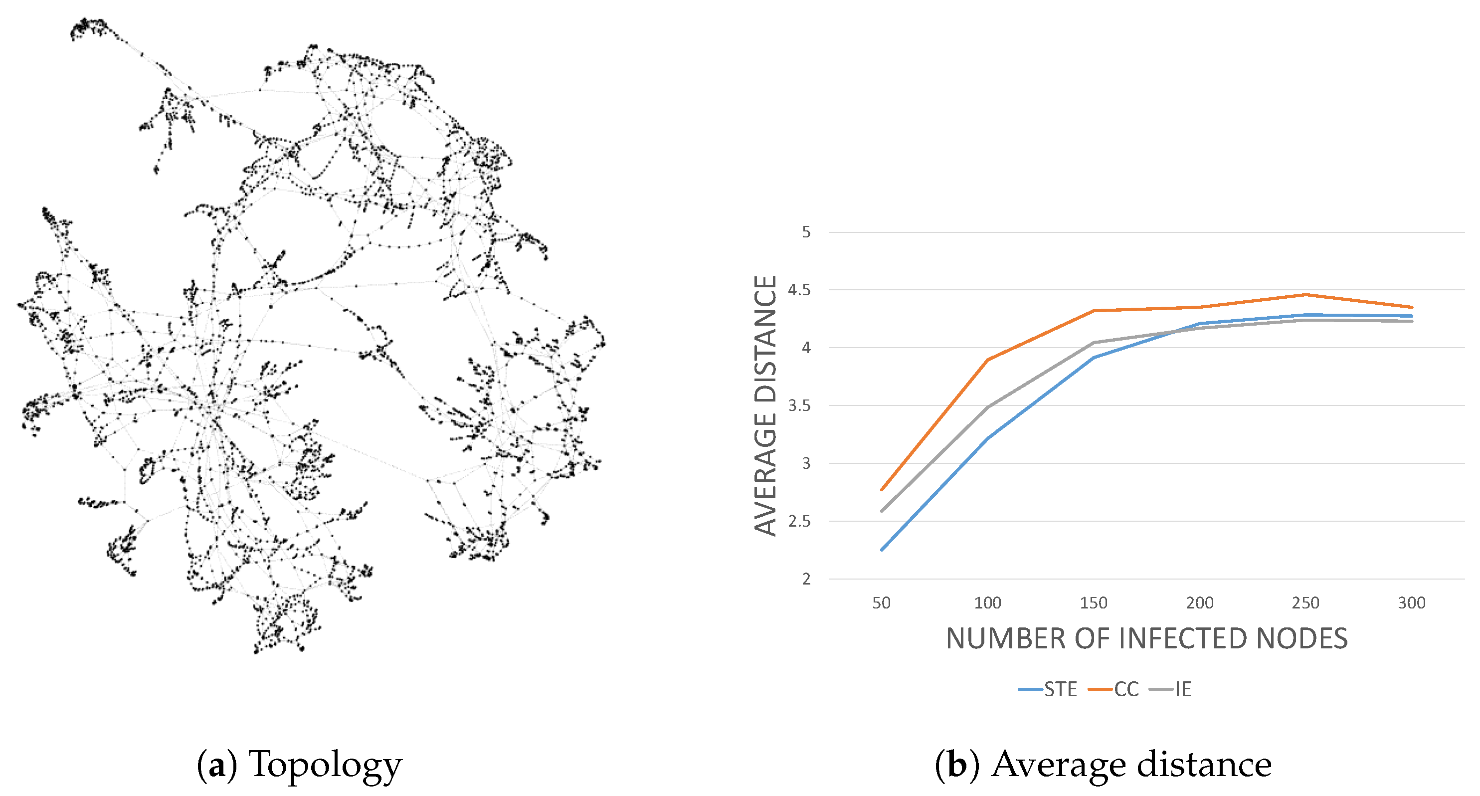
power grid network [
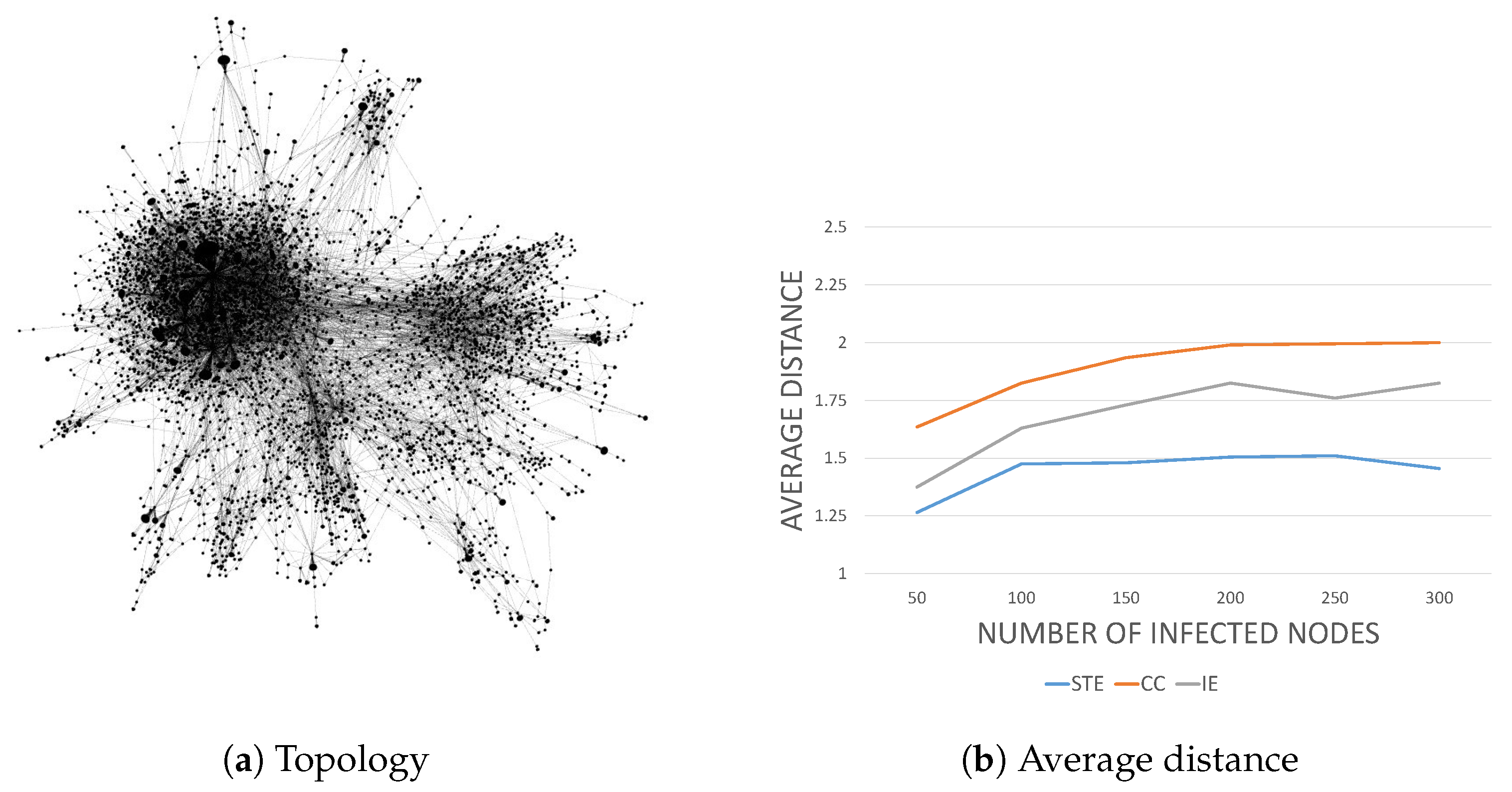
18]. The former, whose topology is shown in
Figure 7a, has more dense connectivity between the nodes than the latter, whose topology is depicted in
Figure 8a.
For the IAS network that consists of 6474 nodes and 13,895 edges, we chose an infection source and emulated the infection process. We conducted 200 simulations, varying the number of infected nodes. In the IAS network, STE clearly outperformed CC and IE, as shown in
Figure 7b.
For the power grid network that consists of 4941 nodes and 6594 edges, we repeated the simulations and obtained similar results, as shown in
Figure 8b, where STE outperformed CC and IE. However, unlike in the IAS network, their performance difference diminished as the number of infected nodes increased. We conjectured that this was because the power grid network was more sparsely connected than the IAS network. This is consistent with our results in
p-edge networks and
r-disk networks, where
r-disk networks were more densely-connected than
p-edge networks. The performance difference between CC, IE, and STE was outstanding in
r-disk networks compared to in
p-edge networks.


