Noise Reduction for High-Accuracy Automatic Calibration of Resolver Signals via DWT-SVD Based Filter

Abstract

High-accuracy calibration of resolver signals is the key to improve its angular measurement accuracy. However, inductive harmonics, residual excitation components, and random noise in signals dramatically restrict the further improvement of calibration accuracy. Aiming to reduce these unexpected noises, a filter based on discrete wavelet transform (DWT) and singular value decomposition (SVD) is designed in this paper. Firstly, the signal was decomposed into a time-frequency domain by DWT and several groups of coefficients were obtained. Next, the SVD operation of a Hankel matrix created from the coefficients was made. Afterwards, the noises were attenuated by reconstructing the signal with a few selected singular values. Compared with a conventional low-pass filter, this method can almost only preserve the fundamental and DC components of the signal because of the multi-resolution characteristic of DWT and the good correspondence between the singular value and frequency. Therefore, the calibration accuracy of the imperfect characteristics could be improved effectively. Simulation and experimental results demonstrated the effectiveness of the proposed method.

1. Introduction

The accurate information of the motor angular position is desired in high-performance servo control systems. Due to the simple structure, strong robustness, and adaptability to various harsh environments [1], resolvers have attracted great attention as shaft angle sensors in servo control applications such as antennas, radars, steering engines, and industrial robots.

Generally, a complete angular measurement system consists of a resolver and a Resolver-Digital Converter (RDC). In the software-based RDCs, the output signals of the resolver are transformed into sinusoidal and cosinusoidal envelopes with respect to the shaft angle after detection. Next, the angular position and velocity are obtained from the demodulation of envelopes [2]. However, there are usually some mechanical and electrical errors in a resolver. The former are caused by the manufacturing tolerance, assembled mismatch, and deformation. The latter result from winding nonlinearity, circuit asymmetry, and excitation signal distortion. Because of these errors, the envelopes contain five nonideal characteristics, such as amplitude imbalances, DC offsets, and imperfect quadrature [3], all of which seriously affect the accuracy of demodulation. Therefore, it is necessary to calibrate and correct the imperfect parameters in the resolver envelope signals.

As the calibration of the resolver signals is equivalent to the parameter estimation of non-orthogonal sinusoidal pair signals, approaches have been widely reported in recent years including a look-up table, optimization, observer, neural network, etc. An offline look-up table was constructed in Reference [4] to compensate the imperfectness in encoder signals. However, a trade-off has to be made between a larger table and increased sensitivity to noise. Heydemann [5] firstly proposed optimization approach by establishing a quadratic equation of five unknown parameters and obtained the optimal numerical solution by employing the least square method. Based on this, many literatures have presented improved methods [6,7]. However, the nonlinearity equation has multiple roots and lacks the ability to escape from local optimization if the initial iteration values are selected as unreasonable. To solve this issue, an adaptive estimator was given in Reference [8] that tracks the imperfect parameters of a characteristic ellipse formed by resolver signals. An automatic calibration algorithm based on state observer was introduced in Reference [9]. However, the strong coupling between parameters and the angular velocity in the mathematical model was undesired because the improvement of the calibration accuracy depended on the angular frequency. Therefore, an improved algorithm based on two-step gradient estimators was presented to decouple them [10]. Owing to the more accurate information of angular velocity, the calibration accuracy was further improved. Besides, signal flow network and deep learning algorithm in Reference [11] were introduced to ensure the independence of the variables.

However, the above methods are based on simplified models. The direct influence of inductive harmonics, residual excitation components, and random noise on the calibration accuracy was ignored. Since resolver windings are unevenly distributed and not exactly sinusoidal or cosinusoidal functions with respect to angular position, the output signals always contain harmonics [3]. Moreover, residual excitation components and random noise appear because of the excitation signal distortion and electrical errors from the conditioning circuit. These noises seriously limit the further improvement of the calibration accuracy no matter which method above is used.

Several studies on noise reduction have concerned themselves with improving the calibration accuracy. Common methods include mathematical modeling, filters, and phase-locked loop. Lara et al. [12] utilized a higher order approximation to describe harmonics but had a slight convergence deviate. The smaller the deviation was, the more complex model needed to be established. Shang et al. [13] analyzed the harmonics by Fourier transform and weakened the 3rd harmonic through adding a corresponding harmonic in the shape function of the rotor structure. Obviously, it required a special rotor structure. Similarly, the error profile curve with respect to the angle was described by Fourier series [14]. However, it was not an automatic calibration. Finite Impulse Response filter was applied in a self-tuning circuit [15], which reduced noise but had an inherent time delay and phase distortion. An adaptive phase-locked loop proposed in Reference [16] was able to filter noise online to a certain extent. However, the continuous calibration increased the unnecessary delay with the errors supposed constant in a short time. Another novel RDC algorithm performed in a frequency domain was studied in Reference [17]. Since the detection was unrequired and only the carrier frequency component was utilized to estimate parameters, it was preferable to suppress the disturbances outside of the carrier frequency. However, the amplitude imbalances were out of consideration.

In order to achieve high-accuracy calibration of the imperfect parameters, it is important to reduce the three types of noises. Some image noising methods are worth learning and using for reference. The discrete wavelet transform (DWT) has been widely used to signal or image denoising. Because of the characteristic of multi-resolution, DWT can distinguish noise and useful information to different frequency bands [18,19,20]. But the conventional wavelet threshold denosing method [21] is difficult to flexibly select a reasonable threshold and has little effectiveness in noise reduction near the fundamental wave. Moreover, nonlocal self-similarity prior learning [22], convolutional neural network [23], and singular value decomposition (SVD) [24] are also used in image denoising. Guo et al. [24] used a few large singular values and corresponding singular vectors to estimate the image and reduce noise. Recently, because of the multi-resolution characteristic of DWT and the good correspondence between the singular value and frequency, the cooperation between DWT and SVD [25,26] in the time-frequency domain has attracted the attention of researchers. At present, several different combinations have been adopted in image watermarking [27], image contrast enhancement [28], image compression and denoising [29], and the feature extraction of signals [30].

Aiming to reduce the noises and obtain the high calibration accuracy of resolver signals, a DWT-SVD based filter in time-frequency domain is designed in this paper. Since this method is able to reduce inductive harmonics, residual excitation components, and random noise in resolver signals with only the fundamental and DC components being retained, the calibration accuracy can be improved effectively. Simulation and experimental results verify the effectiveness of the proposed method.

This paper is organized as follows: The calibration principle of resolver signals is introduced and the problem of noises is formulated in Section 2. Section 3 presents the designed DWT-SVD based filter and describes the filtering processing in detail. To verify the effectiveness of the method, simulation and experimental results are analyzed in Section 4. Finally, the concluding remarks are given in Section 5.

2. Calibration Principle and Problem Formulation of Resolver

As shown in Figure 1, in a software-based RDC, when the rotor winding of resolver is excited with a high frequency voltage, the two spatially orthogonal windings on the stator will produce amplitude modulation signals which have sinusoidal and cosinusoidal envelopes with respect to shaft angle. Then the envelopes are obtained from detection. Finally, owing to the mathematical properties of trigonometric function, the angular position $\theta$ and velocity $\omega$ are calculated from envelopes by phase-locked loop, arctangent or other demodulation algorithms.

In practice, the resolver signals after detection are always disturbed by imperfect characteristics. The amplitude imbalances and DC offsets result from the eccentric rotor, unequal winding, and asymmetric circuit. The imperfect quadrature arises when the space angle of two coils on stator are not exactly equal to $\pi /2$. Therefore, the envelopes should be described as

$$\{\begin{array}{l}{y}_s=a_{s1}\sin \theta +a_{s0}\\ y_c=a_{c1}\cos (\theta +\beta )+a_{c0}\end{array}$$

(1)

where $a_{s1}$ and $a_{c1}$ are the amplitudes, $a_{s0}$ and $a_{c0}$ are the offsets, $\beta$ represents the imperfect quadrature. Obviously, it is necessary to calibrate the envelopes and correct (1) to the standard form of sine and cosine functions before demodulation.

The calibration of resolver signals is a process of estimating the five imperfect parameters of non-orthogonal sinusoidal pair signals. These estimation methods have been widely reported in recent years. By using a look-up table, optimization, observer, neural network or other estimation algorithm, the imperfect parameters can be estimated to correct and reduce demodulation error. Thereafter, the signals can be calibrated by substituting the estimated value into the following equation:

$$\{\begin{array}{l}{\widehat{y}}_s=(y_s-{\widehat{a}}_{s0})/{\widehat{a}}_s=\sin \theta \\ {\widehat{y}}_c=(y_c-{\widehat{a}}_{c0})/{\widehat{a}}_c\cos \beta +(y_s-{\widehat{a}}_{s0})tan\beta /{\widehat{a}}_s=\cos \theta \end{array}.$$

(2)

Unfortunately, most calibration algorithms are based on simplified models and ignore the noises like harmonics, residual excitation components, and random noise in envelopes, all of which seriously affect the calibration of the resolver. The harmonic distortion arises when the unevenly distributed windings are not exactly sinusoidal or cosinusoidal shaped with respect to the angular position. The residual excitation components and random noise exist due to the electrical errors from conditioning circuit. Hence, the Equation (1) can be rewritten in the following manner:

$$\{\begin{array}{l}{y}_s=a_{s0}+a_{s1}\sin \theta +{\displaystyle \sum _{n=2}^{\infty }{a}_{sn}\sin n\theta }+d_s\\ y_c=a_{c0}+a_{c1}\cos (\theta +\beta )+{\displaystyle \sum _{n=2}^{\infty }{a}_{cn}\cos n\theta +d_c}\end{array}$$

(3)

where $n$ is the harmonic order, $a_{sn}$ and $a_{cn}$ represent the amplitudes of the $n\mathrm{th}$ harmonic, $d_s$ and $d_c$ are random noise.

As shown in Figure 1, aiming at suppressing noises and improving calibration accuracy, several methods including mathematical modeling and low-pass filter have been used recently. However, the mathematical modeling method makes an inevitable deviation and is pretty complex. The low-pass filter has an inherent phase distortion and cannot attenuate the noises in the passband. Therefore, it is still a serious problem to filter the noises without phase distortion and preserve the fundamental and DC component only.

3. Design of DWT-SVD Based Filter

In order to reduce the three types of noises in resolver signals without phase distortion and preserve the fundamental and DC component only, a DWT-SVD based filter is designed in this paper. As shown in Figure 2, this method is divided into 3 steps: (1) Decompose the resolver envelopes into several groups of coefficients corresponding to different frequency bands through DWT; (2) Process the coefficients by SVD to filter noise; (3) The filtered envelopes are reconstructed with the processed coefficients. Since the procedure of the sinusoidal pair signals are identical, the following only considers the sinusoidal envelope $y_s$ in Equation (3).

3.1. Signal Decomposition

The first step is to decompose the signal into approximation coefficients and detail coefficients through J-layer DWT. Actually, the essence of DWT can be regarded as a process of utilizing a set of high-pass and low-pass filters on the signal. Furthermore, the high-pass and low-pass filters depend on the selected wavelet base function. Thus, the approximation coefficients $ca$ which represented low frequency information and detail coefficients $cd$ which represented high frequency information are obtained. In this method, the Mallat algorithm is employed to achieve J-layer DWT. The coefficients $ca$ and $cd$ of each layer are calculated as follows:

$$\{\begin{array}{l}c{a}_j(k)={\displaystyle \sum _{n}h(n-2k)c{a}_{j-1}(n)}\\ c{d}_j(k)={\displaystyle \sum _{n}g(n-2k)c{a}_{j-1}(n)}\end{array},j=1,2,3,\cdots ,J$$

(4)

where h and g represent the impulse responses of low-pass filter and high-pass filter, respectively, when $j=1$, $c{a}_{j-1}$ represents the envelope signal of resolver.

The procedure of multi-layer decomposition is shown in Figure 3. Assuming the sampling frequency $f_s$ satisfies the Nyquist Sampling Theorem and the total layer is J, the spectrum of the signal is limited in $(0~f_s/2)$ according to the normalized frequency band. Due to the multi-resolution characteristic of DWT, the frequency band of $c{d}_1$, $c{d}_2$ and $c{d}_3$, respectively, are $(f_s/4~f_s/2)$, $(f_s/8~f_s/4)$, $(f_s/16~f_s/8)$. And, more remarkably, $c{a}_3$ is in the low frequency band $(0~f_s/16)$ which contains the fundamental and DC components of resolver envelope. If the layer J is too small, the data length of $c{a}_J$ would be overmuch and then increase the computational complexity of SVD. Otherwise, the useful information would leak into the detail coefficients. Therefore, selecting the layer reasonably would directly determine whether the $c{a}_J$ includes a fundamental wave. Moreover, it is important to make the detail coefficients possess harmonics and residual excitation components as far as possible.

3.2. Coefficient Processing

The second step is to analyze the approximation coefficient $c{a}_J$ and detail coefficients from $c{d}_1$ to $c{d}_J$. Since the detail coefficients contain residual excitation components and some harmonics with so little useful information, they can be addressed by forced noise reduction. The coefficient $c{a}_J$, which involves the fundamental wave, is still affected by noises, such as random noise and harmonics. Therefore, SVD is employed to reduce these noises.

The SVD of a matrix $\mathit{H}\in R^{m\times n}$ is defined as the following equation:

$$\mathit{H}=\mathit{U}\mathit{S}{\mathit{V}}^T$$

(5)

where $\mathit{U}\in R^{m\times m}$ and $\mathit{V}\in R^{n\times n}$ are orthogonal matrices. The diagonal matrix $\mathit{S}\in R^{m\times n}$ can be given by

$$\mathit{S}=(diag({\sigma }_1,{\sigma }_2,\cdots ,{\sigma }_p),\mathit{O})$$

(6)

where $p=\min (m,n)$ is the number of singular values, and ${\sigma }_i(i=1,2,\cdots p)$ represent the singular values of matrix $\mathit{H}$ which satisfy ${\sigma }_1\ge {\sigma }_2\ge \cdots \ge {\sigma }_p>0$.

As $c{a}_J=(x_1,x_2,\cdots ,x_N)$ is a one-dimension data, a Hankel matrix $\mathit{H}$ needs to be construct when processing $c{a}_J$ by SVD. The matrix can be expressed as

$$\mathit{H}={\left[\begin{array}{cccc}{x}_1& x_2& \cdots & x_{N-n+2}\\ x_2& x_3& \cdots & x_{N-n+2}\\ ⋮& ⋮& \ddots & ⋮\\ x_{N-n+1}& x_{N-n+2}& \cdots & x_N\end{array}\right]}_{m\times n}$$

(7)

where n satisfies $1<n<N$ and $m=N-n+1$. From Equation (7) each row vector in the Hankel matrix lags only one data behind the previous row vector, which means the adjacent row vectors are highly correlated with useful information and independent of noises. Therefore, the fundamental and DC components of the signal which contain the main energy will be concentrated in a few large singular values. Due to the good correspondence between the singular value and frequency, the first two maximum values represent the fundamental wave, and the value which represents the DC component can be selected from test. According to the principle, the modified $c{a}_J^{\prime }$ can be calculated from Equation (5) by using only three singular values.

3.3. Signal Reconstruction

The last step is reconstruction. The procedure of multi-layer wavelet reconstruction is shown in Figure 4. The formula of reconstruction is given by

$$c{a}_{j-1}^{\prime }(n)={\displaystyle \sum _k{h}^{*}(n-2k)c{a}_j^{\prime }(k)}+{\displaystyle \sum _k{g}^{*}(n-2k)c{d}_j^{\prime }(k)}.$$

(8)

Since the detail coefficients are forced to be zero, the envelope signal of resolver is reconstructed with the modified approximation coefficient $c{a}_J$. Finally, the signals of resolver after noise reduction are obtained.

From the above description, it can be seen that the filter can reduce the harmonics, residual excitation components, and random noise and extract the fundamental and DC components of resolver envelopes without phase distortion.

4. Simulation and Experimental Results

Aiming to evaluate the performance of the proposed method, the spectrums of signals are compared among the following four groups both in simulation and experiment.

Group 1: The original signals;

Group 2: The signals denoised by the low-pass Butterworth filter;

Group 3: The signals denoised by the DWT based filter;

Group 4: The signals denoised by the DWT-SVD based filter.

Next, in order to verify the influence of the filter on the calibration accuracy, the imperfect parameters of the above signals are estimated by an automatic calibration algorithm based on two-step gradient estimators in Reference [10]. The simulation and experimental results are analyzed as follows.

4.1. Simulation Results

In the simulation, sinusoidal pair signals are generated to simulate the envelopes of resolver. The angular frequency ω is $2\pi \mathrm{rad}/\mathrm{s}$. The imperfect parameters are set as $a_{s1}=1.8370\mathrm{V}$, $a_{s0}=0.1365\mathrm{V}$, $a_{c1}=1.9520\mathrm{V}$, $a_{c0}=0.1452\mathrm{V}$ and $\beta =1.2°$. The harmonics are shown in

Table 1. Harmonics in signals.

Order	2	3	4	5
$y_s$ (V)	0.0255	0.0130	0.0078	0.0032
$y_c$ (V)	0.0243	0.0128	0.0082	0.0025

. In addition, the residual excitation components are 0.0010 V and 0.0011 V, respectively, with the frequency being 10 kHz. The SNR of signals is 35 dB by adding Gaussian white noise. The simulation is proceeded by using MATLAB.

In the DWT-SVD based filter (Group 4), a biorthogonal wavelet basis function “bior 5.5” is chosen. Since the biorthogonal wavelet has a linear phase, the signals can be completely reconstructed without phase distortion. Whereby, the layer of wavelet decomposition is 4. As comparisons, the low-pass Butterworth filter in Group 2 is designed with no more than 0.1 dB of ripple in a passband from 0 to 3 Hz, and at least 30 dB of attenuation in the stopband. The DWT based filter in Group 3 is designed by using 6-layer wavelet decomposition and reconstruction to reduce the high-frequency noise.

The calibration method in Reference [10] is constructed as

$$\{\begin{array}{l}\dot{x}=\xi +y_s\hfill \\ \dot{\xi }=-{\lambda }_{0}x-{\lambda }_1(\xi +y_s)\hfill \\ \dot{\eta }=k[x^2({\lambda }_0-{\widehat{\omega }}^2)+({\lambda }_{1}x+y_s)(\xi +y_s)]\hfill \\ {\widehat{\omega }}^2=\eta -kx{y}_s\hfill \\ {\dot{\widehat{a}}}_0=\gamma (y_s-{\widehat{y}}_s)\hfill \\ {\dot{\widehat{a}}}_1=\gamma \sin \widehat{\omega }t(y_s-{\widehat{y}}_s)\hfill \\ {\dot{\widehat{a}}}_2=\gamma \cos \widehat{\omega }t(y_s-{\widehat{y}}_s)\hfill \\ {\widehat{y}}_s={\widehat{a}}_0+{\widehat{a}}_1\sin \widehat{\omega }t+{\widehat{a}}_2\cos \widehat{\omega }t\hfill \end{array}$$

(9)

where the estimator gains are chosen as $k=100,{\lambda }_0=15,{\lambda }_1=15,\gamma =0.8$. The angular velocity $\widehat{\omega }$ is estimated by the first four equations. Then, the amplitude ${\widehat{a}}_{s1}=\sqrt{{\widehat{a}}_1^2+{\widehat{a}}_2^2}$, DC offset ${\widehat{a}}_{s0}={\widehat{a}}_0$ and phase ${\widehat{\varphi }}_s={\tan }^{-1}({\widehat{a}}_2/{\widehat{a}}_1)$ of $y_s$ can be estimated by the rest of equations. Since the procedure of $y_c$ is same as $y_s$, phase shift is calculated by $\widehat{\beta }={\widehat{\varphi }}_s-{\widehat{\varphi }}_c$.

The results are analyzed as follows:

(1) As shown in Figure 5, the detail coefficients $c{d}_1~c{d}_4$ of $y_s$ reflect noises with no useful information. In contrast, the approximation coefficient $c{a}_4$ contains the information of fundamental and DC components with a few harmonics and noises. Thus the decomposition can be understood as a pre-filter. Then SVD operation of a Hankel matrix created from $c{a}_4$ is made. The singular values are given in

Table 2. Partial singular values of approximation coefficient $c{a}_4$.

Number	1	2	3	4	5
Value	6896.7	6893.6	1026.7	95.2	95.1

. It is obvious that the 1st and 2nd singular values represent the fundamental wave and the 3rd reflects the DC components. Therefore, $y_s$ can be finally reconstructed from the new $c{a}_4^{\prime }$ which is calculated by the three singular values.

(2) The performance of the filter can be verified from spectral analysis. As shown in Figure 6, the spectrum of the original signal includes harmonics and noises. However, the low-pass filter is unable to reduce noises in the passband and results in a slight amplitude attenuation of fundamental wave. The DWT based filter has no effect on fundamental wave but is unable to suppress low-order harmonics. Unlike these filters, it is showed obviously in Figure 6d that the DWT-SVD filter retains almost only the fundamental and DC components.

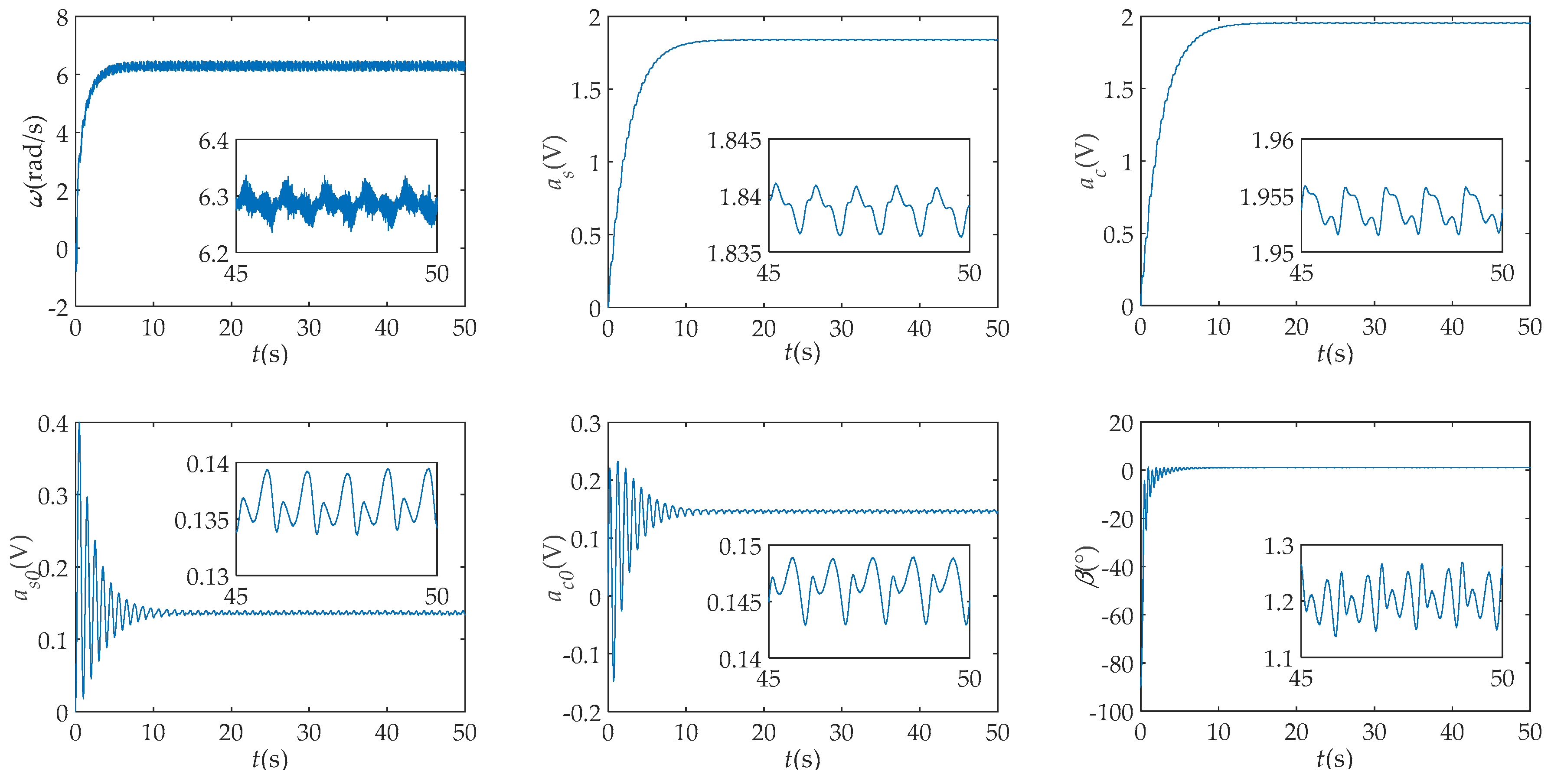
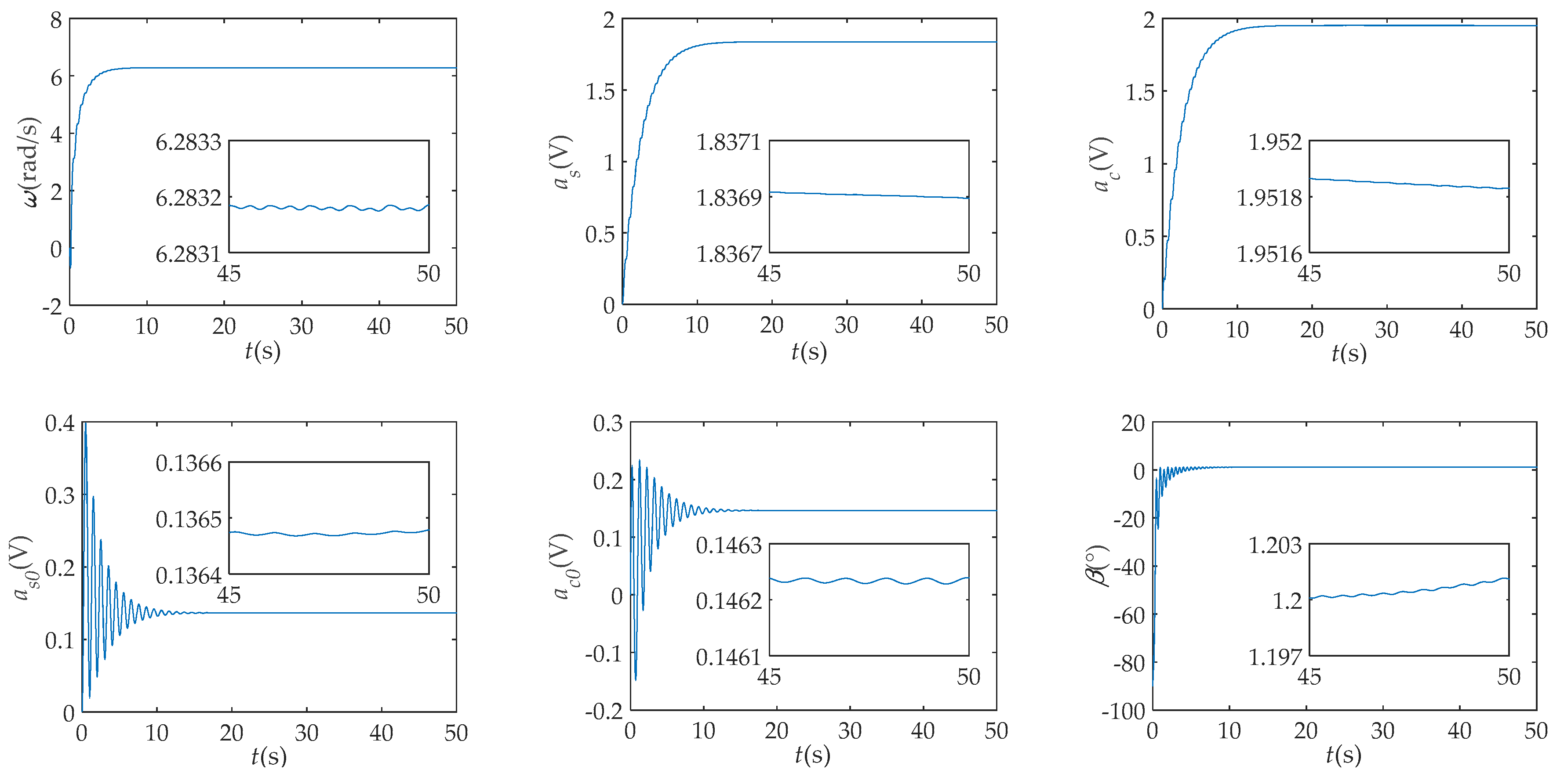
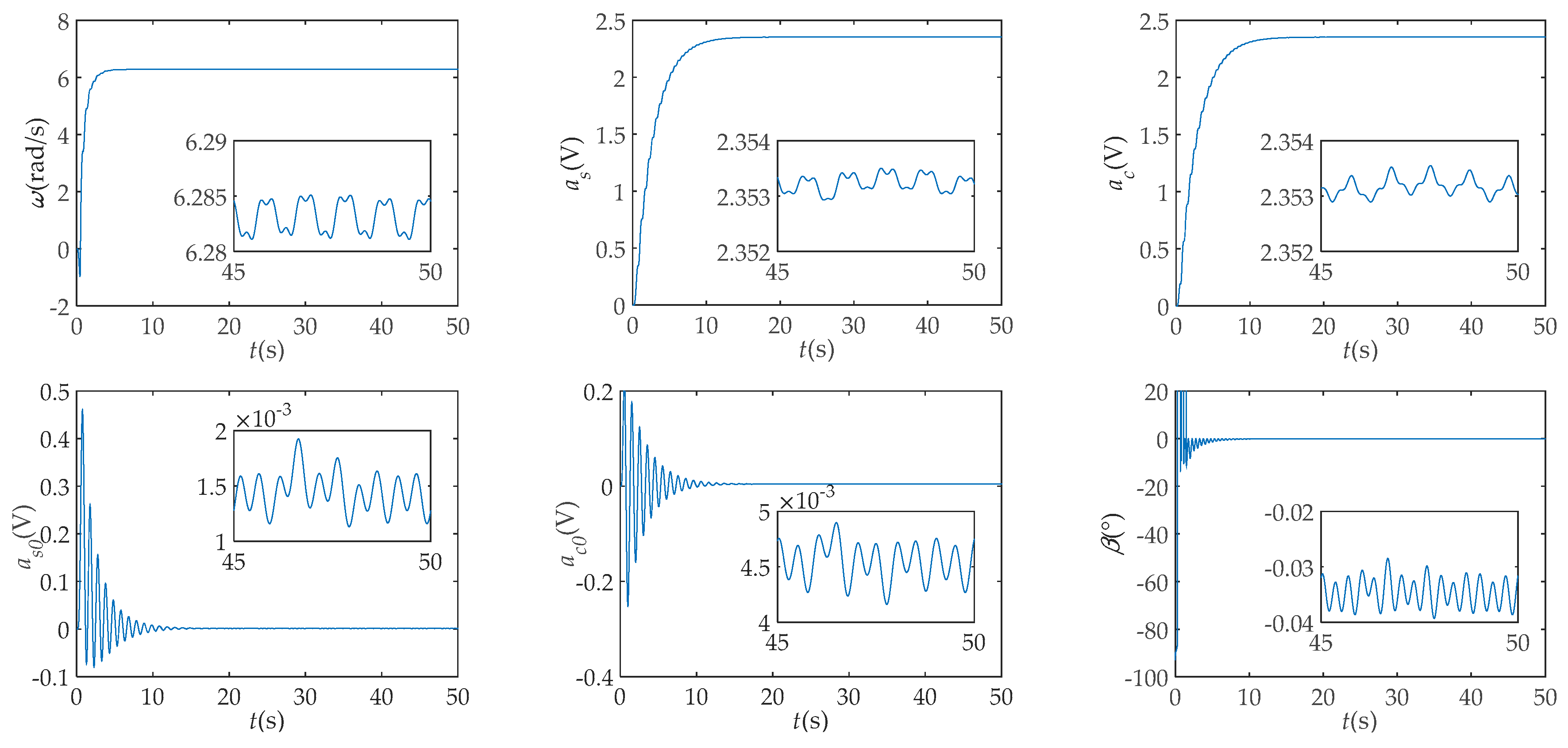
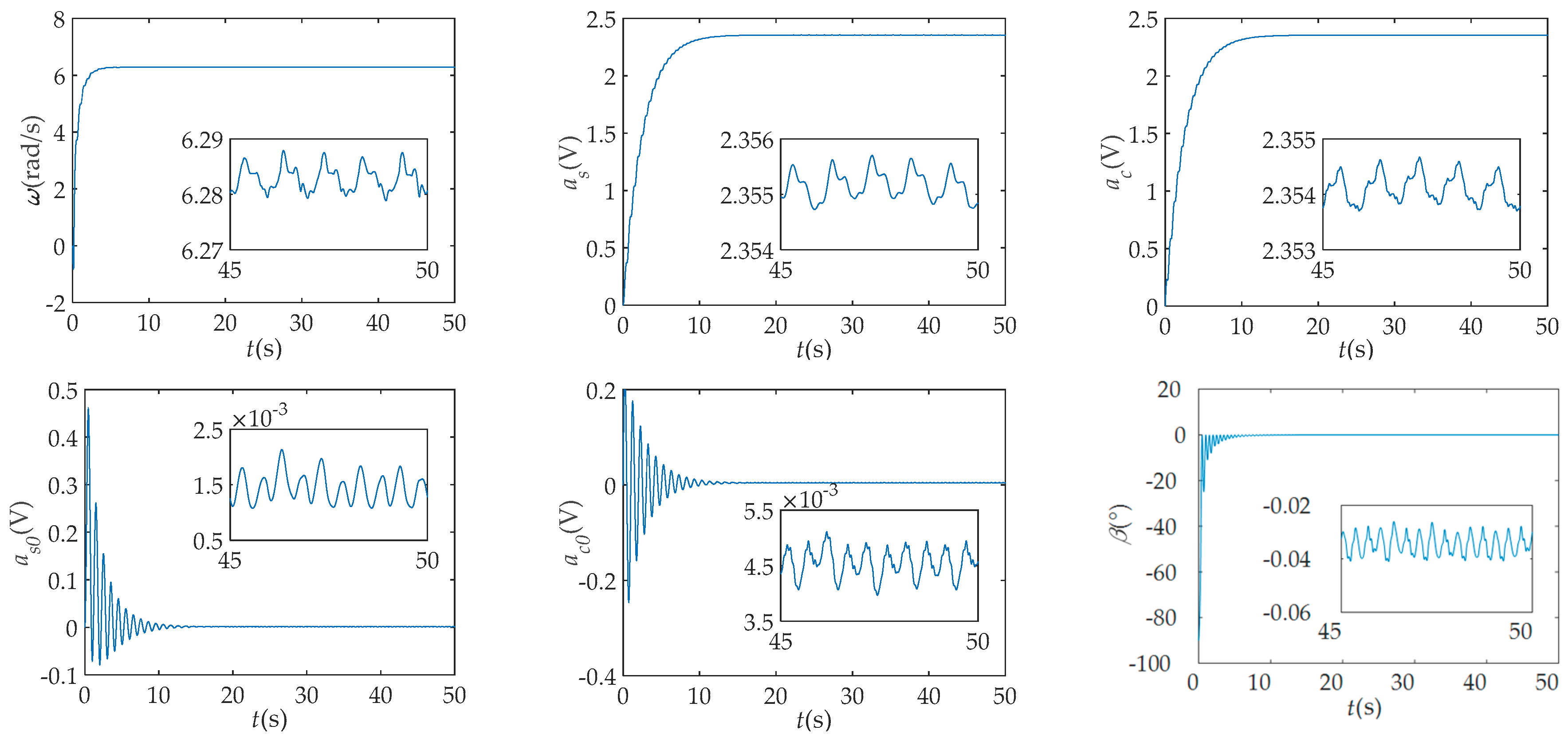
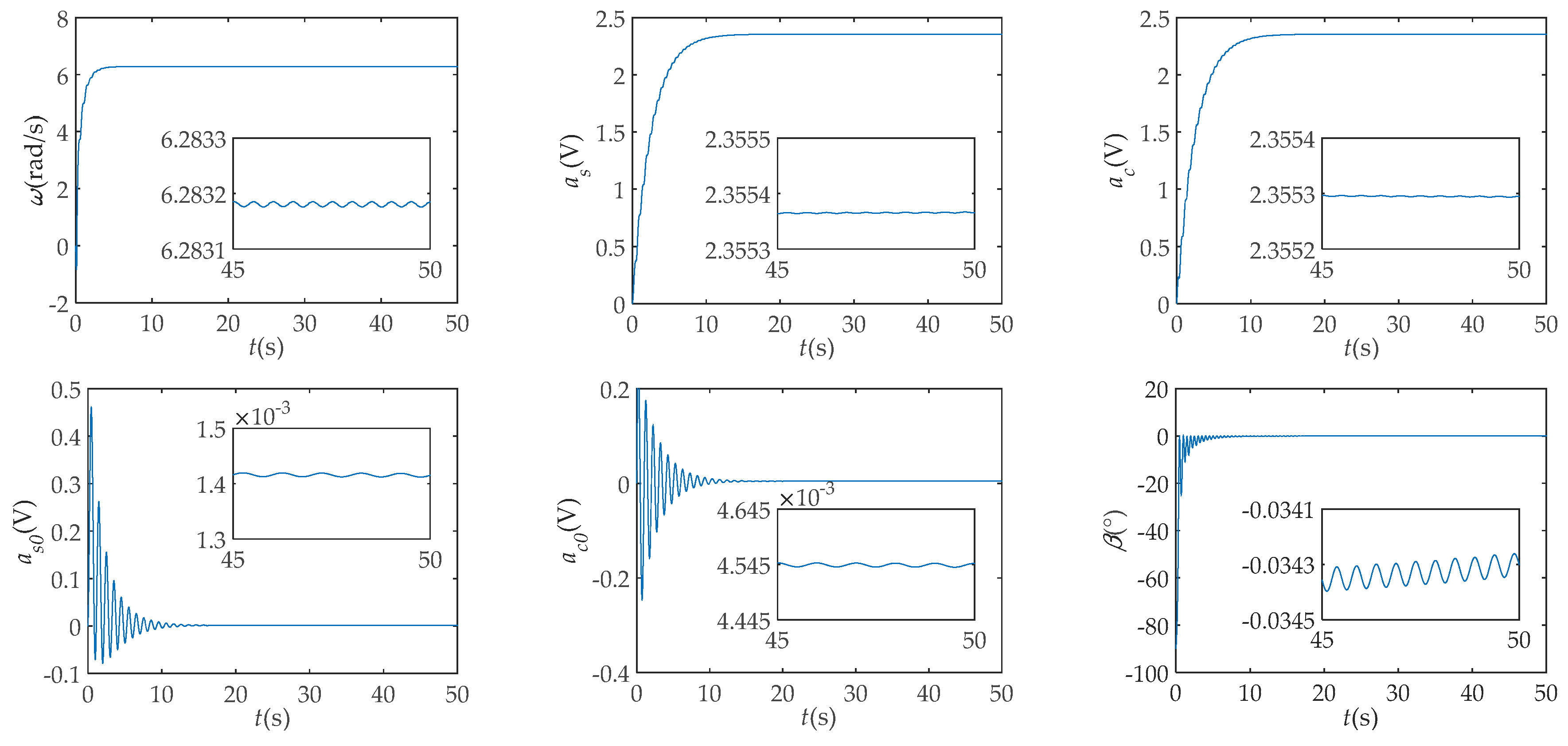
(3) By the calibration algorithm in Reference [10], the estimations of the angular frequency and five imperfect parameters in Groups 1–4 are given in Figure 7, Figure 8, Figure 9 and Figure 10, respectively. And

Table 3. Results of calibration in simulation.

Parameters		$\mathit{\omega }(\mathbf{rad}/\mathbf{s})$	${\mathit{a}}_{\mathit{s}}(\mathbf{V})$	${\mathit{a}}_{\mathit{c}}(\mathbf{V})$	${\mathit{a}}_{\mathit{s}0}(\mathbf{V})$	${\mathit{a}}_{\mathit{c}0}(\mathbf{V})$	$\mathit{\beta }{(}^{°})$
Preset values		6.283185	1.83700	1.95200	0.13650	0.14520	1.2000
Calibrated directly	Estimates	6.285769	1.83893	1.95372	0.13643	0.14632	1.2019
	STD	1.20 × 10−2	1.25 × 10−3	1.26 × 10−3	1.63 × 10−3	1.63 × 10−3	3.02 × 10−2
After the Butterworth filter	Estimates	6.283505	1.83577	1.95035	0.13644	0.14631	1.2017
	STD	5.20 × 10−3	7.32 × 10−4	7.00 × 10−4	7.54 × 10−4	6.95 × 10−4	1.48 × 10−2
After the DWT	Estimates	6.283640	1.83741	1.95210	0.13644	0.14632	1.2019
	STD	1.01 × 10−2	1.22 × 10−3	1.23 × 10−3	1.25 × 10−3	1.18 × 10−3	2.55 × 10−2
After the designed filter	Estimates	6.283179	1.83691	1.95187	0.13648	0.14623	1.2002
	STD	2.49 × 10−6	1.11 × 10−5	2.28 × 10−5	4.59 × 10−6	3.44 × 10−6	4.23 × 10−4

shows the estimated results calculated by means of the data and the standard deviations (STD) in the range of 40–50 s. From Figure 7, Figure 8, Figure 9 and Figure 10, the steady-state error of Group 4 is smaller than that of the other groups. Compared with the preset values in Table 3, the accuracy of ω after the designed filter reaches ${10}^{-5}\mathrm{rad}/\mathrm{s}$, while the accuracies of the other groups are ${10}^{-3}\mathrm{rad}/\mathrm{s}$, ${10}^{-4}\mathrm{rad}/\mathrm{s}$ and ${10}^{-4}\mathrm{rad}/\mathrm{s}$, respectively. The accuracy of amplitudes after the designed filter reaches to ${10}^{-4}\mathrm{rad}/\mathrm{s}$, while the others are ${10}^{-3}\mathrm{rad}/\mathrm{s}$ and Group 2 has a slight attenuation. Moreover, the STD is reduced at least two orders of magnitude more than the other groups. It is worth noting that the designed filter leads to a high-accuracy phase due to the phase undistorted characteristic, while the low-pass filter causes a phase shift. Therefore, the DWT-SVD filter apparently improves the calibration accuracy and is more stable than other ways.

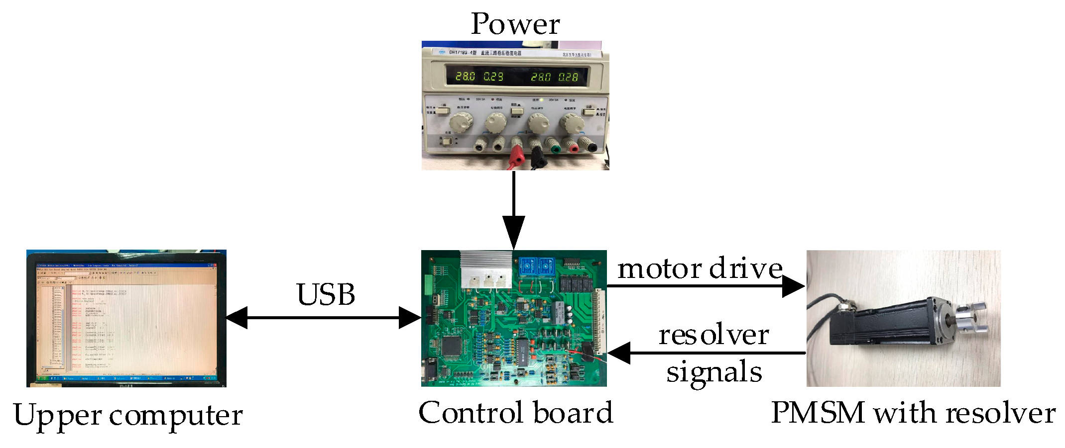
4.2. Experimental Results

The experimental platform is shown in Figure 11. A control board drives a permanent magnet synchronous motor (PMSM) and a resolver (Infranor, Zurich, Switzerland). The parameters of PMSM and resolver are given in

Table 4. PMSM and resolver parameters.

PMSM		Resolver
Pole pairs	2	Pole pairs	1
Rated voltage	110 V(AC)	Input voltage	5 V ± 0.2 V (AC)
Rated speed	3000 r/min	Input frequency	10 kHz
Torque constant	0.15 Nm/A	Output voltage	>2 V
Phase resistance	8 Ω	Transformer ratio	0.5 ± 5%
Phase inductance	10 mH	Electrical error	$\le 10^{\prime }$

. In this experiment, PMSM is driven to rotate at $\omega =2\pi \mathrm{rad}/\mathrm{s}$ and the resolver measures its angular position. After envelope detection circuits, the envelops of resolver output signals are uploaded to the upper computer through USB. Then the envelops are denoised and calibrated in the upper computer.

In this experiment, the parameters of four groups are set the same as in the simulation. The results are analyzed as follows:

(1) The coefficients and singular values of $y_s$ calculated from the DWT-SVD based filter are given in Figure 12 and

Table 5. Partial singular values of approximation coefficient $c{a}_4$ in experiment.

Number	1	2	3	4	5	6	7
value	9418.9	9410.4	19.8	19.7	11.7	9.3	9.2

. From Figure 12, the approximation coefficient $c{a}_4$ has already pre-filtered the residual excitation components and most of the random noise. Next, according to a rigorous test, the 1st and 2nd singular values in Table 5 reflect the fundamental wave and the 5th value reflects the DC components. Finally, the signal can be reconstructed by the three singular values and corresponding singular vectors.

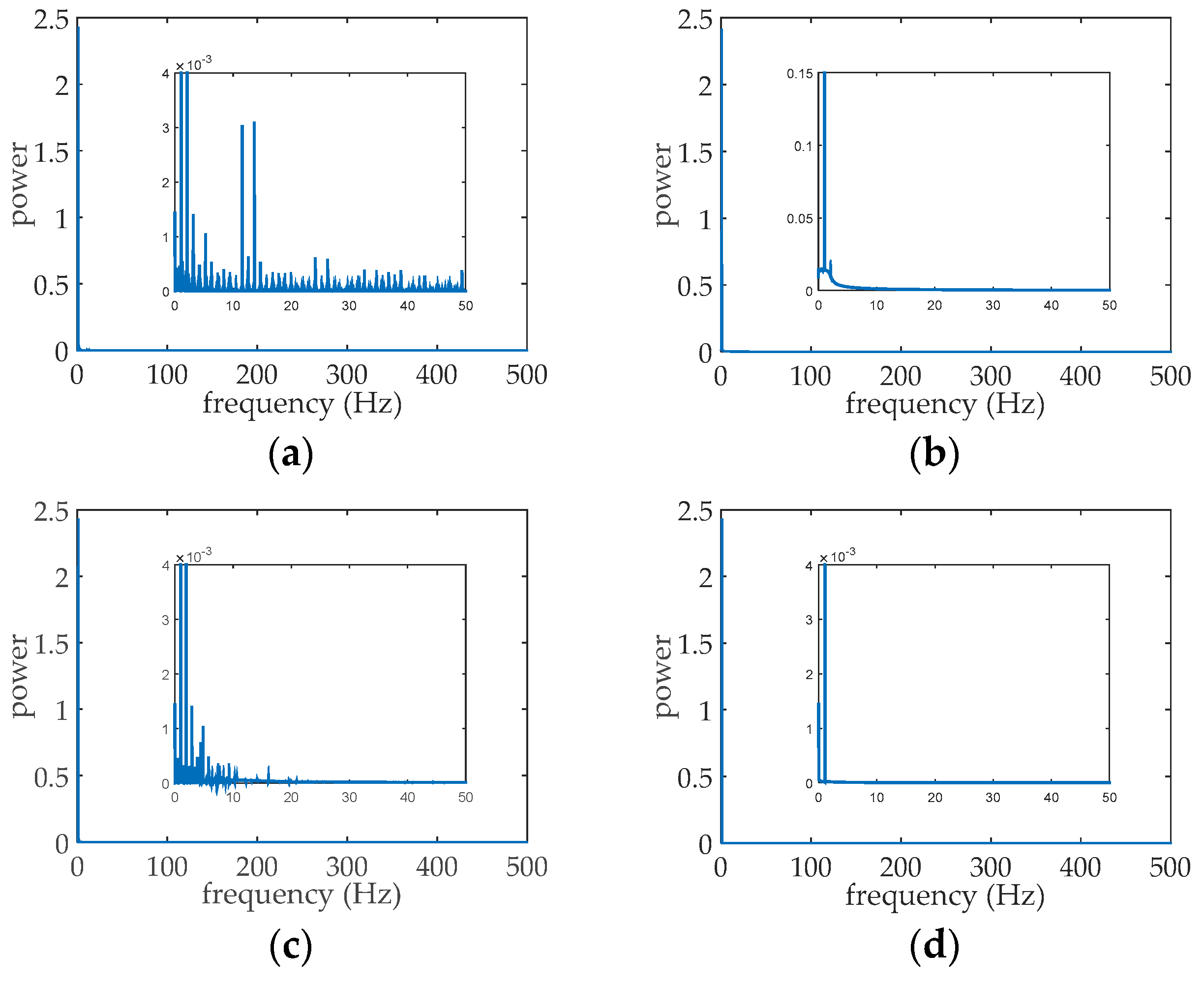
(2) The spectrums in Figure 13 also verify the performance of the designed filter. As shown in Figure 13a, the spectrum of the original signal contains harmonics and random noise. However, the spectrum in Figure 13b shows that the low-pass filter attenuates the DC component seriously and cannot reduce noise in the passband. The spectrum in Figure 13c shows that the DWT-based filter is unable to suppress low-order harmonics although it can reduce the high-frequency noise. Compared with Groups 1–3, the DWT-SVD filter in Group 4 preserves almost only the fundamental and DC components.

(3) As show in Figure 14, Figure 15, Figure 16 and Figure 17 and

Table 6. Results of calibration in experiment.

Parameters		$\mathit{\omega }(\mathbf{rad}/\mathbf{s})$	${\mathit{a}}_{\mathit{s}}(\mathbf{V})$	${\mathit{a}}_{\mathit{c}}(\mathbf{V})$	${\mathit{a}}_{\mathit{s}0}(\mathbf{V})$	${\mathit{a}}_{\mathit{c}0}(\mathbf{V})$	$\mathit{\beta }{(}^{°})$
Calibrated directly	Estimates	6.28288	2.3551	2.3550	1.446 × 10−3	4.548 × 10−3	−0.03450
	STD	2.88 × 10−3	2.54 × 10−4	2.56 × 10−4	2.85 × 10−4	2.86 × 10−4	3.99 × 10−3
After the Butterworth filter	Estimates	6.28304	2.3532	2.3532	1.445 × 10−3	4.545 × 10−3	−0.03462
	STD	1.80 × 10−3	1.54 × 10−4	1.57 × 10−4	1.70 × 10−4	1.66 × 10−4	2.44 × 10−3
After the DWT	Estimates	6.28299	2.3552	2.3541	1.447 × 10−3	4.547 × 10−3	−0.03448
	STD	2.19 × 10−3	2.48 × 10−4	2.53 × 10−4	2.56 × 10−4	2.57 × 10−4	3.83 × 10−3
After the designed filter	Estimates	6.28318	2.3553	2.3532	1.416 × 10−3	4.544 × 10−3	−0.03436
	STD	3.30 × 10−6	7.99 × 10−6	1.07 × 10−7	2.48 × 10−6	2.54 × 10−6	4.16 × 10−5

, the estimations of the angular frequency ω and five imperfect parameters $a_{s1}$, $a_{c1}$, $a_{s0}$, $a_{c0}$ and $\beta$ in Groups 1–4 are carried out by the calibration algorithm in [10], respectively. From Figure 14, Figure 15, Figure 16 and Figure 17, the steady-state errors in Groups 1 and 3 are in the same order of magnitude while in Group 2 is smaller, since the harmonics in Group 2 is weaker than Groups 1 and 3. Compared with them, Group 4 has the smallest steady-state error among the four groups because the proposed method can suppress harmonics effectively. In order to further verify the effectiveness of the proposed method, Table 6 gives the STDs of estimated parameters, which are calculated from the data in the range of 40–50 s. The STD is an important index to compare the four groups while the true values are unknown. From Table 6, it is obvious that Group 4 has the smallest STDs which are reduced at least two orders of magnitude than others.

5. Conclusions

In order to improve the calibration accuracy of the resolver signals, a DWT-SVD based filter was designed in this paper to reduce the noises. Most of the noises in the resolver, such as the inductive harmonics, residual excitation components, and random noise were taken into account. Firstly, the resolver signals were decomposed to the approximation coefficient and detail coefficients by DWT. The decomposition pre-filtered the residual excitation components and part of the noises. Next, the singular values of approximation coefficient were calculated. Finally, the signals were reconstructed by a few selected singular values to suppress harmonics and preserve almost only the fundamental and DC components. Because of the multi-resolution characteristic of DWT and the good correspondence between the singular value and frequency, this method is favorable to dramatically reduce the noises. Therefore, the proposed filter improved the calibration accuracy of the nonideal parameters, such as amplitude deviations, DC offsets, and imperfect quadrature in resolvers. The effectiveness of the designed filter was verified by simulation and experimental results.

References

1. Alipour-Sarabi, R.; Nasiri-Gheidari, Z.; Tootoonchian, F.; Oraee, H. Performance analysis of concentrated wound-rotor resolver for its applications in high pole number permanent magnet motors. IEEE Trans. Ind. Electron. 2017, 17, 7877–7885. [Google Scholar] [CrossRef]
2. Liu, H.; Wu, Z. Demodulation of angular position and velocity from resolver signals via Chebyshev filter-based type III phase locked loop. Electronics 2018, 7, 354. [Google Scholar] [CrossRef]
3. Hanselman, D.C. Resolver signal requirements for high accuracy resolver-to-digital conversion. IEEE Trans. Ind. Electron. 1991, 37, 556–561. [Google Scholar] [CrossRef]
4. Tan, K.K.; Zhou, H.X.; Lee, T.H. New interpolation method for quadrature encoder signals. IEEE Trans. Instrum. Meas. 2002, 51, 1073–1079. [Google Scholar] [CrossRef]
5. Heydemann, P.L.M. Determination and correction of quadrature fringe measurement errors in interferometers. Appl. Opt. 1981, 20, 3382–3384. [Google Scholar] [CrossRef] [PubMed]
6. Balemi, S. Automatic calibration of sinusoidal encoder signals. In Proceedings of the 16th Triennial World Congress, Prague, Czech Republic, 3–8 July 2005; pp. 1189–1195. [Google Scholar]
7. Hoang, H.V.; Jeon, W.J. Signal compensation and extraction of high resolution position for sinusoidal magnetic encoders. In Proceedings of the International Conference on Control, Automation and Systems, Seoul, Korea, 17–20 October 2007; pp. 1368–1373. [Google Scholar]
8. Hoseinnezhad, R.; Bab-Hadiashar, A.; Harding, P. Calibration of resolver sensors in electromechanical braking systems: A modified recursive weighted least-squares approach. IEEE Trans. Ind. Electron. 2007, 54, 1052–1060. [Google Scholar] [CrossRef]
9. Zhang, J.; Wu, Z. Automatic calibration of resolver signals via state observers. Meas. Sci. Technol. 2014, 25, 095008. [Google Scholar] [CrossRef]
10. Wu, Z.; Li, Y. High-accuracy automatic of resolver signals via two-step gradient estimators. IEEE Sens. J. 2018, 18, 2883–2891. [Google Scholar] [CrossRef]
11. Gao, Z.; Zhou, B.; Hou, B.; Li, C.; Wei, Q.; Zhang, R. Self-calibration of angular position sensors by signal flow networks. Sensors 2018, 18, 2513. [Google Scholar] [CrossRef]
12. Lara, J.; Chandra, A. Position error compensation in quadrature analog magnetic encoders through an iterative optimization algorithm. In Proceedings of the Industrial Electronics Society IECON 2014—40th Annual Conference of the IEEE, Dallas, TX, USA, 29 October–1 November 2014; pp. 3043–3048. [Google Scholar]
13. Wang, H.; Shang, J.; Li, Y.; Xu, Y. The finite element analysis and parameter optimization of the axial flux variable-reluctance resolver with short pitch distributed winding. Int. J. Appl. Electromagn. Mech. 2014, 45, 441–447. [Google Scholar] [CrossRef]
14. Kaul, S.K.; Tickoo, A.K.; Koul, R.; Kumar, N. Improving the accuracy of low-cost resolver-based encoders using harmonic analysis. Nucl. Instrum. Methods Phys. Res. 2007, 586, 345–355. [Google Scholar] [CrossRef]
15. Faber, J. Self-calibration and noise reduction of resolver sensor in servo drive application. In Proceedings of the 2012 Elektro of the IEEE, Rajeck Teplice, Slovakia, 21–22 May 2012; pp. 174–178. [Google Scholar]
16. Sarma, S.; Venkateswaralu, A. Systematic error cancellations and fault detection of resolver angular sensors using a DSP based system. Mechatronics 2009, 19, 1303–1312. [Google Scholar] [CrossRef]
17. Zhu, M.; Wang, J.; Ding, L.; Zhu, Y. A Software based robust resolver-to-digital conversion method in designed in frequency domain. In Proceedings of the 2011 International Symposium on Computer Science and Society, Kota Kinabalu, Malaysia, 16–17 July 2011; pp. 244–247. [Google Scholar]
18. Minaee, S.; Abdolrashidi, A.A. Highly accurate palmprint recognition using statistical and wavelet features. In Proceedings of the 2015 IEEE Signal Processing and Signal Processing Education Workshop, Salt Lake City, UT, USA, 9–12 August 2015. [Google Scholar]
19. Huang, Z.; Li, W.; Wang, J.; Zhang, T. Face recognition based on pixel-level and feature-level fusion of the top-level’s wavelet sub-bands. Inf. Fusion 2015, 22, 95–104. [Google Scholar] [CrossRef]
20. Minaee, S.; Abdolrashidi, A. On The power of joint wavelet-DCT features for multispectral palmprint recognition. In Proceedings of the 2015 49th Asilomar Conference on Signals, Systems and Computer, Pacific Grove, CA, USA, 8–11 November 2015; pp. 1593–1597. [Google Scholar]
21. Xu, X.; Luo, M.; Tan, Z.; Pei, R. Echo signal extraction method of laser radar based on improved singular value decomposition and wavelet threshold denoising. Infrared Phys. Technol. 2018, 92, 327–335. [Google Scholar] [CrossRef]
22. Xu, J.; Zhang, L.; Zuo, W.; Zhang, D.; Feng, X. Patch group based nonlocal self-similarity prior learning for image denoising. In Proceedings of the 2015 IEEE International Conference on Computer Vision, Santiago, Chile, 7–13 December 2015; pp. 244–252. [Google Scholar]
23. Zhang, K.; Zuo, W.; Zhang, L. FFDNet: Toward a fast and flexible solution for CNN based image denoising. IEEE Trans. Image Process. 2018, 27, 4608–4622. [Google Scholar] [CrossRef]
24. Guo, Q.; Zhang, C.; Zhang, Y.; Liu, H. An efficient SVD-based method for image denoising. IEEE Trans. Circuits Syst. Video Technol. 2016, 26, 868–880. [Google Scholar] [CrossRef]
25. Zhao, X.; Ye, B.; Chen, T. The relationship between non-zero singular values and frequencies and its application to signal decomposition. Acta Electron. Sin. 2017, 45, 2008–2018. [Google Scholar]
26. Paul, J.S.; Reddy, M.R.; Kumar, V.J. A transform domain SVD filter for suppression of muscle noise artefacts in exercise ECG’s. IEEE Trans. Biomed. Eng. 2000, 47, 654–663. [Google Scholar] [CrossRef] [PubMed]
27. Bhatnagar, G.; Raman, B. A new robust reference watermarking scheme based on DWT-SVD. Comput. Stand. Interfaces 2009, 31, 1002–1013. [Google Scholar] [CrossRef]
28. Kallel, F.; Hamida, A.B. A new adaptive gamma correction based algorithm using DWT-SVD for non-contrast CT image enhancement. IEEE Trans. Nanobiosci. 2017, 16, 666–675. [Google Scholar] [CrossRef]
29. Kumar, M.; Vaish, A. An efficient encryption-then-compression technique for encrypted images using SVD. Digit. Signal Prog. 2017, 60, 81–89. [Google Scholar] [CrossRef]
30. Jiang, Y.; Tang, B.; Qin, Y.; Liu, W. Feature extraction method of wind turbine based on adaptive Morlet wavelet and SVD. Renew. Energy 2011, 36, 2146–2153. [Google Scholar] [CrossRef]
Figure 1. Schematic block diagrams of a resolver and RDC.
Electronics 08 00516 g001
Figure 2. Block diagram of the proposed filter.
Electronics 08 00516 g002
Figure 3. Scheme of wavelet decomposition.
Electronics 08 00516 g003
Figure 4. Scheme of wavelet reconstruction.
Electronics 08 00516 g004
Figure 5. The first 3500 data of approximation coefficient and detail coefficients of y s in simulation.
Electronics 08 00516 g005
Figure 6. Spectrums of y s in simulation (a) before the filter; (b) after the Butterworth filter; (c) after the DWT based filter and (d) after the designed filter.
Electronics 08 00516 g006
Figure 7. Estimations of angular velocity and imperfect parameters in simulation before filter (Group 1).
Electronics 08 00516 g007
Figure 8. Estimations of angular velocity and imperfect parameters in simulation after the Butterworth filter (Group 2).
Electronics 08 00516 g008
Figure 9. Estimations of angular velocity and imperfect parameters in simulation after the DWT (Group 3).
Electronics 08 00516 g009
Figure 10. Estimations of angular velocity and imperfect parameters in simulation after the designed filter (Group 4).
Electronics 08 00516 g010
Figure 11. Experimental platform.
Electronics 08 00516 g011
Figure 12. The first 3500 data of approximation coefficient and detail coefficients of y s in experiment.
Electronics 08 00516 g012
Figure 13. Spectrums of y s in experiment (a) before filter, (b) after the Butterworth filter; (c) after the DWT based filter and (d) after the designed filter.
Electronics 08 00516 g013
Figure 14. Estimations of angular velocity and imperfect parameters before filter (Group 1).
Electronics 08 00516 g014
Figure 15. Estimations of angular velocity and imperfect parameters after the Butterworth filter (Group 2).
Electronics 08 00516 g015
Figure 16. Estimations of angular velocity and imperfect parameters after the DWT (Group 3).
Electronics 08 00516 g016
Figure 17. Estimations of angular velocity and imperfect parameters after the DWT-SVD based filter (Group 4).
Electronics 08 00516 g017