Article

SCATTER PHY: An Open Source Physical Layer for the DARPA Spectrum Collaboration Challenge

by
Felipe A. P. de Figueiredo
1,2,*,
Dragoslav Stojadinovic
3,
Prasanthi Maddala
3,
Ruben Mennes
4,
Irfan Jabandžić
1,
Xianjun Jiao
1 and
Ingrid Moerman
1
1
IDLab, Department of Information Technology at Ghent University—IMEC, 9052 Ghent, Belgium
2
Instituto Nacional de Telecomunicações—INATEL, 37540-000 Santa Rita do Sapucaí, MG, Brazil
3
WINLAB, Rutgers University, New Brunswick, NJ 08901, USA
4
Department of Mathematics and Computer Science, University of Antwerp—iMinds, 2000 Antwerp, Belgium
*
Author to whom correspondence should be addressed.
Electronics 2019, 8(11), 1343; https://doi.org/10.3390/electronics8111343
Submission received: 12 October 2019 / Revised: 6 November 2019 / Accepted: 11 November 2019 / Published: 14 November 2019
(This article belongs to the Section Microwave and Wireless Communications)

Abstract

:
DARPA, the Defense Advanced Research Projects Agency from the United States, has started the Spectrum Collaboration Challenge with the aim to encourage research and development of coexistence and collaboration techniques of heterogeneous networks in the same wireless spectrum bands. Team SCATTER has been participating in the challenge since its beginning, back in 2016. SCATTER’s open-source software defined physical layer (SCATTER PHY) has been developed as a standalone application, with the ability to communicate with higher layers through a set of well defined messages (created with Google’s Protocol buffers) and that exchanged over a ZeroMQ bus. This approach allows upper layers to access it remotely or locally and change all parameters in real time through the control messages. SCATTER PHY runs on top of USRP based software defined radio devices (i.e., devices from Ettus or National Instruments) to send and receive wireless signals. It is a highly optimized and real-time configurable SDR based PHY layer that can be used for the research and development of novel intelligent spectrum sharing schemes and algorithms. The main objective of making SCATTER PHY available to the research and development community is to provide a solution that can be used out of the box to devise disruptive algorithms and techniques to optimize the sub-optimal use of the radio spectrum that exists today. This way, researchers and developers can mainly focus their attention on the development of smarter (i.e., intelligent algorithms and techniques) spectrum sharing approaches. Therefore, in this paper, we describe the design and main features of SCATTER PHY and showcase several experiments performed to assess the effectiveness and performance of the proposed PHY layer.

1. Introduction

In the era of a growing number of wireless communication networks and protocols, spectrum scarcity represents an ever-increasing challenge in the research community. The Defense Advanced Research Project Agency (DARPA) has established the Spectrum Collaboration Challenge (SC2) as a collaborative machine learning competition, where different teams from the entire world build their own wireless communication networks to compete with other teams in achieving the highest possible throughput, not only for their own team, but also for other teams coexisting in the same spectrum bands [1]. The teams were motivated to set up their networks to be able to not only coexist with other networks, but also use collaboration to ensure that each network maximizes its throughput while facilitating spectrum usage and securing its availability when necessary for other networks and systems. The teams would devise new spectrum access strategies, which would allow radio networks to collaborate autonomously and determine dynamically how the Radio Frequency (RF) spectrum is being used, which enables radios to avoid interference and find better transmission opportunities [2]. The SC2 was run on Colosseum, a testbed with a large number of nodes equipped with Software Defined Radio (SDR) devices, where teams can deploy their networks and use SDRs for their wireless communication. The testbed is able to emulate any desired geographical topology of nodes with diverse physical environments, enabling DARPA to test teams’ networks and their performance with and against other networks in a wide variety of scenarios [1].
The SCATTER team has designed and built a multi-layered system, with physical, Medium Access Control (MAC), Artificial Intelligence (AI), and other layers, which were developed and implemented as completely autonomous systems, but interconnected through a publish-subscribe messaging system known as ZeroMQ [3,4]. ZeroMQ (also known as 0MQ or ZMQ) is a high-performance asynchronous messaging library, aimed for use in concurrent or distributed applications [5]. Therefore, SCATTER’s open-source software defined Physical layer (PHY) was designed as an independent system, able to transmit and receive packets over the air using USRP SDR devices. The design of SCATTER PHY uses srsLTE, an existing software implementation of the LTE protocols, as the basis for its communication and builds on top of it with various modifications to introduce features and mechanisms targeted for the SC2. The ultimate goal of these features is to present an API of the required physical layer functionality to other layers (mainly the MAC and AI layer) which are oblivious to the implementation details of those functions. For example, SCATTER PHY uses custom built FPGA filters to reduce out-of-band emissions and maximize channel utilization. When the MAC layer requests a change of the channel bandwidth, these filters are automatically adapted to accommodate the new bandwidth. Similarly, the physical layer provides spectrum measurement data averaged over time to the AI layer, which uses them to determine the most efficient channel selection algorithms. Spectrum measurement data are obtained by again using the custom built FPGA blocks, which perform FFT and average the obtained power spectral density over multiple measurements to reduce the amount of data sent to AI. In this work, we describe the design and features of SCATTER PHY and experimentally verify the benefits achieved with the outlined design decisions.
The SCATTER PHY layer, presented in this work, is an enhancement/extension of the framework presented in [6]. Different from [6], SCATTER PHY presents several enhancements on top of the existing framework. Next, we list and describe the main contributions and differences of this work when compared to [6].
  • Introduction of an open-source, highly optimized, and real-time configurable SDR based physical layer for the research and development of novel intelligent spectrum sharing schemes and algorithms. The main idea behind the development of the proposed physical layer is to provide developers and researchers with a starting point so that they can mainly focus their attention on developing novel intelligence and reasoning algorithms to combat spectrum scarcity. The presented physical layer can be employed in prototyping and experimentally testing intelligent algorithms for dynamic optimization of spectrum usage. Its source code can be found on its GitHub project page [7].
  • Two concurrent bursty filtered OFDM based PHY layers that operate independently of each other in full or half-duplex modes.
  • A novel frame structure with a focus on higher throughput (with 32 Modulation Code Scheme values (MCS), achieving more than 84 megabits per second (Mbps) for a configured PHY bandwidth (BW) of 9 MHz and MCS 31) and with control signals being sent by the robust and more reliable M-sequences instead of LTE-like control channels.
  • FPGA based FIR filters that improve/speed up the PHY processing performance while mitigating Out-Of-Band Emissions (OOBE).
  • Proposing a two-stage synchronization sequence detection algorithm, which uses a Cell-Average Constant False Alarm Rate (CA-CFAR) algorithm in the second stage in order to improve the detection performance when compared to an approach that only employs plain correlation to detect the presence of the synchronization sequence. Our results show that the proposed two-stage approach improves subframe detection and synchronization in low SNR scenarios.
  • Cyclic Prefix (CP) based Carrier Frequency Offset (CFO) estimation implemented with Single Instruction, Multiple Data (SIMD) functions and a more accurate and fine-grained complex exponential correction signal, which generates correction signals with frequencies closer to the estimated ones.
  • Simple receive (Rx) combining scheme where the detected and synchronized signals coming from the two independent PHYs are combined for improved performance in low SNR scenarios.
  • The effectiveness of the presented physical layer is verified through a comprehensive set of experiments and their respective results. We present and discuss the results of experiments including measurements of Central Processing Units (CPU) and memory utilization, throughput, the effectiveness of a filtered form of the Orthogonal Frequency-Division Multiplexing (OFDM) waveform, etc.
The remainder of the paper is organized as follows: Section 2 presents some related pieces of work that apply artificial intelligence algorithms and methods to the spectrum scarcity/sharing problem. Section 3 describes the design of SCATTER PHY in detail and specifies its main features. Section 4 showcases the experimental verification of the achieved benefits. Section 5 concludes the paper.

2. Related Work

In [8], the authors proposed the use of deep reinforcement learning to design a universal MAC protocol referred there as Deep-reinforcement Learning Multiple Access (DLMA). They showed through simulations that the proposed DLMA scheme was able to learn the optimal MAC strategy for harmonious co-existence with TDMA and ALOHA networks.
The authors of [9] employed a Deep Learning Neural Network (DLNN) for the slot prediction task. They demonstrated through simulations that their trained DLNN did online learning and could accurately predict, through spectrum monitoring, the behavior of spectrum usage (i.e., slot transmissions) one second in advance in the context of Multiple Frequency Time Division Multiple Access (MF-TDMA) networks.
In the work presented in [10], the authors dealt with the problem involving the recognition of different Radio Access Technologies (RATs) employing Deep Autoencoders (DAEs). Their DAE model was used in a Semi-Supervised Learning (SSL) approach for the recognition of wireless technologies using raw IQ samples. The simulation results showed that the proposed DAE approach achieved similar accuracy when compared with Supervised Learning (SL). They also demonstrated that their approach outperformed the SL approach for negative Signal-to-Noise Ratio (SNR) values.
The authors of [11] modeled a collaborative power control scheme in an interference limited wireless network, where nodes shared the same spectrum band. They employed game theory in order to determine the optimal power allocation for every node. The simulation results showed that by collaborating (i.e., exchange of node information) with other nodes, it was possible to maximize not only a single node’s performance, but also other nodes’ performances.
In [12], the authors proposed the use of a Q-learning based dynamic optimal band and channel selection scheme, which took into account the surrounding wireless environments and system demands in order to maximize the available transmission time and capacity at the given time and geographic area. The simulation results showed that their solution dynamically chose a band and channel suitable for the required data rate and operated properly according to the desired system performance.
All the above described previous works heavily relied on simulations to access the performance of several artificial intelligence algorithms applied to the spectrum sharing problem. However, they lacked experimental validation of their approaches through the use of test-beds or real-world channels. For instance, after the DARPA challenge is over, the Colosseum test-bed, which was developed for the competition, will become a National Wireless Research asset and made available to the public for any kind of wireless experiments. With that in mind, since the inception of our PHY layer, we developed SCATTER PHY to be highly configurable and decoupled from the upper layers, i.e., the layers connected to our PHY layer can access it remotely and change a great number of parameters in real time through well defined control messages. Therefore, we hope, by making the SCATTER PHY layer available as an open-source project, to close the gap between simulation-only validations and real-world experiments.

3. SCATTER PHY

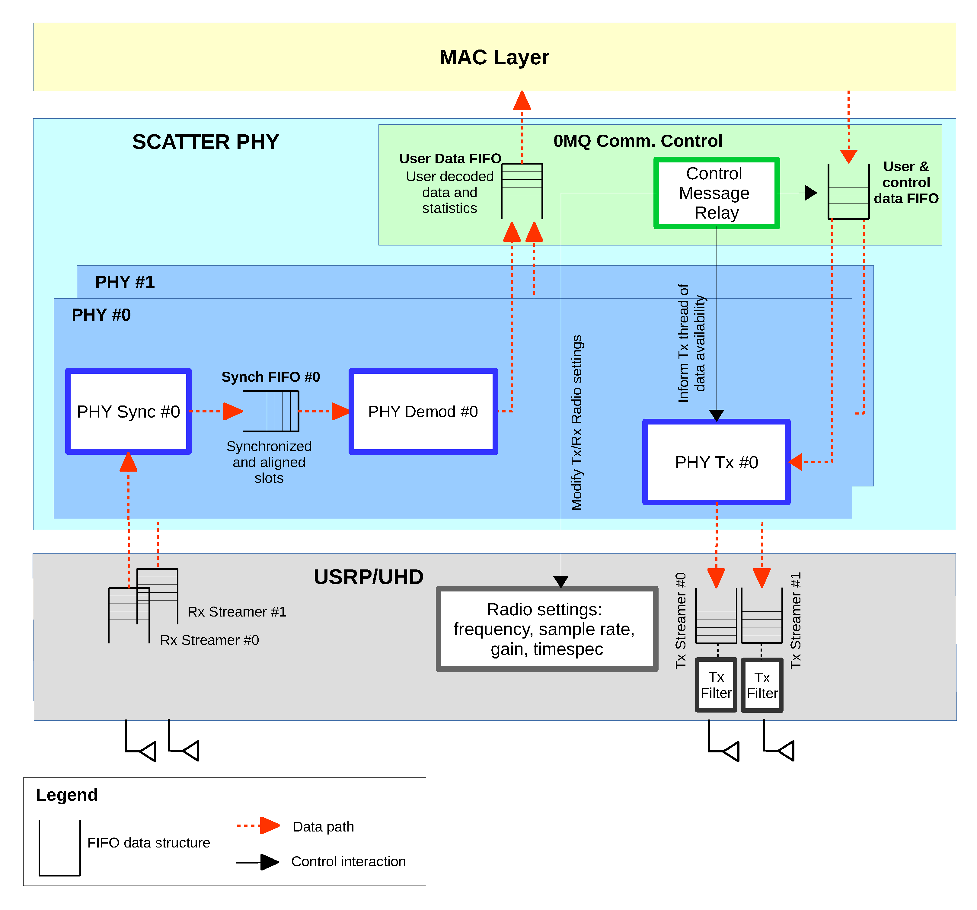
Figure 1 depicts the architecture of SCATTER PHY at a high level. The figure shows the several hardware and software layers making up SCATTER PHY and the different threads running inside of them.
Black arrows indicate the exchange of control and/or information between the threads, while red dashed arrows indicate data paths. SCATTER PHY is a bursty based PHY that transmits data bursts in short intervals. Each bursty transmission interval contains at least one or several transport units, which we call subframes. A subframe is a container through which control and user data are exchanged, over the air, in the network. Therefore, a subframe is the basic transmission unit of SCATTER PHY, and each one is 1 ms long.
The SCATTER PHY is an open-source software defined physical layer [7]. Its implementation makes use of the Universal Software Radio Peripheral (USRP) Hardware Driver (UHD) software Application Programming Interface (API) [6,13], which makes it possible for the PHY to run on top of several Ettus SDR devices such as the Ettus USRP X family of SDRs and National Instruments’ (NI) RIO devices [14,15]. SCATTER PHY accesses the SDR device through the UHD driver and its APIs [16]. As can be seen in the figure, the independent PHY layers are connected to a module responsible for managing the exchange of data, control, and statistics messages with the MAC layer, and the module is known as the ZeroMQ Data/Control Communications module. The exchange messages with the MAC layer are performed through a ZeroMQ bus, also known as 0MQ [5].
In order to establish communications independently with the MAC layer, i.e., decouple the implementation of both layers, a well defined interface (i.e., a set of pre-defined messages) was designed with Google’s Protocol Buffers (protobuf) [17]. Protobuf was used for data serialization and worked perfectly with the 0MQ messaging library [5]. Together, protobuf and 0MQ created a means for a distributed and decoupled exchange of control, statistics, and data messages between SCATTER PHY and MAC layers. SCATTER PHY provides the MAC layer with the ability of real-time configuration of all its parameters and reading of several statistics it measures through the implementation of the 0MQ push-pull message-exchanging pattern [5]. The implementation of this message-exchanging pattern provides upper layers with the ability of locally to configure/read PHY parameters/statistics remotely, i.e., upper layers (e.g., MAC layer) do not need to be run on the same physical radio. The 0MQ push-pull pattern allows MAC and PHY to implement a non-blocking message communications paradigm, i.e., MAC and PHY can exchange data and control messages without having their processing blocked for long periods, and with this paradigm, each layer decides when to check the availability of a new message. The implementation of the 0MQ push-pull pattern and the adoption of the protobuf message library allow SCATTER PHY to be designed and implemented totally independently and decoupled from the MAC layer, i.e., SCATTER PHY’s implementation decisions do not impose any kind of constraints on the programming language, software, or hardware employed by the MAC layer.
SCATTER PHY presents the following set of main features:
  • Bursty transmissions: Short periods of activity (i.e., discontinuous transmissions) allow a better/improved usage of the available spectrum bandwidths. It makes it possible for the radios/networks to coordinate the spectrum access/usage among them in a collaborative, intelligent, or even opportunistic manner.
  • Dual-concurrent PHYs: A Multi-Concurrent-Frequency Time-Division Multiple Access (McF-TDMA) scheme can be implemented by the MAC layer by having two PHYs simultaneously transmitting and receiving at independent frequencies. This ability for concurrent allocations allows for a smarter spectrum utilization as vacant disjoint frequency chunks can be concurrently used.
  • FPGA based filtered transmissions: Filtering the transmitted signal effectively minimizes OOBE, which allows for a better spectrum utilization, once radios can have their transmissions nearer to each other in the frequency domain, helping to mitigate the wastage of spectrum bands.
  • Out-of-band full-duplex operation: Both PHYs operate totally independently of each other, meaning that Tx and Rx modules are able to transmit and receive at different channels, set different Tx and Rx gains, and use different PHY BWs.
  • Timed-commands: This feature allows the configuration in advance of the exact time to (i) start a transmission and (ii) change Tx/Rx frequencies/gains. This allows the MAC layer to implement a TDMA scheme.
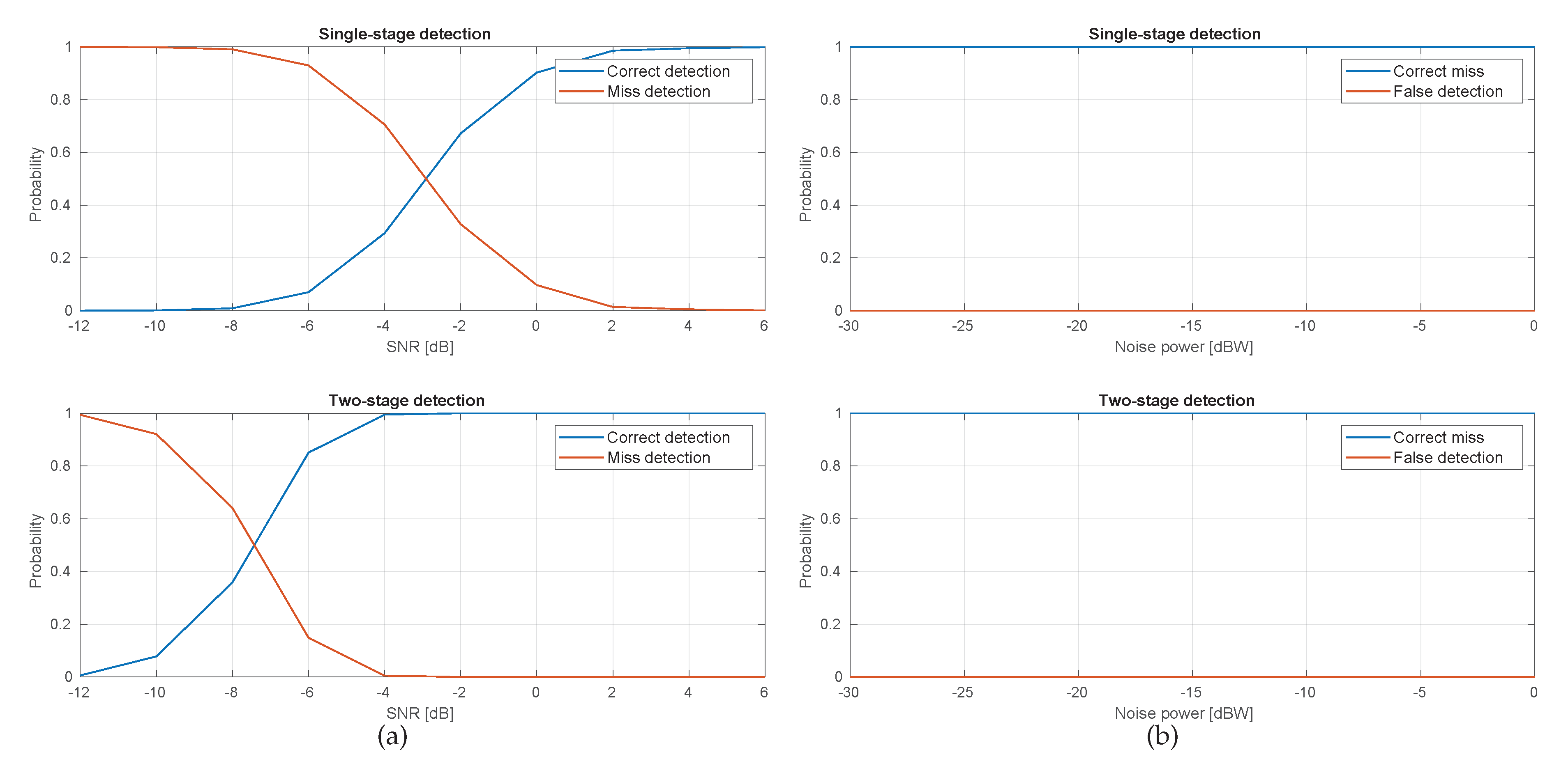
  • Improved synchronization: Through the design and implementation of a novel two-stage synchronization algorithm, it is possible to improve the packet detection ratio when compared to the single-stage approach.
  • Fine-grained CP based CFO estimation: By generating a complex exponential sequence with smaller sampling steps, it is possible to synthesize the frequency offset more accurately, consequently improving the correction.
  • Channel emulator: Through the implementation of an abstraction layer between the USRP hardware and the software based PHY, it is possible to create a channel emulator that connects the transmission side to the receiving side without the necessity of any hardware. Through the use of the channel emulator, it is possible to test novel PHY layer algorithms with the addition of white Gaussian noise, multi-paths, frequency offsets, etc.
SCATTER PHY was implemented based on the srsLTE library [18]. srsLTE is an open-source and free LTE software based library that was developed by the Software Radio Systems (SRS) Limited company [18]. It implements LTE release 10 and a few narrow-band Internet-of-Things (IoT) and 5G features. As SCATTER PHY was built on an LTE-like library, it consequently absorbed and evolved on top of the existing 4/5G features.
We employed OFDM as the SCATTER PHY waveform. OFDM is a full blown technology that is present in a huge number of commercial products due to various advantages it offers such as low implementation complexity, robustness to severe multi-path fading, simple channel estimation, easy integration with Multiple-Input Multiple-Output (MIMO) technology, etc. [19]. User and control data are mapped into subcarriers over 14 OFDM symbols spanning 1 ms. The control data signal carries the used MCS for the current transmission and the number of subsequent subframes with user data modulated with that specific MCS.
The control data signal is used by the independent PHY receivers to detect the number of allocated RBs automatically (i.e., control is embedded into the transmitted data signal), the MCS value selected to transmit data of a specific device/radio, and the location of the allocated RBs in the subframe’s resource grid.
By embedding the control information into the transmitted signal, the Medium Access Control (MAC) layer does not need to know in advance the number of subframes and MCS in a given Channel Occupancy Time (COT). After successful user data decoding, each one of the PHYs independently notifies the MAC layer about the corresponding decoded MCS value, the number of received data bytes, and decoding statistics (e.g., RSSI, SINR, number of detection/decoding errors, etc.).
SCATTER PHY works with two types of subframes, namely synchronization and data-only subframes. A synchronization subframe carries the synchronization signal, reference signal, control, and user data. A data-only subframe carries the reference signal and user data. The synchronization signal is a 72 symbol long sequence that is generated using Zadoff–Chu (ZC) sequences [20,21]. Therefore, the synchronization sequence is generated according to:
x s = e j π u n ( n + 1 ) N Synch , 0 n N Synch 1 ,
where n is the sequence sample index, u is the ZC sequence index, and N Synch is the length of the synchronization sequence.
The control signal is based on Maximum length sequences (M-sequences) [22], where two M-sequences, each of length 31, are used to transmit the information necessary to decode the user data. The reference signal is used to estimate the channel and then equalize the received signal so that channel interference to the desired signal is minimized.
The SCATTER PHY allows bursty transmissions with a variable Channel Occupancy Time (COT), i.e., the number of subframes to be transmitted in a row without any idle time (i.e., gap) among consecutive subframes is variable and depends on how many bytes the MAC layer has to transmit. The number of subframes in a COT is calculated based on the number of data bits to be transmitted, PHY BW, and MCS parameters forwarded by the MAC layer to each PHY layer in the control messages. The smallest COT value is equal to 1 ms and corresponds to the transmission of a synchronization subframe. Having a variable COT allows SCATTER PHY to support various types of traffic loads. Every subframe carries a pre-defined number of bytes. The number of bytes is calculated based on the subframe type, selected MCS, and configured PHY BW.
As can be seen in Figure 1, each one of the PHY modules is divided into three sub-modules, namely PHY Rx synchronization, PHY Rx demodulation, and PHY Tx. Each one of the sub-modules runs on a standalone and exclusive thread. A multi-threaded PHY implementation allows independent, time-consuming, and critical processing tasks to be executed concurrently (i.e., simultaneously), improving efficiency and computing performance. In combination with multi-core enabled CPUs, the multi-threaded PHY modules straightforwardly support communications in full-duplex mode, i.e., each individual and independent PHY is able to receive and transmit simultaneously at different frequencies. The direct consequence of the full-duplex mode is that it results in higher throughput. Each PHY Tx thread ( # 0 and # 1 
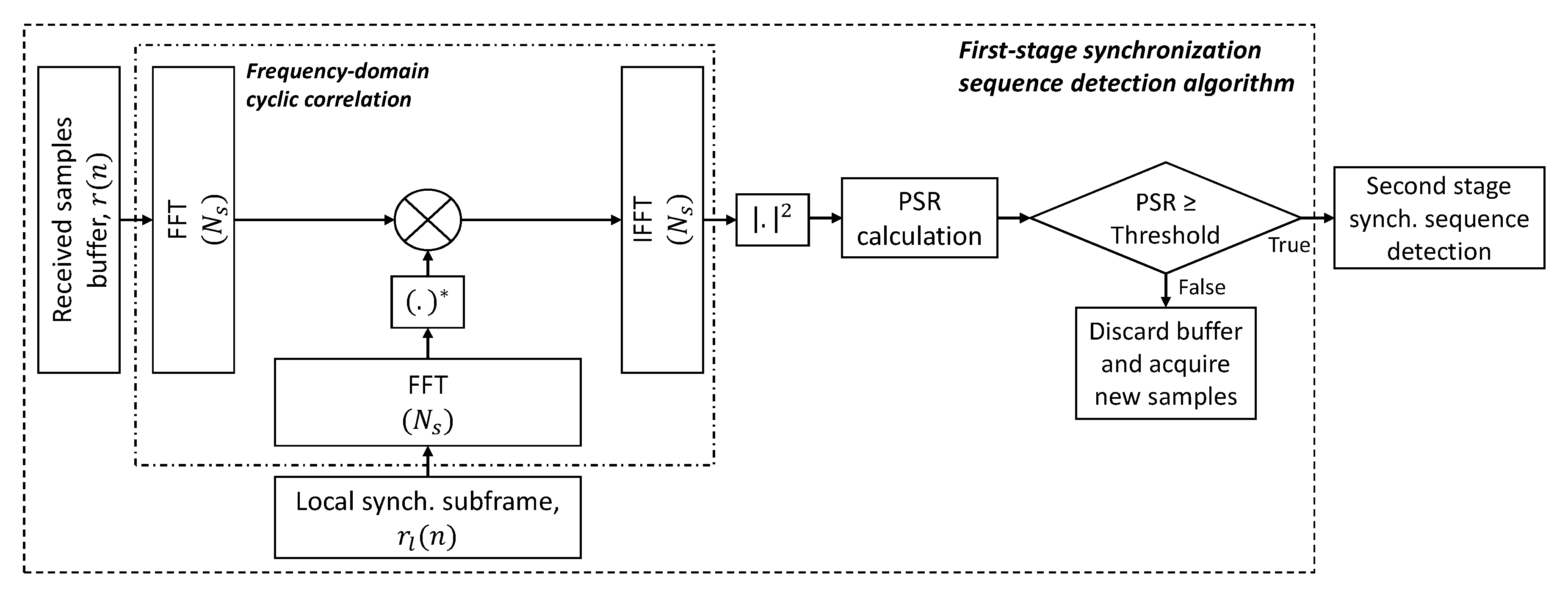
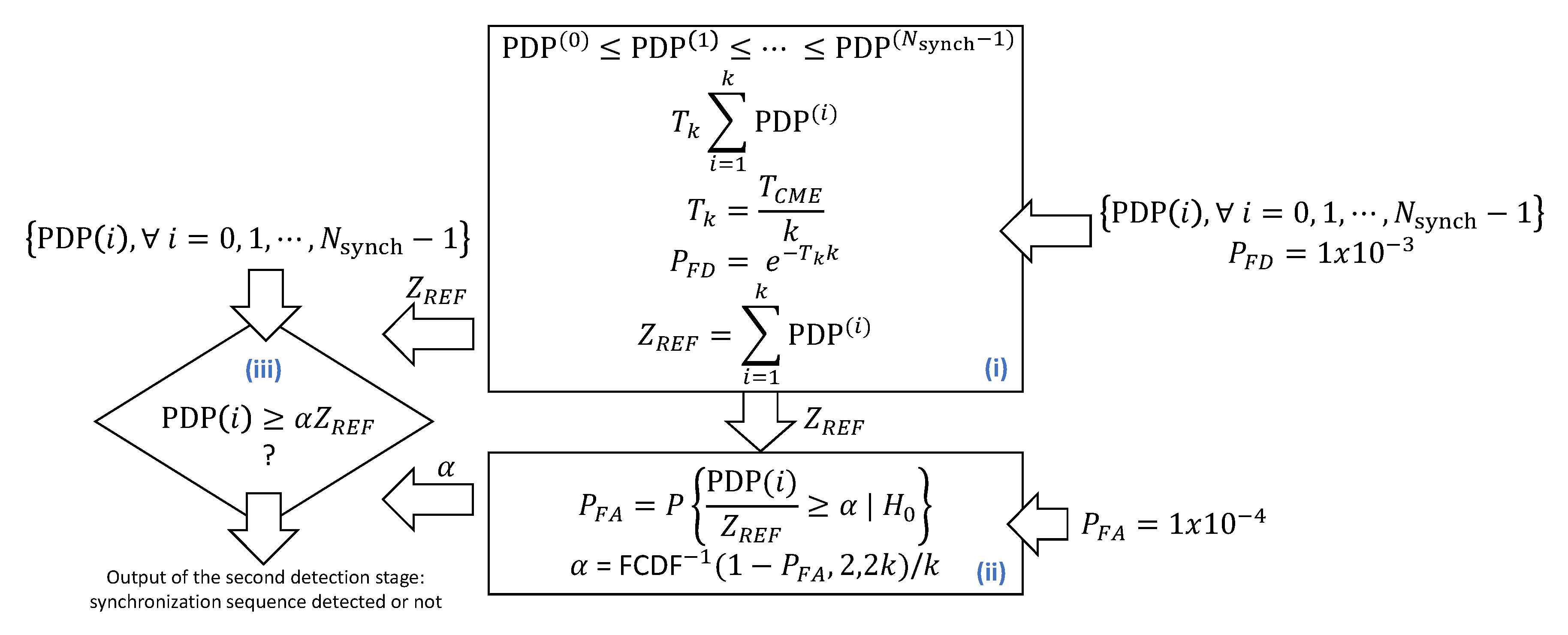
) is responsible for modulating and transmitting data (i.e., control and user data). On the other hand, each PHY Rx synchronization thread is responsible for detecting the Synchronization (Synch) sequence, decoding the control data, frequency offset estimation/correction, and time-alignment of the detected subframes. Detection of the Synch signal is carried out through a two-stage detection algorithm, which at the first stage correlates the received signal with a locally stored version of the synchronization subframe with no data and control signals. If the Peak-to-Side-lobe Ratio (PSR) is greater than a constant threshold, then the second stage applies a CA-CFAR algorithm to the OFDM symbol carrying the Synch signal [20]. The two-stage approach employed by SCATTER PHY improves the Synch signal detection when compared to a detection approach that only uses the PSR of the correlation calculated at the first stage. The two-stage approach employed by SCATTER PHY is described in Appendix A.
The CFO estimation task is split into coarse and fine estimations/corrections, where the coarse estimation is based on the Synch signal and the fine estimation is based on the Cyclic Prefix (CP) portion of the OFDM symbols [23]. The integer part of the frequency offset (i.e., integer multiples of the subcarrier spacing) is estimated and corrected by the coarse CFO algorithm, which is based on the maximization of the correlation of the received synchronization signal with several locally generated frequency offset versions of it. On the other hand, the fractional frequency offset (i.e., offset values less than one half of the subcarrier spacing) is estimated and corrected by the fine CFO algorithm, which is based on the phase difference of the correlation between the CP and the last part of the OFDM symbol (i.e., the portion used to create the CP). Integer and fractional CFO estimation methods are described in Appendix B.
Each PHY Rx demodulation thread is responsible for OFDM demodulation (CP removal and FFT processing), i.e., user data demodulation, channel estimation/equalization, resource de-mapping, symbol demodulation, de-scrambling, de-interleaving/de-rate matching, turbo decoding, de-segmentation, and finally, cyclic redundancy check (CRC) checking. Each one of the independent PHYs receives control and data messages from the 0MQ Communications Data/Control module. Decoded user data and Tx/Rx statistics are sent directly to the MAC layer through the 0MQ bus within a protobuf pre-defined message. 
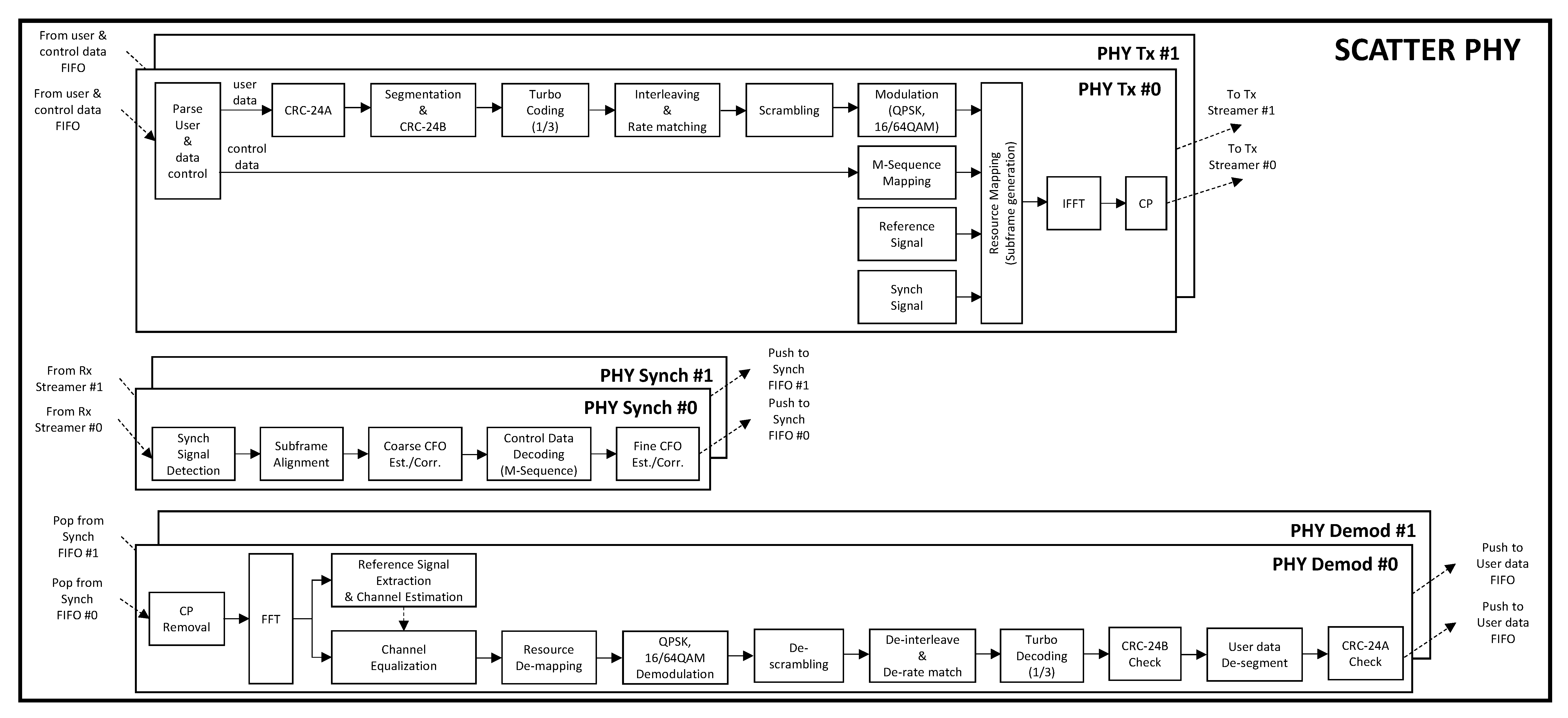
Figure 2 presents the block-diagram of SCATTER PHY. It shows the blocks making up the receiver (PHY Synch and PHY Demodulation (Demod) threads) and transmitter (PHY Tx thread) sides of each independent PHY.
When it comes to numerology, SCATTER PHY adopts a subcarrier spacing of 15 kHz, a CP of 5.2 μ s, and supports 1.26 , 2.7 , 4.5 , and 9 MHz bandwidths, which are equivalent to the LTE bandwidths of 6, 15, 25, and 50 resource blocks, respectively [19]. Each one of the PHY’s transmission channel Bandwidth (BW) can be configured in real time, through the Tx control messages or via command line at the system’s startup. The OFDM modulation parameters adopted by SCATTER PHY are summarized in Table 1.
The only difference between the OFDM modulation parameters listed in Table 1 and the LTE ones [19] is the FFT size and, consequently, the resulting sampling rate for the PHY BWs of 4.5 and 9 MHz. The reason for employing these non-standard sampling rates is to reduce the computational load of SCATTER PHY and to reduce the data transfer rate required to move base-band IQ (i.e., In-phase/Quadrature) samples between the RF front-end (i.e., the USRP device) and the base-band processor (i.e., the host PC) and vice versa. For example, for a PHY BW of 4.5 MHz, the standard LTE sampling rate would be equal to 512 FFT points × a subcarrier spacing of 15 kHz = 7.68 MHz. However, out of the 512 subcarriers, only 300 are useful subcarriers, where the remaining ones are left unused as guard-band subcarriers. Therefore, by employing a smaller FFT size and, consequently, a lower sampling rate, while keeping the same subcarrier spacing, SCATTER PHY can still successfully demodulate all occupied subcarriers. Therefore, the computational load is lower due to the fact that fewer base-band samples have to be moved between the USRP and the host PC.
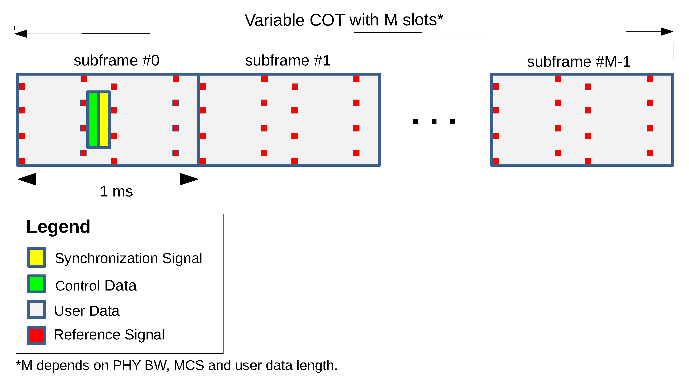
The frame structure employed by SCATTER PHY is presented in Figure 3. As can be seen, signals regarding synchronization and control data are only added to the first subframe of a COT, while the subsequent subframes carry only reference signals and data symbols. With this frame structure, synchronization (i.e., detection of synchronization signal, time-alignment, and CFO estimation/correction) and control data decoding only happen for Subframe # 0 , i.e., the synchronization subframe. The differences between the proposed frame structure and LTE’s are (i) no modulated control data (i.e., LTE’s PDCCH channel) being added to first OFDM symbols, (ii) a longer synchronization signal, which improves the subframe detection performance, (iii) control data sent via M-sequences, which makes the control data decoding more robust against interference and noise, and (iv) no division of the subcarriers into resource blocks, once all subcarriers are allocated to a single user only. As shown in Figure 3, and differently from LTE, SCATTER PHY’s frame structure does not carry control data in the first OFDM symbols, which, consequently, gives more room, i.e., subcarriers, for user data transmission. Therefore, it is possible to achieve higher throughput when compared to the LTE standard.
The Payload Data Unit (PDU) employed by SCATTER PHY is known as the Transport Block (TB). A TB is the container carrying data that are created at the MAC layer and transferred to the individual PHYs to be encoded and transmitted. One TB is composed of a number of bytes that can be accommodated inside a 1 ms long subframe, given the configured MCS and PHY BW parameters. Therefore, given the PHY BW and the desired MCS, the MAC layer can calculate the number of bytes that can be handled by a 1 ms long subframe. Table 2 presents the coding rate for each one of the 32 defined MCS values.
The differences between SCATTER PHY’s modulation code scheme and LTE’s are (i) 32 different MCS values instead of the 29 defined in the LTE standard, where the three additional MCS values allow SCATTER PHY to reach higher data rates in high SNR scenarios, and (ii) the greater number of subcarriers per subframe, which are used for user data transmission and, consequently, increase the final achieved throughput. However, even though being able to carry more user data per subframe, we kept the same coding rate of the LTE standard for MCS values ranging from zero to 28.
Communications between SCATTER PHY and the MAC layer are performed through four pre-defined (i.e., protobuf) messages. The first two messages, named Rx and Tx control, are employed, as the name suggests, to control/configure subframe reception and transmission, respectively. The parameters transported by these two control messages are set and sent to the individual PHYs by the MAC layer before the transmission of every new COT, hence allowing on-line parameter configuration. The other two messages, named Rx and Tx statistics messages, are employed to provide the MAC layer with real-time feedback from each independent PHY, providing critical information that is necessary for such a layer to take important actions.
Tx control messages transport the TBs (i.e., user data) to be transmitted and Tx parameters regarding that transmission, that is PHY ID, Tx gain, Tx channel, data length, MCS, Tx PHY BW, and transmission timestamp. The transmission timestamp parameter allows time scheduled transmissions, which consequently enable the MAC layer to implement a Multi-Frequency (MF) Time Division Multiple Access (TDMA) medium access scheme. Rx control messages are employed to configure Rx gain, the Rx channel, the maximum number of turbo decoder iterations, enable or disable Rx combining, and Rx PHY BW of a specific PHY, addressed through the PHY ID parameter. The PHY ID parameter is used to specify for each one of the two PHYs a control message.
Tx statistics messages inform the MAC layer about transmission statistics like data coding-time and the total number of transmitted subframes of each independent PHY. Rx statistics messages transport the received data, PHY ID, and reception statistics regarding the received data such as Received Signal Strength Indication (RSSI), Channel Quality Indicator (CQI), decoded MCS, decoding time, subframe error counter, number of turbo decoder iterations, etc. The real-time configurable parameters and statistics offered by SCATTER PHY are summarized in Table 3.

3.1. COT-Based Filtering

Due to their poor spectral localization, OFDM based wave-forms are not suited for spectral coexistence [24]. This issue is due to the rectangular pulse-shape intrinsically employed by the OFDM wave-form, which leads, in the frequency domain, to a sync-pulse property with a very low second-lobe attenuation of approximately 13 dB [25].
Therefore, in order to guarantee lower OOBE, i.e., improved spectral-localization, and still maintain the orthogonality of the OFDM symbols, it is necessary to filter the generated subframes before their transmission [6]. The filtering process is applied to each COT of each PHY independently. The subframes comprising a COT are generated at the SW level and then filtered at the HW level, by a 128 order FPGA based FIR filter. The COT based filtering improves the closer coexistence with other radios (either belonging to our team or others), allowing radio transmissions to be closer in frequency. The filter used in SCATTER PHY was designed and explained in [6].
This co-design SW/HW is used so that fast processing high order filters can be implemented adding up very low latency to the transmission chain and still allowing the flexibility of the software defined PHYs.
The coefficients of the filters applied to the COT are automatically selected in real time based on the Tx PHY BW parameter carried by the Tx control message. The coefficients are automatically chosen as the filters’ cut-off frequencies have to match and exactly filter the desired signal’s bandwidth, i.e., the configured PHY transmit BW.
The normalized FIR filter’s coefficients used in the COT based filtering are given in time domain by [6]:
f ( n ) = p ( n ) w ( n ) k p ( k ) w ( k ) .
where p ( n ) is the impulse response of the sincsignal and w ( n ) is the window used to truncate the sinc signal. These two signals are given as:
p ( n ) = sin π [ N U + N e ] n N FFT / π [ N U + N e ] n N FFT , n 0 , 1 , n = 0 .
w ( n ) = 1 2 1 + cos 2 π n L 1 0.6 ,
where N U is the number of useful subcarriers (see Table 1), N FFT is the length of the FFT used in the OFDM modulation (see Table 1), N e is the excess bandwidth in the number of subcarriers, L is the length of the FIR filter, and ( L 1 ) 2 n ( L 1 ) 2 . The excess bandwidth is used to extend the flat region of the filter so that the subcarriers at the left and right borders of the OFDM symbols suffer less attenuation.
The filter, f ( n ) , exhibits the following properties: (i) a time duration that is comparable to a small fraction of an OFDM symbol’s duration, (ii) a sharp transition-band, which minimizes the necessary guard-bands, (iii) a flat pass-band over the useful subcarriers, and (iv) fair stop-band attenuation [6].

3.2. Benefits of SCATTER PHY

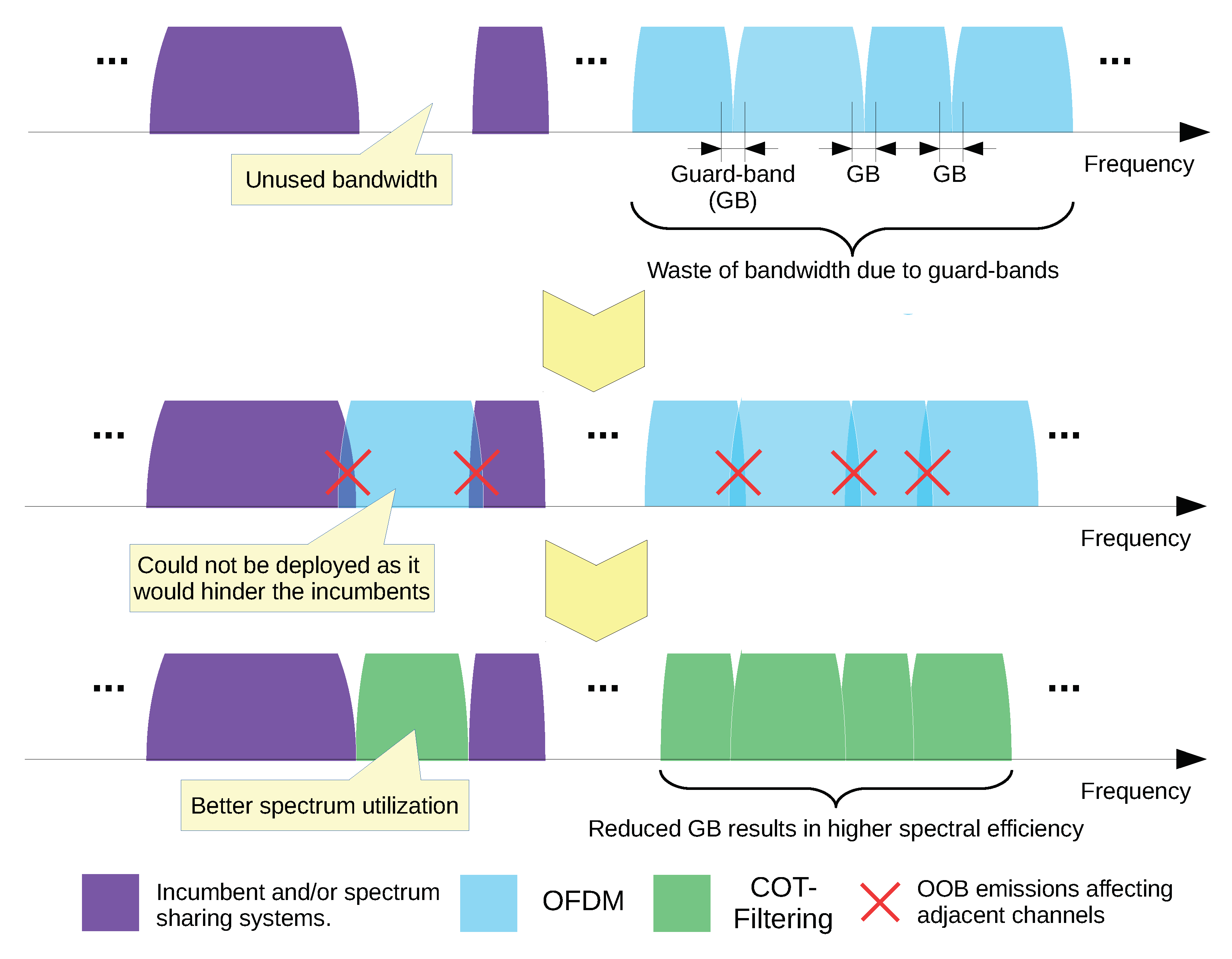
In this section, we describe the two main advantages of SCATTER PHY. The first advantage is that the COT based filtering mitigates OOBE, making SCATTER PHY more spectrally efficient. OOBE might interfere with radios using adjacent channels, decreasing the quality of the signals received by them. Therefore, the interference caused by OOBE impacts directly on the throughput achieved by those radios. The reduced OOBE allows SCATTER PHY to operate closer, in the frequency domain, to radios transmitting at adjacent channels. This, in turn, reduces spectrum band wastage by increasing the spectral efficiency, as depicted in Figure 4. The second advantage offered by SCATTER PHY is that it is possible to configure all PHY parameters in real time through the control messages. This makes SCATTER PHY a very flexible and agile SDR based PHY, allowing higher layers to configure the available parameters based on spectrum band availability, for instance.

4. Experiment Results

In this section, we demonstrate the effectiveness and usability of SCATTER PHY by presenting the results of several experiments. The experiments were executed with SCATTER PHY running on servers equipped with Intel Xeon E5-2650 v4 CPUs (@ 2.2 GHz, 30 M cache, 9.60 GT/s QPI, turbo, HT, 12 cores/ 24 threads, 105 Watts), 128 GB of RAM memory connected to x310 USRPs with 10 Gigabit Ethernet links, and equipped with CBX-120 RF daughter-boards [26].
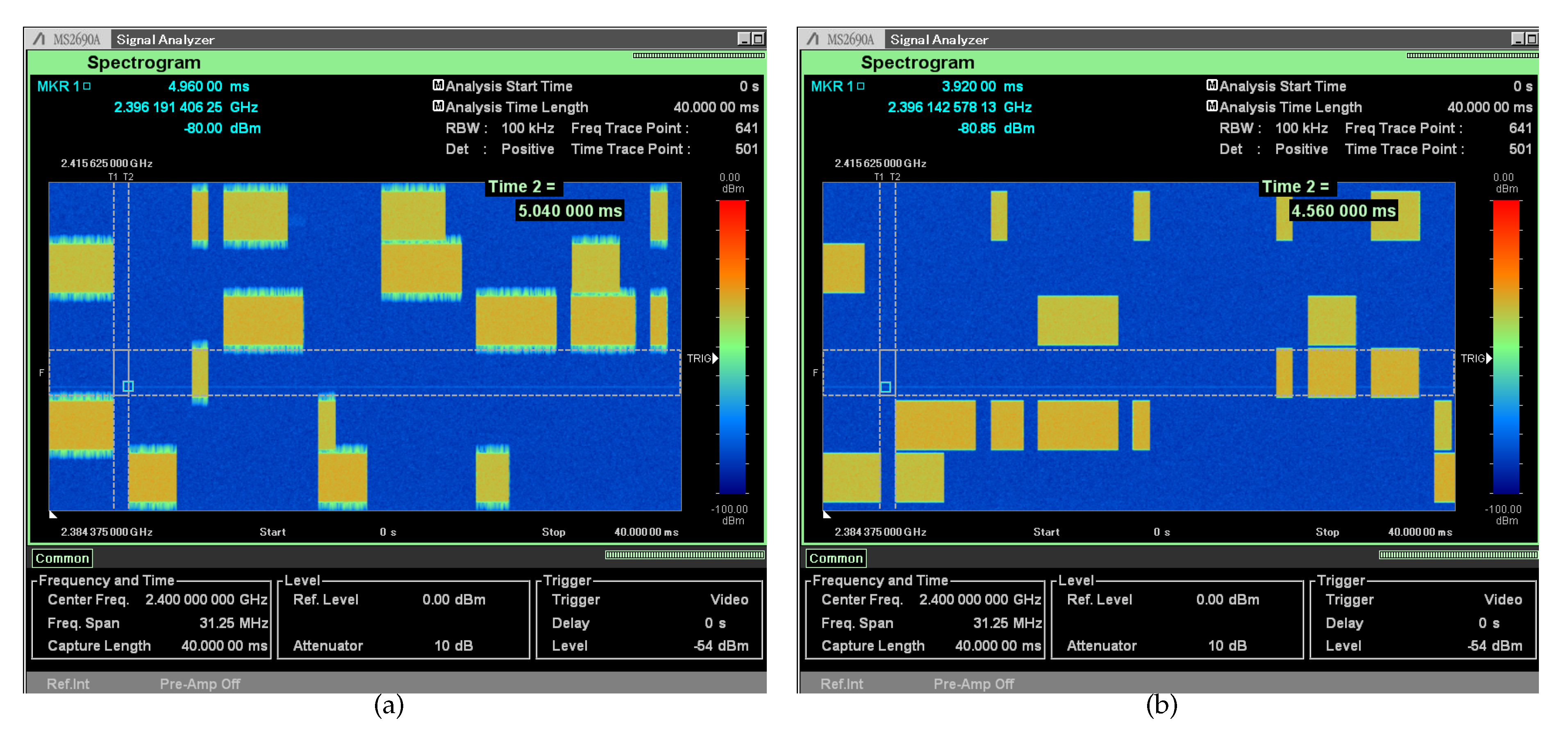
Figure 5 depicts two spectrograms (i.e., the visual representation of the spectrum of frequencies of a signal as it varies over time) saved for 40 ms over a 31.25 MHz bandwidth with both PHYs set to operate concurrently, at each instant, at two of six 4.5 MHz channels. This experiment intends to show that SCATTER PHY is able to generate two concurrent and independent transmit channels per node. For this experiment, each PHY transmits at randomly selected channels a random number of subframes. The number of transmitted subframes, i.e., COT, and the channel number are randomly selected between the ranges of 1–3 and 0–5, respectively. Here, a gap of 1 ms between consecutive transmission is used. The figures were saved with the center frequency of both Tx PHYs set to 2.4 GHz, equal Tx gains of 3 dB, and both USRP Tx outputs connected to the signal-analyzer via an RF combiner and a coaxial cable presenting a 20 dB attenuation. As can be seen in both figures, Figure 5a,b, SCATTER PHY was able to independently transmit at two distinct channels with a different number of subframes. Figure 5a shows the case where no filtering was enabled. As can be noticed, OOBE might cause interference to radios operating at adjacent channels and consequently decrease their throughput. Figure 5b shows the case when the FPGA based FIR filters were enabled. As can be noticed, when filtering was enabled, OOBE was mitigated. Therefore, by enabling filtering, the interference that could be impacting radios operating at adjacent channels was mitigated. Moreover, another direct consequence of using filters was that the channel spacing, i.e., the guard-band between adjacent channels, could be decreased, decreasing the wastage of spectrum band, consequently.
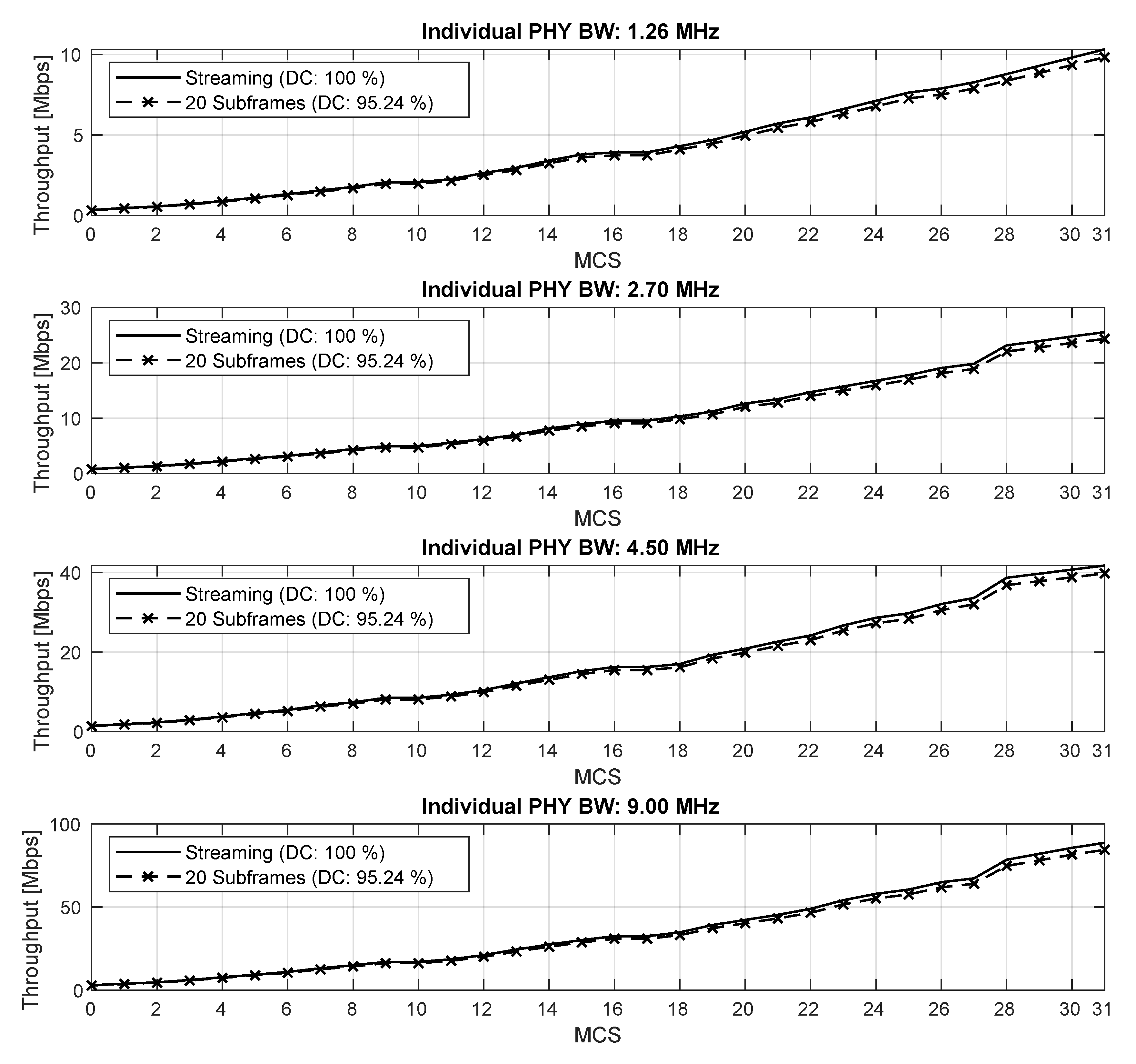
Figure 6 shows measurements of the throughput, which were taken with SCATTER PHY working in full-duplex mode, where the two independent PHYs simultaneously and concurrently receive and transmit, for several MCS and PHY BW values. The full-duplex mode was used so that we could check if it somehow impacted the throughput measurements, once, in this mode, SCATTER PHY was fully utilized. The throughput measurements were taken for COTs of 20 ms with gaps of 1 ms between subsequent COT transmissions, which resulted in a Duty-Cycle (DC) of 95.24%. The final throughput was calculated as the average over 10 throughput measurement intervals of 10 seconds each. For each measurement interval, the number of bits received during that interval was counted and then divided by the length of the interval, resulting in a throughput measurement. This procedure was repeated 10 times, and then, the individual measurements were averaged. The SNR on the link was set to 30 dB so that the packet reception rate for all MCS values was equal to one. For the sake of comparison, we added to the figure the theoretical maximum throughput achieved when a DC of 100% was used; we called it streaming mode, due to the fact that there was no gap between subsequent subframes. The theoretical maximum throughput was obtained by dividing the size of the TB, given in number of bits for each MCS value, by the subframe time interval, i.e., 1 ms. As expected, the throughput measured with SCATTER PHY was close to that of the streaming mode for all PHY BW and MCS values, achieving more than 84 Mbps for MCS 31 and a PHY BW of 9 MHz. Moreover, full-duplex mode operation had no visible impact on SCATTER PHY’s achieved throughput. This result comes from the fact that SCATTER PHY ran on a powerful server, with 12 cores and 128 GB of RAM memory.
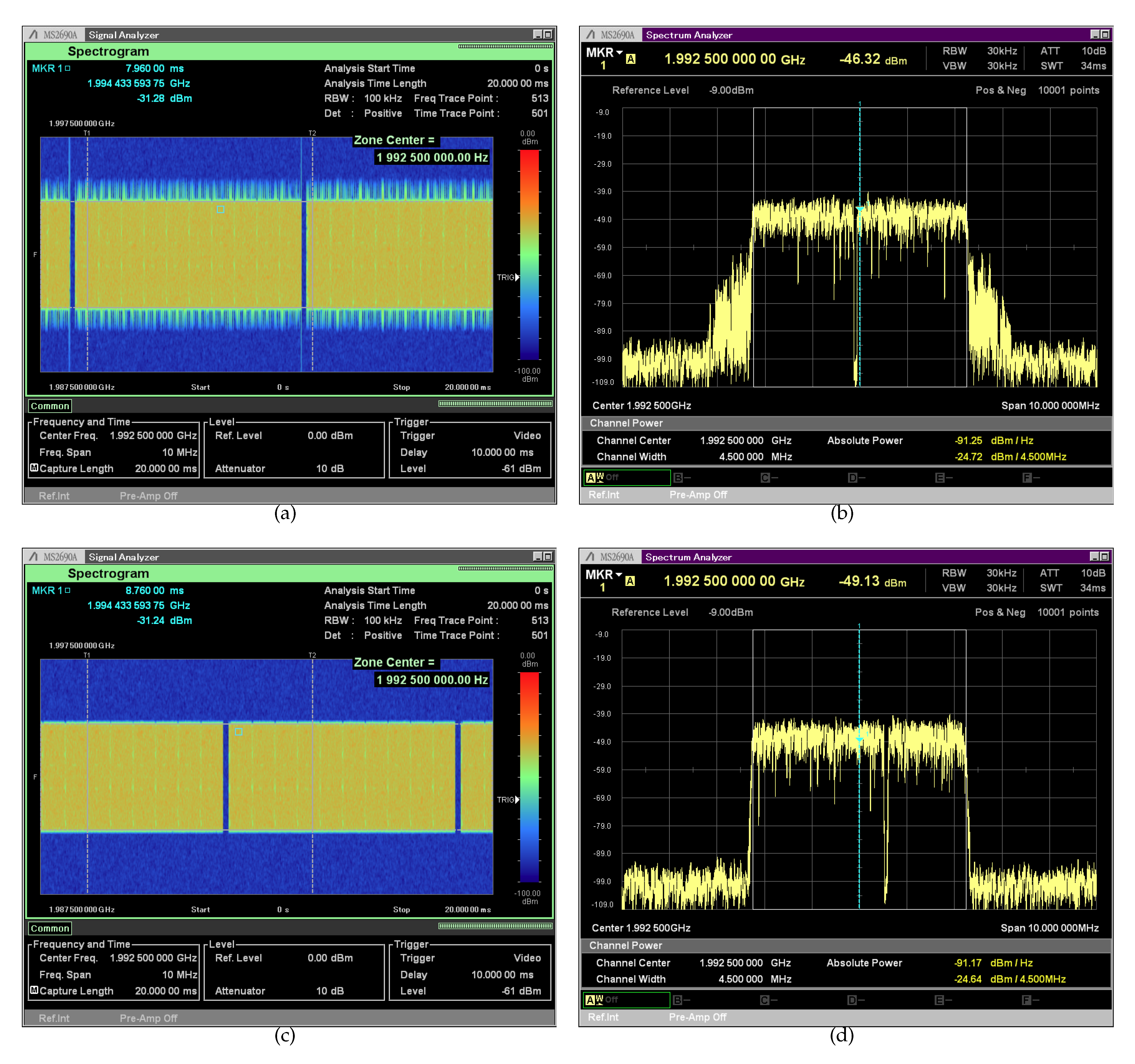
Figure 7 depicts the comparison of the spectrogram and spectrum of filtered versus unfiltered transmissions. SCATTER PHY was able to enable or disable the FPGA based transmission filters at the command line. These results were saved with an Anritsu MS2690A Signal Analyzer. In the experiment, the signal analyzer sat beside the USRP hardware. The shown results were saved with SCATTER PHY’s Tx gain set to 3 dB (this was configured through the control messages), Tx center frequency set to 1.9925 GHz (this was configured through at command line at start-up), and with the USRP’s Tx output connected to the signal analyzer via a coaxial-cable connected to an attenuator with 20 dB of attenuation. As can be seen, OOBE (i.e., the OFDM lateral skirts) were mitigated when the 128 order FPGA based FIR filters were enabled. The results show the transmission of only one of two PHYs, the outcome being the same for the other PHY.
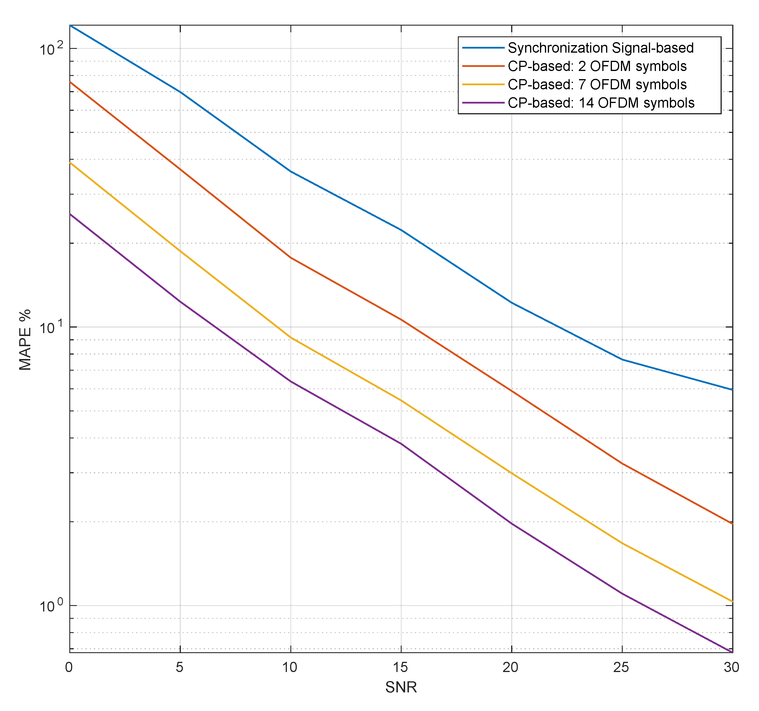
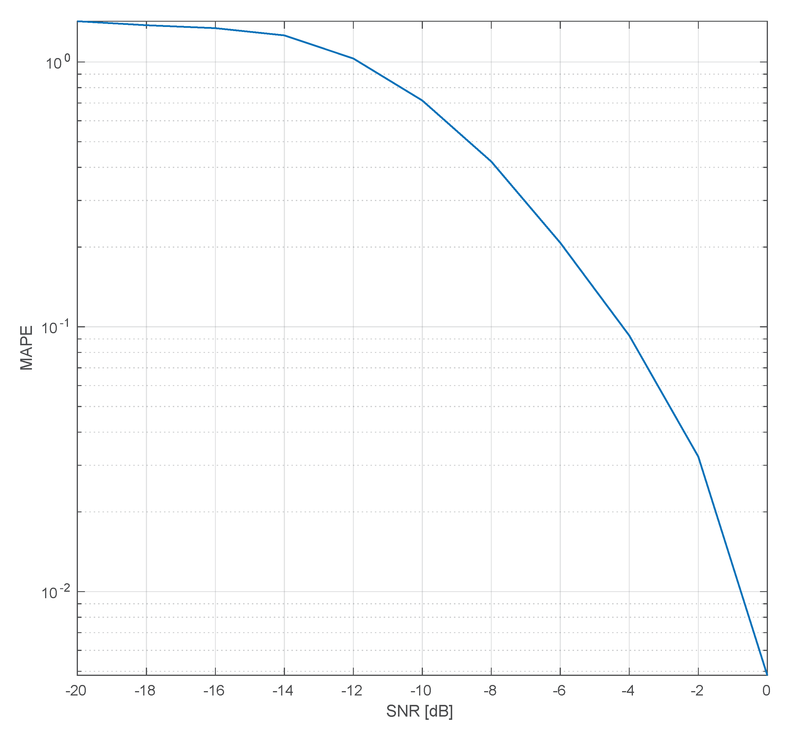
Figure 8 compares the Mean Absolute Percentage Error (MAPE) of the fine CP based fractional CFO estimation method against fractional CFO estimation based on the synchronization signal. The MAPE for the CFO estimation is defined as:
MAPE % = 100 N i = 1 N | CFO est . ( i ) CFO ( i ) CFO ( i ) | ,
where CFO est . ( i ) is the estimated CFO value for the i th trial, CFO ( i ) is the randomly generated CFO, which is applied to the transmitted signal, for the i th trial, and N is the number of trials over which the CFO is averaged. The results were obtained by connecting the Tx port to the Rx port of the same USRP so that the frequency offset caused by the HW was minimal or nonexistent and adding Additive White Gaussian Noise (AWGN) plus the desired frequency offset at the SW level just before the subframes were transmitted. The CFO applied to the signal was drawn from a uniform distribution varying from 7.5 kHz to + 7.5 kHz, i.e., + / half subcarrier spacing. As can be seen, the fine CFO estimation algorithm, which was based on the CP portion of the OFDM symbols, outperformed the Synch based CFO algorithm even when only two consecutive CPs were averaged. Additionally, we see that the performance of the CP based estimation improved as the number of averaged CPs increased; however, the downside of averaging more CPs was an increase in the processing time. The CP based CFO estimation method employed by SCATTER PHY was an improvement over the CFO estimation implemented by srsLTE. The SCATTER PHY implementation employed Single-Instruction Multiple-Data (SIMD) instructions in order to decrease the CFO estimation and correction computational time, allowing it to use more averaged CPs. Additionally, SCATTER PHY implemented a more accurate and fine-grained complex exponential signal for generating the correction signal, making it possible to generate signals with frequencies that were closer to the estimated ones.
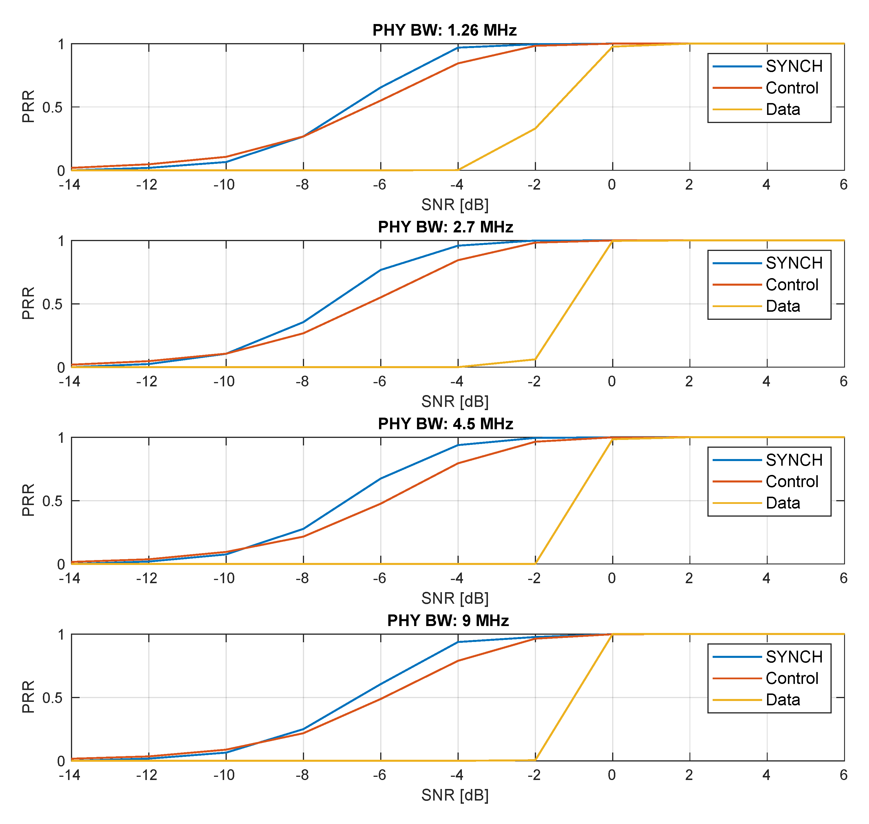
Figure 9 presents the comparison of the Packet Reception Rate (PRR) for each one of the signals carried by a SCATTER PHY subframe, namely synchronization, control, and data signals over several SNR and BW values. The SNR was calculated based on the power of a 1 ms subframe; therefore, before adding noise to the transmitted subframe, the subframe power was calculated, and then, the necessary noisy power to achieve the desired SNR was calculated. The MCS used for modulating the user data was set to zero, which was the most robust coding scheme, allowing SCATTER PHY to decode data in low SNR scenarios. The purpose of this experiment was to identify the lowest possible SNR at which SCATTER PHY could still correctly decode the user data. This experiment was run by adding a channel emulator between the Tx and Rx sides of a single PHY instance. At the Tx side, the generated subframes, instead of being sent to the USRP HW, were sent to an abstraction layer that emulated the HW and added AWGN noise to the transmitted signal. Next, the abstraction layer transferred the noisy signal to the receiving side of the PHY. The PRR was averaged over 10 4 trials, where at each trial, the Tx side of the PHY sent a single synchronization subframe. As can be seen, synchronization and control signals had a better PRR performance than that of the data decoding; however, SCATTER PHY’s PRR performance was limited by the ability to decode correctly the data section of a subframe. Additionally, we see that the data PRR was better for the 1.26 MHz case, which was due to the fact that compared to the other BW values, MCS 0 for the 1.26 MHz case carried more redundancy bits, as shown by Table 2, making it more robust against noise. The other two signals, synchronization and control, presented similar PRR curves for all BW values. Moreover, it is noticeable that the data PRR was equal to 1 for SNR values greater than or equal to 0 dB.
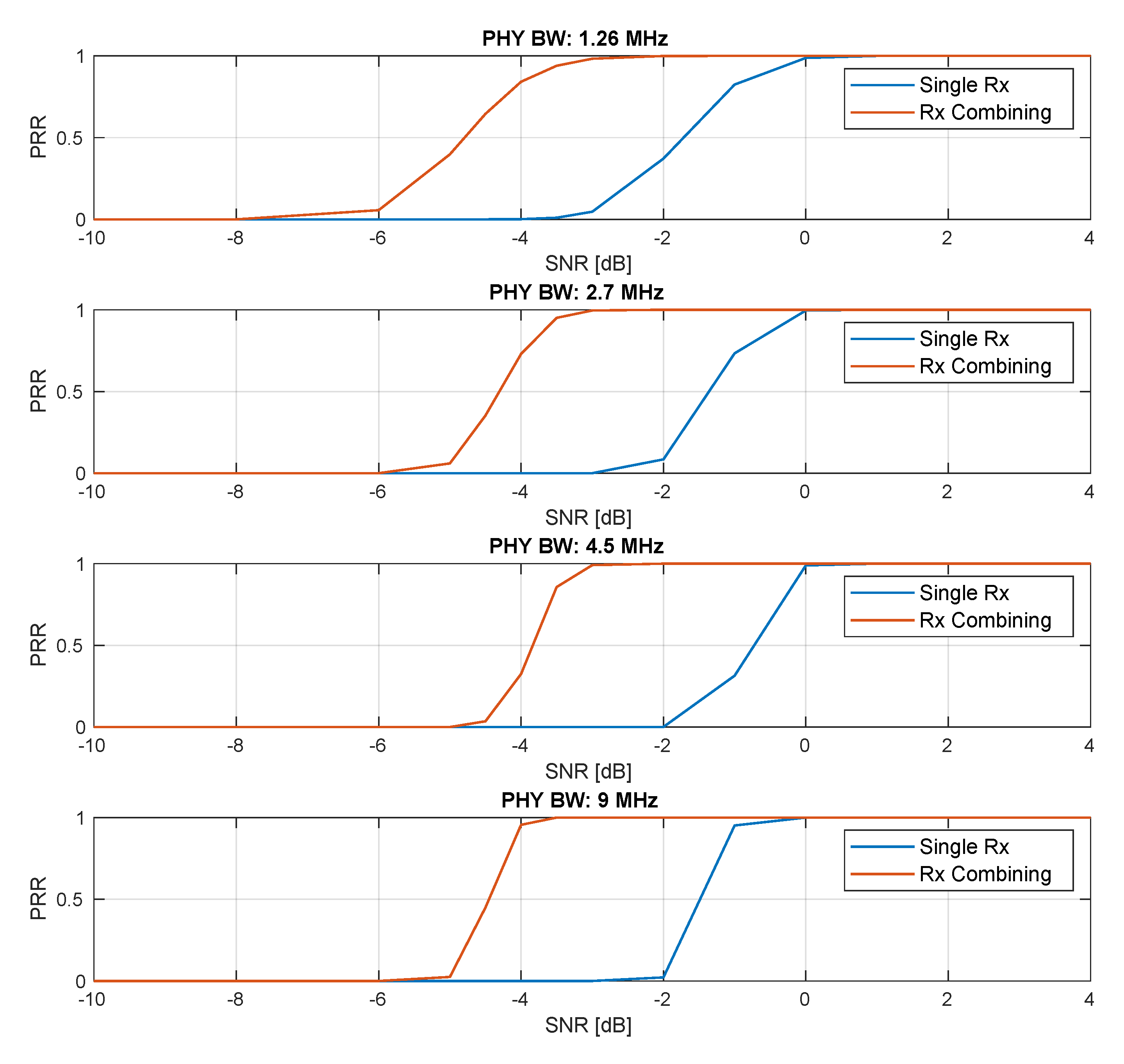
Figure 10 presents the result of the comparison of single Rx data decoding and that of a simple Rx combining scheme that can be implemented with SCATTER PHY. The figure shows data decoding PRR results for both receiving schemes. Here in this case, after synchronization (Synch signal detection, CFO estimation/correction, control data decoding, and subframe alignment), the two independently synchronized subframes were combined through a simple average of both subframes as defined in (6).
r comb . ( n ) = 1 N ant . i = 1 N ant . r Rx i ( n ) ,
where N ant . is the number of Rx antennas (in our case, N ant . = 2 ), r Rx i ( n ) is the subframe synchronized at the i th antenna, and r comb . ( n ) is the resulting combined subframe signal. The MCS value used in this experiment for all PHY BWs was zero. As can be seen, the Rx combining scheme employed in this experiment provided a processing gain ranging from 2.5 to 3 dB over the single Rx approach. With this scheme, SCATTER PHY was able to combine the received subframes for improved performance in low SNR scenarios.
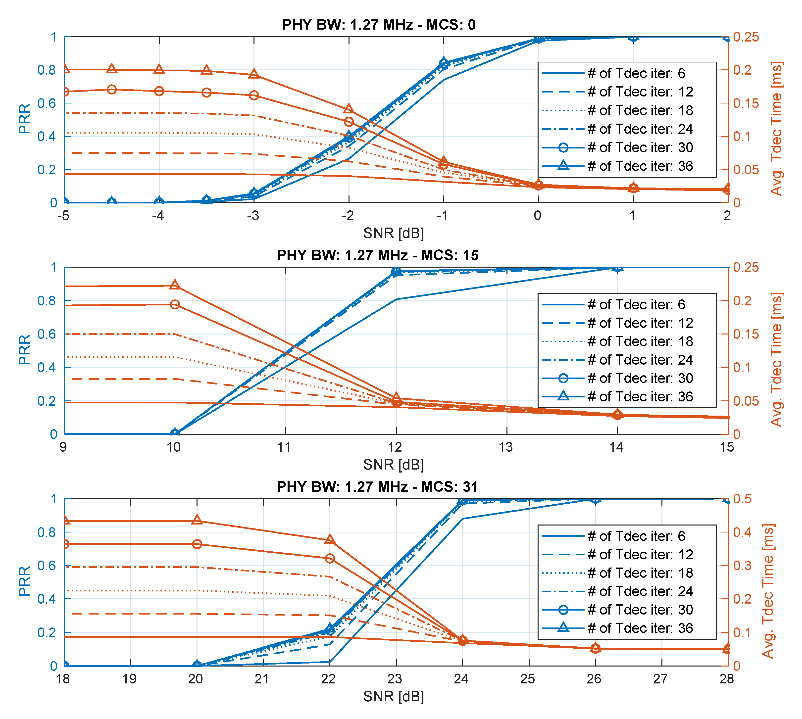
Figure 11 presents the results on the variation of the maximum number of turbo decoding iterations for a PHY Tx BW of 1.27 MHz and three different MCS values, 0 (QPSK), 15 (16QAM), and 31 (64QAM). As can be seen, the PRR improved as the number of maximum iterations also increased. As can be also noticed, the PRR improvement was higher for higher MCS values, 15 and 31. This was due to the fact that as the MCS increased, the code rate increased, and consequently, the number of redundancy bits decreased, making the transmit data more prone to errors. Therefore, the probability of successful data decoding increased as the number of maximum turbo decoding iterations increased. Another important point is the trade-off between PRR improvement and the increase in decoding time. As can be verified, the PRR improved at the cost of longer decoding times for low to medium SNR values.
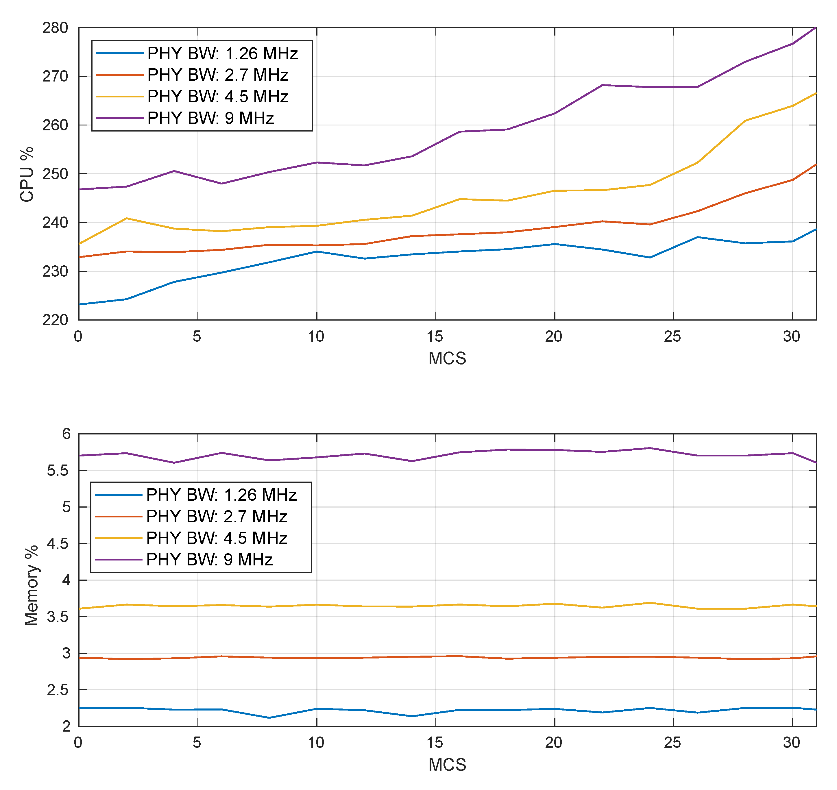
Figure 12 depicts the memory and CPU utilization of SCATTER PHY, using 1.27 , 2.7 , 4.5 , and 9 MHz bandwidths for several MCS values. The results presented in the figure were obtained by averaging memory and CPU usage values. The memory and CPU usage values were sampled every 200 ms for the experiment’s duration. In this experiment, we had SCATTER PHY operating in full-duplex mode, where one PHY transmitted to the other and vice versa. Each one of the PHYs transmitted 20 subframes in a row with a 1 ms gap between transmissions.
As can be noticed, as the selected PHY Tx BW increased, both CPU and memory utilization also increased; however, there was no memory nor CPU starvation for any of the used MCS and PHY Tx BW values. As can be also seen, for a given PHY Tx BW, as the MCS value increased, the CPU usage also increased. This was because the turbo encoding, turbo decoding, and synchronization processing tasks demanded much more CPU power for data processing as the MCS value increased, i.e., as data rates increased. For an MCS equal to 31 and a PHY Tx BW of 9 MHz, the CPU utilization of SCATTER PHY was approximately equal to 280%. That means that less than three CPU cores were being used, consequently leaving the other cores underused for long intervals.
In the case of memory usage, it can be noticed that for a given PHY Tx BW, the memory utilization was almost constant for all MCS values, and therefore, it was practically independent of the selected MCS value. This result was expected once all the RAM memory used by SCATTER PHY was pre-allocated during its initialization. Therefore, based on the results presented in Figure 12, it can be concluded that SCATTER PHY did not exhaust memory or CPU resources as the configured MCS or PHY Tx BW values increased.
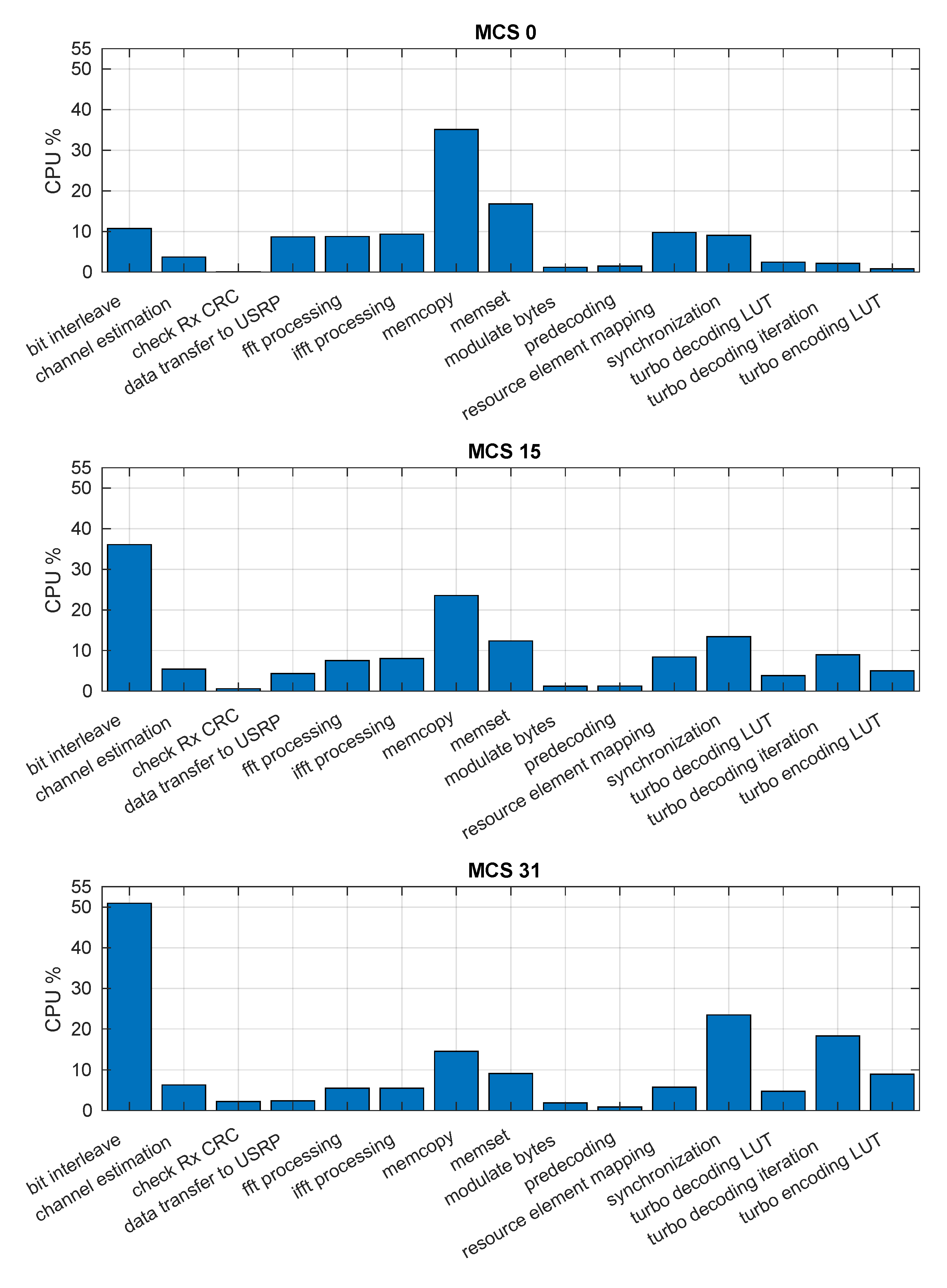
Figure 13 presents the results of the CPU consumption for the main SCATTER PHY’s functions for three different MCS values and a PHY Tx BW of 4.5 MHz. We used valgrind with its callgrind tool for the assessment of the CPU consumption [27]. This experiment used the same setup used for the profiling of memory and CPU. The figure highlights the Rx and Tx functions with highest CPU processing load. By analyzing the figure, we see that the bit interleaving processing used more CPU as the MCS value increased. As can be seen, the CPU time-usage was approximately 11% when the MCS value was set to zero; however, it increased to approximately 51% when the MCS value was set to 31. The synchronization processing task required a considerable amount of CPU time for all considered MCS values. The CPU time consumption for the synchronization ranged from 9% to more than 23%. The CPU time for the synchronization was independent of the selected MCS due to the fact that this processing did not involve data coding/decoding. It can be also noticed that the turbo decoding iteration task consumed more CPU time as the MCS increased, going from 2% (MCS 0) to more than 18% (MCS 31). Additionally, we see that memory copy and setting functions consumed less CPU time as the MCS value increased. This was due to the fact that other functions started consuming more CPU when the MCS increased.

5. Conclusions

The paper described the design, features, and benefits of SCATTER PHY, which is an open-source physical layer that uses a filtered form of OFDM as its waveform.
The main features included using Google’s Protobuf to define the message format for interaction with higher layers of the system and the ability to transmit/receive two different types of packets, which can include a synchronization signal, control data, and user data. The PHY layer communication operated with various modulation and coding schemes, several different channel bandwidths, and automatically improved the carrier frequency offset correction by utilizing the OFDM CP in addition to the synchronization subframe detected in the signal. SCATTER PHY minimized OOBE by utilizing custom-built FPGA based FIR filters on the transmitter side, configured for each channel bandwidth at run-time. Additionally, two independent physical interfaces were available, which effectively enabled the usage of full-duplex and theoretically double the possible throughput achieved with one interface.
The described benefits were verified experimentally. The throughput achieved with actual physical transmissions was compared to a theoretical maximum, defined by using the entire available time for communication with an effective duty cycle of 100%. The verification showed that using full-duplex had no impact on the achieved throughput in each interface. Spectrometer measurement results showcased the capabilities of the FPGA based FIR filter, resulting in negligible OOBE, which in turn increased channel utilization and facilitated communication in neighboring channels by other radios. Using CP based CFO estimation and correction was demonstrated to outperform the sync-signal based correction in all cases, at the expense of higher processing time. Finally, the packet reception rate for all types of transmitted signals was presented, showing that SCATTER PHY could successfully decode user data at SNR values as low as 0 dB.

Author Contributions

Conceptualization, methodology, software, validation, investigation, formal analysis, data curation, and writing, original draft preparation: F.A.P.d.F., D.S., and P.M.; writing, review and editing: R.M., and I.J.; resources, supervision, project administration, and funding acquisition: X.J., and I.M.

Funding

This work was funded by the European Union’s Horizon 2020 research and innovation program under Grant Agreement No. 732174—Orchestration and Reconfiguration Control Architecture (ORCA) project.

Conflicts of Interest

The authors declare no conflict of interest.

Appendix A. Two-Stage Detection Algorithm

The very first processing executed by SCATTER PHY was the detection of incoming synchronization subframes, which might be followed by data-only subframes. This is a task of utmost importance once the correct detection of subframes is crucial in establishing links in scenarios with low SNR or limited by interference. In this Appendix, we describe the proposed detection algorithm employed in SCATTER PHY.
For improved performance, the proposed algorithm was split into two stages. In the first stage, a buffer containing received samples with the length of a subframe was correlated with a local version of the Synch subframe, and then, if the Peak to Side-lobe Ratio (PSR) was greater than or equal to a predefined threshold, Thresh 1 st _ stage , then the detection algorithm proceeded to the second stage. The Power Delay Profile (PDP) between the received signal and the local version of the sync subframe containing only the synchronization signal is defined as:
PDP 1 st _ stage ( l ) = n = 0 N S 1 r [ n ] r l * [ ( n + l ) N S ] 2 , 0 l N S 1 ,
where r ( n ) is the received signal, r l ( n ) is the local version Synch subframe, N S is the length of a subframe, ( . ) N S denotes that this is a cyclic correlation, and ( . ) * is the complex conjugate. Therefore, the detection algorithm proceeds to the second stage if the PSR of the first stage is greater than or equal to the first stage threshold, as defined in (A2). Figure A1 summarizes the processing carried out in the first stage of the synchronization sequence detection algorithm. As is seen in the figure, we used frequency domain cross-correlation as its implementation with FFTs and an IFFT is faster than the time domain version of the correlation [28].
PSR 1 st _ stage = arg max l PDP 1 st _ stage ( l ) arg max i , i l PDP 1 st _ stage ( l ) Thresh 1 st _ stage .
In the second stage, if PSR 1 st _ stage Thresh 1 st _ stage , then the l th lag that maximized the numerator in (A2) possibly points to the middle of the synchronization subframe. Based on the position of the l th lag, it is possible to extract (i.e., convert the Synch OFDM symbol into frequency domain and extract the 72 complex symbols carrying the Synch sequence) the 72 symbol long synchronization sequence and correlate it with its local version as defined next. The PDP between the received Synch sequence and its local version is defined as:
PDP 2 nd _ stage ( m ) = n = 0 N Synch 1 S [ n ] S l * [ ( n + m ) N Synch ] 2 , 0 m N Synch 1 ,
where S ( n ) is the received Synch sequence, S l ( n ) is the local version of the Synch sequence, N Synch is the length of the Synch sequence, ( . ) N Synch denotes that this is a cyclic correlation, and ( . ) * is the complex conjugate. The signal processing carried out at the second stage is based on PDP 2 nd _ stage ( m ) . For the sake of brevity, we use PDP ( m ) to denote PDP 2 nd _ stage ( m ) in what follows.
The second stage of the proposed detection algorithm is based on the CA-CFAR algorithm [20]. It is used to detect the existence of the synchronization sequence within a given received signal buffer. The algorithm is used to calculate a variable detection threshold, which varies according to the noise power, based on the second stage PDP set of samples, PDP 2 nd _ stage ( m ) . The algorithm is divided into three main steps: (i) elimination (i.e., also referred as censoring) of samples that are not regarded as being noise-only (i.e., pure noise samples) observations, (ii) computation of the noise-power threshold level, and finally, (iii) the hypothesis test used to detect the synchronization sequence. These steps make it possible to decide reliably whether the synchronization sequence is present or not in a given received buffer. Figure A2 summarizes the three steps composing the Synch sequence detection algorithm employed in the second stage. Next, we describe each one of the three steps composing the second stage Synch detection algorithm.
The procedure followed in the second-stage of the synchronization sequence detection algorithm essentially involved a hypothesis test that followed the Neyman and Pearson lemma described in [29]. The Neyman and Pearson lemma defines that the hypothesis testing used to detect the presence of synchronization sequence is based on the inequality shown next.
PDP H 1 PDP H 0 > α ,
where the hypothesis H 0 is discarded (i.e., rejected) in favor of the hypothesis H 1 when the PDP set contains the desired signal, i.e., the synchronization sequence. Therefore, the hypothesis H 0 is the one representing the case where only noise is present. The just described hypothesis test is said to be optimum when and only when the Cumulative Distribution Function (CDF) of the ratio in (A4) gives that the hypothesis H 0 is known, so that it is possible to compute a threshold level that fulfil the following equality:
P PDP H 1 PDP H 0 > α | H 0 = P F R ,
for a pre-defined (i.e., given) probability of false-rejection, P F R . Therefore, the calculation of the detection threshold level considers that the Probability Distribution Function (PDF) of both random variables, PDP H 1 and PDP H 0 , is known.
Figure A1. Summary of the first-stage synchronization sequence detection algorithm.
Electronics 08 01343 g0a1
Figure A2. Summary of the second-stage Synch sequence detection algorithm: Step (i) is employed to calculate a reference for the noise-power, Z REF ; Step (ii) is employed to calculate the detection-threshold, α ; and Step (iii) applies a test of hypothesis to the values of the second stage Power Delay Profile (PDP).
Electronics 08 01343 g0a2

Appendix A.1. Step # 1: Censoring and Calculation of the Noise-Power Reference Level

In this first step, PDP samples containing the presence of other than noise observations, i.e., corrupted PDP samples, are removed (i.e., censored) from the PDP reference set. Corrupted samples are caused by the presence of samples containing noise plus another signal (i.e., a signal different from noise). For the discarding/removal of corrupted PDP samples, we employed the algorithm known as Forward Consecutive Mean Excision (FCME) [30]. To begin with, the samples in the PDP set can be defined as:
PDP ( m ) | m = 0 , 1 , , N Synch 1 ,
and then, the PDP samples are sorted in ascending order of values; this way, the sorted PDP set can be defined as:
PDP ( i ) | i = 0 , 1 , , N Synch 1 ,
where:
PDP ( 0 ) PDP ( 1 ) PDP ( 2 ) PDP ( N Synch 1 ) .
The discarding of corrupted PDP samples, at the k th iteration of the algorithm, is carried out through the application of the following inequality:
PDP ( k + 1 ) T k i = 1 k PDP ( i ) ,
where T k corresponds to the discarding/censoring scaling factor at the k th iteration of the censoring algorithm. If the inequality shown in (A9) holds, all the PDP samples that present values greater than PDP ( k + 1 ) are considered to be corrupted. The testing of (A9) is carried out iteratively, where it is necessary to compute the censoring scaling factor, T k , for every new iteration of the algorithm. The discarding scaling factor, T k , rules the properties of the discarding step of the detection algorithm. This parameter is generally chosen in order that the probability of false disposal, P F D , presents a pre-defined value. The probability of making an incorrect decision during the k th iteration of the discarding step is denoted by P F D . The initial value of T k is computed considering that PDP ( k + 1 ) is a PDP sample that does not contain the presence of the synchronization sequence, i.e., a PDP sample containing a noise-only observation. Based on this premise, the probability that the inequality given by (A9) holds corresponds to the probability of false disposal, P F D , defined as:
P F D = P PDP ( k + 1 ) T k i = 1 k PDP ( i ) | H 0 .
Every iteration of the discarding step initializes with the parameter k being equal to the smallest supposed clean set (i.e., noise-only set) of PDP samples. The larger the supposed clean set, the better the discarding algorithm works [30]. However, the larger the supposed clean set is, the higher is the likelihood that corrupted PDP samples (i.e., samples containing other than noisy-only observations) will be part of the initial supposed clean set. The testing of (A9) proceeds until it is true for some value of the parameter k or all PDP samples used as a reference are considered to be noise-only (i.e., signal-free) samples.
Considering the H 0 hypothesis (i.e., observation of samples only containing noise) and that the noise is a stochastic processes following a complex Gaussian distribution, CN ( 0 , σ 2 ) , therefore, each one of the PDP values follows a Gamma distribution, Γ ( 1 , N Synch σ 2 ) with mean given by:
E [ PDP ( . ) ] = N Synch σ 2 .
Therefore, since:
i = 0 k 1 PDP ( i ) k E [ PDP ( . ) ] = N Synch σ 2 ,
the equation defining the probability of false disposal, P F D , can be accurately approximated as:
P F D P PDP ( k + 1 ) T k k N Synch σ 2 .
The approximation given by (A13) becomes more and more accurate as the amount of reference PDP samples, i.e., k, increases. Moreover, given that the PDP sample PDP ( k + 1 ) is a random variable with Gamma distribution, Γ ( k , θ ) , with the shape parameter, k, equal to one, therefore, as demonstrated in [31,32], its CDF can be simplified and expressed in closed-form by:
F ( y , k , θ ) = P ( Y y ) = 1 e y / θ i = 0 k 1 1 i ! y θ i ,
where θ and k are the scale and shape parameters of the Gamma distribution, respectively.
Consequently, the probability of false censoring given by (A13) can be computed as:
P F D = 1 P PDP ( k + 1 ) T k k N Synch σ 2 = e T k k ,
where in (A14), y has been set to T k k N Synch σ 2 . Next, we establish that T C M E = k T k , where T C M E is an input parameter to the FCME algorithm and is computed by solving (A15). Therefore, the probability of false censoring, P F D , can be thought of as the desired rejection rate to obtain a clean sample set.
The censoring/discarding threshold level is defined as T k i = 1 k PDP ( i ) . This way, PDP samples that present values greater than or equal to the threshold level are censored (i.e., removed from the set). Next, the new set of samples consists of samples that are considered to be noise-only observations. The outcome of the discarding step consists of (i) the noise-power reference level, Z REF , and (ii) the number of noise-only samples, k. The noise-power reference level is computed as the summation of all PDP samples that present values that are less than the discarding threshold level. The noise-power reference level, Z REF , is given by:
Z REF = i = 1 k PDP ( i ) .

Appendix A.2. Step # 2: Calculation of the Detection Threshold Level

Following the computation of the noisy-only set of PDP samples, in Step # 1 of the algorithm, the next step of the algorithm involves computing the synchronization detection threshold level, α . The synchronization detection threshold level, α , is computed following the decision method known in the literature as the Cell Averaging (CA) method [30].
The synchronization detection threshold level, α , is computed assuming that there is no synchronization sequence present within the set of PDP reference samples for a given probability of false alarm, P F A . The probability of false alarm, P F A , is given by:
P F A = P PDP ( i ) Z REF α | H 0 .
Next, we consider that the noise-power reference, Z REF , and the PDP samples both follow scaled central Chi-squared distributions, given by N Synch σ 2 2 χ 2 ( 2 k ) and N Synch σ 2 2 χ 2 ( 2 ) with 2 k and 2 degrees of freedom, respectively. Moreover, it is known from the theory of random variables that the ratio of two central Chi-squared random variables results in a random variable that exhibits a Fisher distribution [30,33], whose CDF is given by:
FCDF ( α ) = 1 P PDP ( i ) / 2 Z REF / 2 k k α ,
consequently, the synchronization detection threshold level, α , is computed as:
α = FCDF 1 ( 1 P F A , 2 , 2 k ) / k .
where FCDF represents the CDF of the Fisher distribution. It is important to notice that the scaling factor given by N Synch σ 2 2 is the same for Z REF and PDP ( . ) , and consequently, it vanishes when the ratio of the two central Chi-squared random variables is taken.

Appendix A.3. Step # 3: Detection of the Synchronization Sequence

Finally, after the calculation of the noise-power reference, Z REF , and the synchronization sequence detection threshold level, α , the decision about whether the synchronization sequence is present or not is evaluated through the following hypothesis testing:
PDP ( i ) α Z REF , i = 0 , 1 , , N Synch 1 .
If the hypothesis testing is true, then the synchronization sequence plus noise hypothesis, H 1 , is selected. Otherwise, if the hypothesis testing is false, then the noise-only hypothesis, H 0 , is selected, and consequently, the received signal buffer is proclaimed as not having the presence of the synchronization sequence.

Appendix A.4. Results of the Synchronization Sequence Detection Algorithm

In this section, we present some results when the synchronization sequence detection algorithm is employed. Figure A3 presents a comparison between the expected P F A and the actual P F A value. The expected P F A was varied from 10 5 to 10 4 . The number of Monte Carlo trials was set to 10 6 iterations, and an AWGN channel was assumed. As can be seen, the actual P F A value stayed very close to the expected one.
Figure A4 depicts P F A versus the probability of correct detection, P C D . The P F A was varied from 10 5 to 10 4 ; the SNR was set to 0 dB; and the number of Monte Carlo trials was equal to 10 5 iterations. The figure shows that the presence of a synchronization sequence was always detected independent of the P F A value set.
Figure A3. Comparison between the expected P F A and the actual value for an SNR of 0 dB.
Electronics 08 01343 g0a3
Figure A4. Comparison between P F A and the actual P C D value for an SNR of 0 dB.
Electronics 08 01343 g0a4
Next, we present some results comparing the detection performance of the proposed two-stage detection algorithm against the single-stage one. The number of Monte Carlo trials here was set to 10 5 iterations, and the AWGN channel was used. For both results shown in Figure A5, the probability of false alarm P F A was set to 10 4 , and the probability of false disposal P F D was set to 10 3 . Figure 5a shows the correct and misdetection probabilities for the SNR varying from 12 dB up to 0 dB. As can be noticed, the proposed two-stage detection scheme presented a probability of correct detection of one for SNR values greater than 4 dB, i.e., the presence of the synchronization sequence was always detected, while the single scheme only achieved a probability of one for SNR values greater than 2 dB. Figure 5b shows the correct miss and false detection probabilities when the noise power varied from 30 dBW up to 0 dBW. As can be seen, both schemes presented the correct miss probability equal to one and the false detection probability equal to zero for all noise power values considered in this experiment. It is important to be mentioned that the combined working of the two detection stages decreased the probability of false detection (also known as false alarm) of the two-stage algorithm when compared to the probability of false detection of the second stage alone (see Figure A3).
Figure A5. Comparison between the single- and two-stage synchronization sequence detection schemes: (a) correct and misdetection probabilities; (b) correct miss and false detection probabilities.
Electronics 08 01343 g0a5

Appendix B. CFO Estimation

Appendix B.1. Integer Estimation

After Synch signal detection and subframe alignment, the integer (i.e., coarse) CFO estimation was carried out by correlating the received OFDM symbol carrying the Synch signal with several local versions of it with different integer frequency offset applied to each of them. The PDP between the received and a given offset local version of the Synch OFDM symbol is defined as:
PDP ( l , k IFO ) = n = 0 N FFT 1 y [ n ] x l * [ ( n + l ) N FFT ] e j 2 π k IFO n N FFT 2 , 0 l N FFT 1 36 k IFO 36 ,
where x l ( n ) is the offset local version of the Synch symbol, y ( n ) is the received Synch OFDM symbol signal, N FFT is the FFT length, ( . ) N FFT denotes that this is a cyclic correlation, k IFO is the integer frequency offset, and ( . ) * is the complex conjugate. Therefore, the integer frequency offset can be estimated by solving the following maximization problem:
ϵ ^ k IFO = arg max k IFO arg max l PDP ( l , k IFO ) .
Figure A6 shows the performance of the integer CFO estimation algorithm described above for an AWGN channel over several SNR values and a PHY BW of 4.5 MHz.
Figure A6. Performance of the integer CFO estimation algorithm.
Electronics 08 01343 g0a6

Appendix B.2. Fractional Estimation

As shown by the results in Figure 8, the CP based fractional CFO estimation outperformed the Synch based fractional CFO one and therefore was the method adopted by SCATTER PHY. Next, we describe the CP based fractional CFO estimation.
ψ ( k ) = n = 0 N CP 1 r d * ( n + k ( N FFT + N CP ) ) r d ( n + k ( N FFT + N CP ) + N FFT ) 2 π ,
ϵ ^ FFO = 1 N symb k = 0 N symb 1 arg ψ ( k ) ,
where r d ( n ) is the detected, integer CFO corrected, and aligned subframe, N symb is the number of OFDM symbols used to average the CFO estimation, and N CP is the length of the OFDM cyclic prefix. As can be seen, the employed CP based fractional CFO estimation was obtained by averaging the estimated fractional CFO over the selected number of OFDM symbols.

References

  1. DARPA SC2. DARPA Spectrum Collaboration Challenge. Available online: Https://spectrumcollaborationchallenge.com/ (accessed on 17 September 2019).
  2. Stojadinovic, D.; de Figueiredo, F.A.P.; Maddala, P.; Seskar, I.; Trappe, W. SC2 CIL: Evaluating the Spectrum Voxel Announcement Benefits. In Proceedings of the IEEE International Symposium on Dynamic Spectrum Access Networks (DySPAN2019), Newark, NJ, USA, 11–14 November 2019. [Google Scholar]
  3. Giannoulis, S.; Donato, C.; Mennes, R.; de Figueiredo, F.A.P. Dynamic and Collaborative Spectrum Sharing: The SCATTER Approach. In Proceedings of the IEEE International Symposium on Dynamic Spectrum Access Networks (DySPAN2019), Newark, NJ, USA, 11–14 November 2019. [Google Scholar]
  4. Mennes, R.; Claeys, M.; de Figueiredo, F.A.P.; Jabandzic, I.; Moerman, I.; Latre, S. Deep Learning-Based Spectrum Prediction Collision Avoidance for Hybrid Wireless Environments. IEEE Access 2019, 7, 45818–45830. [Google Scholar] [CrossRef]
  5. Hintjens, P. ZeroMQ Messaging for Many Applications; O’Reilly Media: Sebastopol, CA, USA, March 2013. [Google Scholar]
  6. De Figueiredo, F.A.P.; Mennes, R.; Jiao, X.; Liu, W.; Moerman, I. A spectrum sharing framework for intelligent next-generation wireless networks. IEEE Access 2018, 6, 60704–60735. [Google Scholar] [CrossRef]
  7. De Figueiredo, F.A.P.; Stojadinovic, D.; Maddala, P.; Mennes, R.; Jabandžic, I.; Jiao, X.; Moerman, I. SCATTER PHY: An Open Source Physical Layer for the DARPA Spectrum Collaboration Challenge. Available online: Https://github.com/zz4fap/scatter-phy (accessed on 17 September 2019).
  8. Yu, Y.; Wang, T.; Liew, S.C. Deep-Reinforcement Learning Multiple Access for Heterogeneous Wireless Networks. In Proceedings of the IEEE International Conference on Communications (ICC), Kansas City, MO, USA, 20–24 May 2018. [Google Scholar]
  9. Mennes, R.; Camelo, M.; Claeys, M.; Latre, S. A Neural-Network based MF-TDMA MAC Scheduler for Collaborative Wireless Networks. In Proceedings of the IEEE Wireless Communications and Networking Conference (WCNC), Barcelona, Spain, 15–18 April 2018. [Google Scholar]
  10. Camelo, M.; Shahid, A.; Fontaine, J.; de Figueiredo, F.A.P.; de Poorter, E.; Moerman, I.; Latre, S. A Semi-Supervised Learning Approach Towards Automatic Wireless Technology Recognition. In Proceedings of the IEEE International Symposium on Dynamic Spectrum Access Networks (DySPAN), Newark, NJ, USA, 11–14 November 2019. [Google Scholar]
  11. Ta, D.T.; Nguyen-Thanh, N.; Nguyen, V.T.; Nguyen, D. Collaborative Paradigm for Next Generation Wireless Networks. EURASIP J. Wirel. Commun. Netw. Available online: https://hal.archives-ouvertes.fr/hal-01713174 (accessed on 20 February 2018).
  12. Jang, S.J.; Han, C.H.; Lee, K.E.; Yoo, S.J. Reinforcement learning based dynamic band and channel selection in cognitive radio ad-hoc networks. EURASIP J. Wirel. Commun. Netw. 2019, 131. [Google Scholar] [CrossRef]
  13. Ettus Research LLC. USRP Hardware Driver. Available online: http://files.ettus.com/manual/ (accessed on 27 August 2019).
  14. Ettus Research LLC. USRP X Series. Available online: https://www.ettus.com/product/category/USRP-X-Series (accessed on 27 August 2019).
  15. National Instruments. Overview of the NI USRP RIO Software-Defined Radio. White Paper. 2015. Available online: http://www.ni.com/white-paper/52119/en/ (accessed on 27 August 2019).
  16. Ettus Research LLC. Products. Available online: https://www.ettus.com/product (accessed on 27 August 2019).
  17. Google. protobuf—Protocol Buffers—Google’s Data Interchange Format. 2011. Available online: http://code.google.com/p/protobuf/ (accessed on 27 August 2019).
  18. Gomez-Miguelez, I.; Garcia-Saavedra, A.; Sutton, P.D.; Serrano, P.; Cano, C.; Leith, D.J. srsLTE: An Open-Source Platform for LTE Evolution and Experimentation. In Proceedings of the ACM WiNTECH Workshop, New York City, NY, USA, 3–7 October 2016. [Google Scholar]
  19. Kanchi, S.; Sandilya, S.; Bhosale, D.; Pitkar, A.; Gondhalekar, M. Overview of LTE-A technology. In Proceedings of the IEEE Global High Tech Congress on Electronics (GHTCE), Shenzhen, China, 17–19 November 2014. [Google Scholar]
  20. De Figueiredo, F.A.P.; Cardoso, F.A.C.M.; Bianco, F.J.A.; Vilela, R.M.; Lenzi, K.G. Multi-stage Based Cross-Correlation Peak Detection for LTE Random Access Preambles. Rev. Telecomun. 2013, 15, 21–27. [Google Scholar]
  21. Chu, D.C. Polyphase codes with good periodic correlation properties. IEEE Trans. Inf. Theory 1972, 18, 531–532. [Google Scholar] [CrossRef]
  22. Sarwate, D.V.; Pursley, M.B. Crosscorrelation properties of pseudorandom and related sequences. Proc. IEEE 1980, 68, 593–619. [Google Scholar] [CrossRef]
  23. Wang, F.; Zhu, Y. An efficient CFO estimation algorithm for the downlink of 3GPP-LTE. In Proceedings of the International Conference on Wireless Communications and Signal Processing (WCSP), Nanjing, China, 9–11 November 2011. [Google Scholar]
  24. Bodinier, Q.; Bader, F.; Palicot, J. On Spectral Coexistence of CP-OFDM and FB-MC Waveforms in 5G Networks. IEEE Access 2017, 5, 13883–13900. [Google Scholar] [CrossRef]
  25. Lin, H.; Siohan, P. Major 5G Waveform Candidates: Overview and Comparison. In Signal Processing for 5G; Wiley: Hoboken, NJ, USA, 2016. [Google Scholar]
  26. Ettus Research LLC. CBX 1200-6000 MHz Rx/Tx (120 MHz, X Series Only). Available online: Https://www.ettus.com/product/details/CBX120 (accessed on 5 September 2019).
  27. Weidendorfer, J.; Kowarschik, M.; Trinitis, C. A Tool Suite for Simulation Based Analysis of Memory Access Behavior. In Proceedings of the 4th International Conference on Computational Science (ICCS), Krakow, Poland, 6–9 June 2004. [Google Scholar]
  28. Sesia, S.; Toufik, I.; Baker, M. LTE—The UMTS Long Term Evolution: From Theory to Practice; John Wiley & Sons: Hoboken, NJ, USA, 2011. [Google Scholar]
  29. Neyman, J.; Pearson, E.S. On the problem of the most efficient tests of statistical hypotheses. Philos. Trans. R. Soc. Lond. Ser. A 1933, 231, 289–337. [Google Scholar] [CrossRef]
  30. Lehtomaki, J.J.; Juntti, M.; Saarnisaari, H. CFAR Strategies for Channelized Radiometer. IEEE Signal Process. Lett. 2005, 12, 13–16. [Google Scholar] [CrossRef]
  31. Proakis, J.G. Digital Communications, 5th ed.; McGraw-Hill: New York, NY, USA, 2001. [Google Scholar]
  32. Papoulis, A.; Pillai, S.U. Probability, Random Variables, and Stochastic Processes, 4th ed.; McGraw-Hill Europe: New York, NY, USA, 2002. [Google Scholar]
  33. DeGroot, M.H. Probability and Statistics, 2nd ed.; Addison-Wesley: Boston, MA, USA, 1986. [Google Scholar]
Figure 1. High level threading architecture of SCATTER PHY.
Electronics 08 01343 g001
Figure 2. Block-diagram showing the modules making up the transmitter and receiver sides of the SCATTER PHY.
Electronics 08 01343 g002
Figure 3. SCATTER PHY frame structure. COT, Channel Occupancy Time.
Electronics 08 01343 g003
Figure 4. Closer coexistence to other radios due to reduced Out-Of-Band Emissions (OOBE).
Electronics 08 01343 g004
Figure 5. Comparison of the McF-TDMA scheme with and without filtering. (a) FPGA based filters disabled. (b) The 128 order FPGA based filters enabled.
Electronics 08 01343 g005
Figure 6. SCATTER PHY throughput for several Tx bandwidths and Modulation Code Scheme (MCS) values.
Electronics 08 01343 g006
Figure 7. Comparison between unfiltered and filtered based COT transmissions. (a) Spectrogram without filtering. (b) Spectrum without filtering. (c) Spectrogram with filtering enabled. (d) Spectrum with filtering enabled.
Electronics 08 01343 g007
Figure 8. Comparison of CFO estimation error (MAPE) in the AWGN channel.
Electronics 08 01343 g008
Figure 9. Comparison of the Packet Reception Rate (PRR) for the different signals carried by a SCATTER PHY subframe.
Electronics 08 01343 g009
Figure 10. Simple Rx combined with SCATTER PHY for several PHY BW values.
Electronics 08 01343 g010
Figure 11. Comparison of the variation of the maximum number of turbo decoding iterations for a PHY Tx BW of 1.27 MHz and three different MCS values.
Electronics 08 01343 g011
Figure 12. CPU and memory utilization of SCATTER PHY.
Electronics 08 01343 g012
Figure 13. CPU profiling of SCATTER PHY for a PHY Tx BW of 4.5 MHz.
Electronics 08 01343 g013
Table 1. OFDM modulation parameters.
PHY BW (MHz)1.262.74.59
Subframe duration (ms)1
subcarrier spacing (kHz)15
Sample rate (Msps)1.923.845.7611.52
FFT size128256384768
Useful subcarriers84180300600
OFDM symbols per subframe14
CP duration ( μ s)4.69 (12 symbols)/5.21 (2 symbols)
Table 2. Modulation code schemes and their respective code rates. MCS, Modulation Code Scheme.
Code Rate
MCSModulation1.26 MHz2.7 MHz4.5 MHz9 MHz
0QPSK0.08570.09000.09400.0940
1QPSK0.11430.12000.12200.1220
2QPSK0.13570.14670.14800.1480
3QPSK0.17140.19330.19200.1920
4QPSK0.21070.24000.24000.2440
5QPSK0.25710.29330.29600.2920
6QPSK0.30710.34000.34400.3440
7QPSK0.35710.40000.41600.4130
8QPSK0.40710.46670.46400.4690
9QPSK0.47140.52000.53600.5330
1016QAM0.23570.26000.26800.2665
1116QAM0.25710.29330.29200.2905
1216QAM0.30000.32670.32800.3305
1316QAM0.33570.36670.38000.3825
1416QAM0.38570.42670.42900.4298
1516QAM0.42860.46670.47700.4718
1616QAM0.44290.50000.50900.5078
1764QAM0.29520.33330.33930.3385
1864QAM0.32380.36000.35530.3625
1964QAM0.35240.39110.40330.4087
2064QAM0.39050.44110.43530.4407
2164QAM0.42860.46780.47270.4727
2264QAM0.45710.51220.50470.5100
2364QAM0.49520.54780.55700.5642
2464QAM0.53330.58330.59700.6042
2564QAM0.57140.61890.62100.6308
2664QAM0.59050.66330.66900.6770
2764QAM0.61900.69000.70100.7010
2864QAM0.65710.80560.80670.8178
2964QAM0.69520.83220.82800.8552
3064QAM0.73330.86170.84930.8925
3164QAM0.77140.88830.87070.9240
Table 3. List of real-time configurable parameters and statistics provided by SCATTER PHY.
MessageParameterTypeUnitRange
Tx controlPHY IDuint32-0–1
MCSuint8-0–28
Tx gainuint32dBdepends on HW 1
Tx channeluint32- 0
Tx PHY BWuint8MHz0–3 2
Transmission timestampuint64s 0
User Data lengthuint32- > 0
User datauchar[]-uchar range
Rx controlPHY IDuint32-0–1
Rx channeluint32- 0
Rx gainuint32dBdepends on HW 1
Rx PHY BWuint8MHz0–3 2
Max. # of turbo decoder iterationsuint32-uint32 range
Enable Rx combiningBoolean-True/false
Rx statisticsPHY IDuint32-0–1
CQIuint8-0–15
RSSIfloatdBWfloat range
NoisefloatdBWfloat range
Decoded MCSuint8-0–28
Subframe error counteruint32- 0
Decoding timeuint32ms 0
Data lengthuint32- 0
# of turbo decoder iterationsuint32-uint32 range
Received datauchar[]-uchar range
Tx statisticsPHY IDuint32-0–1
Coding timeuint32ms 0
Number of transmitted subframesuint32- 0
1 This parameter depends on the installed USRP daughter board model [16]. 2 The numbers correspond to the following bandwidths: 1.26 , 2.7 , 4.5 , and 9 MHz, respectively.

