Correlated Blocking in mmWave Cellular Networks: Macrodiversity, Outage, and Interference

Abstract

In this paper, we provide a comprehensive analysis of macrodiversity for millimeter wave (mmWave) cellular networks. The key issue with mmWave networks is that signals are prone to blocking by objects in the environment, which causes paths to go from line-of-sight (LOS) to non-LOS (NLOS). We identify macrodiversity as an important strategy for mitigating blocking, as with macrodiversity the user will attempt to connect with two or more base stations. Diversity is achieved because if the closest base station is blocked, then the next base station might still be unblocked. However, since it is possible for a single blockage to simultaneously block the paths to two base stations, the issue of correlated blocking must be taken into account by the analysis. Our analysis characterizes the macrodiverity gain in the presence of correlated random blocking and interference. To do so, we develop a framework to determine distributions for the LOS probability, Signal to Noise Ratio (SNR), and Signal to Interference and Noise Ratio (SINR) by taking into account correlated blocking. We validate our framework by comparing our analysis, which models blockages using a random point process, with an analysis that uses real-world data to account for blockage. We consider a cellular uplink with both diversity combining and selection combining schemes. We also study the impact of blockage size and blockage density along with the effect of co-channel interference arising from other cells. We show that the assumption of independent blocking can lead to an incorrect evaluation of macrodiversity gain, as the correlation tends to decrease macrodiversity gain.

1. Introduction

Millimeter-wave (mmWave) has emerged in recent years as a viable candidate for infrastructure-based (i.e., cellular) systems [1,2,3,4,5]. Communicating at mmWave frequencies is attractive due to the potential to support high data rates at low latency [1,2,6]. At mmWave frequencies, signals are prone to blocking by objects intersecting the paths and severely reducing the signal strength, and thus the Signal to Noise Ratio (SNR) [7,8,9,10]. For instance, blocking by walls provides isolation between indoor and outdoor environments, making it difficult for an outdoor base station to provide coverage indoors [11]. To mitigate the issue of blocking in mmWave cellular networks, macrodiversity has emerged as a promising solution, where the user attempts to connect to multiple base stations [12]. With macrodiversity, the probability of having at least one line-of-sight (LOS) path to a base station increases, which can improve the system performance [13,14,15].

An effective methodology to study wireless systems in general, and mmWave systems in particular, is to embrace the tools of stochastic geometry to analyze the SNR and interference in the network [3,15,16,17,18,19,20]. With stochastic geometry, the locations of base stations and blockages are assumed to be drawn from an appropriate point process, such as a Poisson point process (PPP). When blocking is modeled as a random process, the probability that a link is LOS is an exponentially decaying function of link distance. While many papers assume that blocking is independent [11,17], in reality the blocking of multiple paths may be correlated [18]. The correlation effects are especially important for macrodiverity networks when base stations are close to each other, or more generally when base stations have a similar angle to the transmitter. In this case, when one base station is blocked, there is a significant probability that another base station is also blocked [13,14,15].

Prior work has considered the SINR distribution of mmWave personal networks [16,17,21]. Such work assumes that the blockages are drawn from a point process (or, more specifically, that the centers of the blockages are drawn from a point process and each blockage is characterized by either a constant or random width). Meanwhile, the transmitters are either in fixed locations or their locations are also drawn from a point process. A universal assumption in this prior art is that the blocking is independent; i.e., each transmitter is blocked independently from the other transmitters. As blocking has a major influence on the distribution of signals, it must be carefully taken into account. Independent blocking is a crude approximation that fails to accurately capture the true environment, especially when the base stations, or, alternatively, the user equipments (UEs), are closely spaced in the angular domain or when there are few sources of blocking. We note that blocking can be correlated even when the sources of blockage are placed independently according to a point process.

The issue of blockage correlation was considered in [22,23,24,25], but it was in the context of a localization application where the goal was to ensure that a minimum number of positioning transmitters were visible by the receiver. As such, this prior work was only concerned with the number of unblocked transmissions rather than the distribution of the received aggregate signal (i.e., source or interference power). In [18], correlated blocking between interferers was considered for wireless personal area network. Recently, correlation between base stations was considered in [13,14] for infrastructure-based networks with macrodiversity, but in these references the only performance metric considered is the nth order LOS probability; i.e., the probability that at least one of the n closest base stations is LOS. However, a full characterization of performance requires other important performance metrics, including the distributions of the SNR and, when there is interference, the Signal to Interference and Noise Ratio (SINR). Alternatively, the performance can be characterized by the coverage probability, which is the complimentary cumulative distribution function of the SNR or SINR, or the rate distribution, which can be found by using information theory to link the SNR or SINR to the achievable rate.

In this paper, we propose a novel approach for fully characterizing the performance of macrodiversity in the presence of correlated blocking. While, like [13,14], we are able to characterize the spatially averaged LOS probability (i.e., the LOS probability averaged over many network realizations), our analysis shows the distribution of the LOS probability, which is the fraction of network realizations that can guarantee a threshold LOS probability rather than its mere spatial average. Moreover, we are able to similarly capture the distributions of the SNR and SINR. Furthermore we validate our framework by comparing the analysis to a real data building model.

We assume that the centers of the blockages are placed according to a PPP. We first analyze the distributions of LOS probability for first- and second-order macrodiversity. We then consider the distribution of SNR and SINR for the cellular uplink with both selection combining and diversity combining. The signal model is such that blocked signals are completely attenuated, while LOS, i.e., non-blocked, signals are subject to an exponential path loss and additive white Gaussian noise (AWGN). Though it complicates the exposition and notation, the methodology can be extended to more elaborate models, such as one wherein all signals are subject to fading and non-LOS (NLOS) signals are partially attenuated (see, e.g., [17]).

The remainder of the paper is organized as follows. We begin by providing the system model in Section 2, wherein there are base stations and blockages, each drawn from a PPP. In Section 3 we provide an analysis of the LOS probability under correlated blocking and derive the blockage correlation coefficient using arguments based on the geometry and the properties of the blockage point process; i.e., by using stochastic geometry. Section 4 provides a framework of the distribution of SNR, where the results depend on the blockage correlation coefficient. In Section 5, we validate our framework by comparing the analysis to a real data model. Then in Section 6, interference is considered and the SINR distribution is formalized. Finally, Section 7 concludes the paper, suggesting extensions and generalizations of the work.

2. System Model

2.1. Network Topology

Consider a mmWave cellular network consisting of base stations, blockages, and a source transmitter, which is a UE. The UE attempts to connect to the N closest base stations, and therefore operates in a $N$th order macrodiversity mode. The locations of the base stations are modeled as an infinite homogeneous PPP with density ${\lambda }_{bs}$. We assume the centers of the blockages also form a homogeneous PPP with density ${\lambda }_{bl}$, independent from the base station process. Let $Y_0$ indicate the source transmitter and its location. Due to the stationarity of the PPPs, and without loss of generality, we can assume the coordinates are chosen such that the source transmitter is located at the origin; i.e., $Y_0=0$. In Section 6, we will consider additional transmitters located in neighboring cells, which act as interferers.

Let $X_i$ for i $\in {\mathbb{Z}}^{+}$ denote the base stations and their locations. Let $R_i=\left|X_i\right|$ be the distance from $Y_0$ to $X_i$. Base stations are ordered according to their distances to $Y_0$ such that $R_1\le R_2\le \dots$. The signal of the source transmitter is received at the closest N base stations, and hence, N is the number of $X_i$ connected to $Y_0$. For a PPP, a derivation of the distribution of $R_1,\dots ,R_N$ is given in Appendix B, which implies a methodology for generating these distances within a simulation.

Figure 1 shows an example of second-order macrodiversity ($N=2$) cellular network where the user attempts to connect to its closest two base stations. The solid line indicates the link from the user to the base station is LOS, while the dashed line indicates the link is NLOS. The figure shows examples of two different blockage scenarios. In Figure 1a the closest base station ($X_1$) is LOS while $X_2$ is NLOS to the user, in which case the blockage only blocks a single link. In Figure 1b a single blockage blocks both links to $X_1$ and $X_2$. The fact that sometimes a single blockage can block both links is an illustration of the effect of correlated blocking.

2.2. Blockage Model

As in [18], each blockage is a segment of length W. To capture the worst-case scenario, as shown in Figure 2a, it is assumed that the line representing the blockage is perpendicular to the line that connects it to the transmitter. Although W can itself be random as in [13], we assume here that all blockages have the same value of W. In Figure 2a, the red stars indicate the blocked base stations, which are located in the blue shaded region. If a blockage cuts the path from $Y_0$ to $X_i$, then the signal from $Y_0$ is NLOS, while otherwise it is LOS. Here, we assume that NLOS signals are completely blocked while LOS signals experience exponential path-loss with a path-loss exponent $\alpha$; i.e., the power received by $X_i$ is proportional to $R_i^{-\alpha }$.

Each base station has a blockage region associated with it, illustrated by the blue shaded rectangles shown in Figure 2b. We use $a_i$ to denote the blockage region associated with $X_i$ and its area; i.e., $a_i$ is both a region and an area. If the center of a blockage falls within $a_i$, then $X_i$ will be blocked since at least some part of the blockage will intersect the path between $X_i$ and $Y_0$. Because $a_i$ is a rectangle of length $R_i$ and width W, it is clear that $a_i=W{R}_i$. Unless $X_1$ and $X_2$ are exactly on opposite sides of the region, there will be an overlapping region v common to both $a_1$ and $a_2$. Because of the overlap, it is possible for a single blockage to simultaneously block both $X_1$ and $X_2$ if the blockage falls within region v, which corresponds to correlated blocking.

3. LOS Probability Analysis Under Correlated Blocking

In this section, we analyze the LOS probability, which is denoted $p_{LOS}$, and the impact of blockage correlation. Our focus is on second-order macrodiversity, where the signal of the source transmitter $Y_0$ is received at the two closest base stations $X_1$ and $X_2$. The LOS probability is the probability that at least one $X_i$ is LOS to the transmitter. Because the base stations are randomly located, the value of $p_{LOS}$ will vary from one network realization to the next, or equivalently by a change of coordinates, from one source transmitter location to the next. Hence, $p_{LOS}$ is itself a random variable and must be described by a distribution. To determine $p_{LOS}$ and its distribution, we first need to define the variable $B_i$ which indicates that the path between $Y_0$ and $X_i$ is blocked. Let $p_{B_1,B_2}(b_1,b_2)$ be the joint probability mass function (pmf) of $\{B_1,B_2\}$. Let $p_i$ denote the probability that $B_i=1$, which indicates the link from $Y_0$ to $X_i$ is NLOS. Furthermore, let $q_i=1-p_i$, which is the probability that the link is LOS, and $\rho$ denote the correlation coefficient between $B_1$ and $B_2$. As shown in Appendix A, the joint pmf of $\{B_1,B_2\}$ as a function of $\rho$ found to be

$$\begin{array}{ccc}\hfill p_{B_1,B_2}(b_1,b_2)& =& \left\{\begin{array}{cc}{q}_1{q}_2+\rho h\hfill & for b_1=0,b_2=0\hfill \\ q_1{p}_2-\rho h\hfill & for b_1=0,b_2=1\hfill \\ p_1{q}_2-\rho h\hfill & for b_1=1,b_2=0\hfill \\ p_1{p}_2+\rho h\hfill & for b_1=1,b_2=1\hfill \end{array}\right.\hfill \end{array}$$

(1)

where $h=\sqrt{p_1{p}_2{q}_1{q}_2}$.

For a two-dimensional homogeneous PPP with density $\lambda$, the number of points within an area a is Poisson with mean $\lambda a$ [26]. From the probability mass function of a Poisson variable, the probability of k points within the area is given by [27]

$$\begin{array}{c}\hfill p_K\left(k\right)=\frac{{\left(\lambda a\right)}^k}{k!}{e}^{-\lambda a}\end{array}$$

(2)

The event that the path to $X_i$ is not blocked (LOS) by an object falling in area $a_i$ can be obtained by the void probability of PPP, which is the probability that there are no blockages located in $a_i$, or equivalently, the probability that $k=0$. Thus, $q_i$, which is equal to the void probability, is given by substituting $k=0$ into (2) with $\lambda ={\lambda }_{bl}$ and $a=a_i$, which results in

$$\begin{array}{c}\hfill q_i=exp(-{\lambda }_{bl}{a}_i)\end{array}$$

(3)

For first-order macrodiversity ($N=1$), the LOS probability is given by $q_1$. Conversely, $X_i$ will be NLOS when at least one blockage lands in $a_i$ and this occurs with probability $p_i=1-q_i$ given by

$$\begin{array}{c}\hfill p_i=1-exp(-{\lambda }_{bl}{a}_i)\end{array}$$

(4)

For second-order macrodiversity (N = 2), there will be a LOS signal as long as both paths are not blocked. This corresponds to the case that $B_1$ and $B_2$ are both not equal to unity. When blocking is not correlated, the corresponding LOS probability is $1-p_1{p}_2$. Correlated blocking may be taken into account by using (1) and noting that the LOS probability is the probability that $B_1$ and $B_2$ are not both equal to one, which is given by

$$\begin{array}{c}\hfill p_{LOS}=1-p_{B_1,B_2}(1,1)=1-p_1{p}_2-\rho h\end{array}$$

(5)

The blockage correlation coefficient $\rho$ can be found from (1),

$$\begin{array}{ccc}\hfill \rho & =& \frac{p_{B_1,B_2}(0,0)-q_1{q}_2}{h}\hfill \end{array}$$

(6)

where $p_{B_1,B_2}(0,0)$ is the probability that both $X_1$ and $X_2$ are LOS. Looking at Figure 2b, this can occur when there are no blockages inside $a_1$ and $a_2$. Taking into account the overlap v, this probability is the void probability for area $(a_1+a_2-v)$, which is given by

$$\begin{array}{c}\hfill p_{B_1,B_2}(0,0)=e^{-{\lambda }_{bl}(a_1+a_2-v)}\end{array}$$

(7)

Details on how to compute the overlapping area v are provided in [18]. Substituting (7) into (6) into (5) and using the definitions of $p_i$ and $q_i$ yields

$$\begin{array}{c}\hfill p_{LOS}=e^{-{\lambda }_{bl}{a}_1}+e^{-{\lambda }_{bl}{a}_2}-e^{-{\lambda }_{bl}(a_1+a_2-v)}\end{array}$$

(8)

Let $\theta$ be the angular separation between $X_1$ and $X_2$. The relationship between the angular separation $\theta$ and the correlation coefficient $\rho$ is illustrated in Figure 3 using an example. In the example, the distances from the source transmitter to the two base stations are fixed at $R_1=1.2$ and $R_2=1.5$ and the base station density is ${\lambda }_{bs}=0.3$. In Figure 3a, we fixed the blockage density at ${\lambda }_{bl}=0.6$, and the blockage width W is varied. In Figure 3b, $W=0.5$ and the value of ${\lambda }_{bl}$ is varied. Both figures show that $\rho$ decreases with increasing $\theta$. This is because the area v gets smaller as $\theta$ increases. As $\theta$ approaches 180 degrees, v approaches zero, and the correlation is minimized. The figures show that correlation is more dramatic when W is large, since a single large blockage is likely to simultaneously block both base stations, and when ${\lambda }_{bl}$ is small, which corresponds to the case that there are fewer blockages.

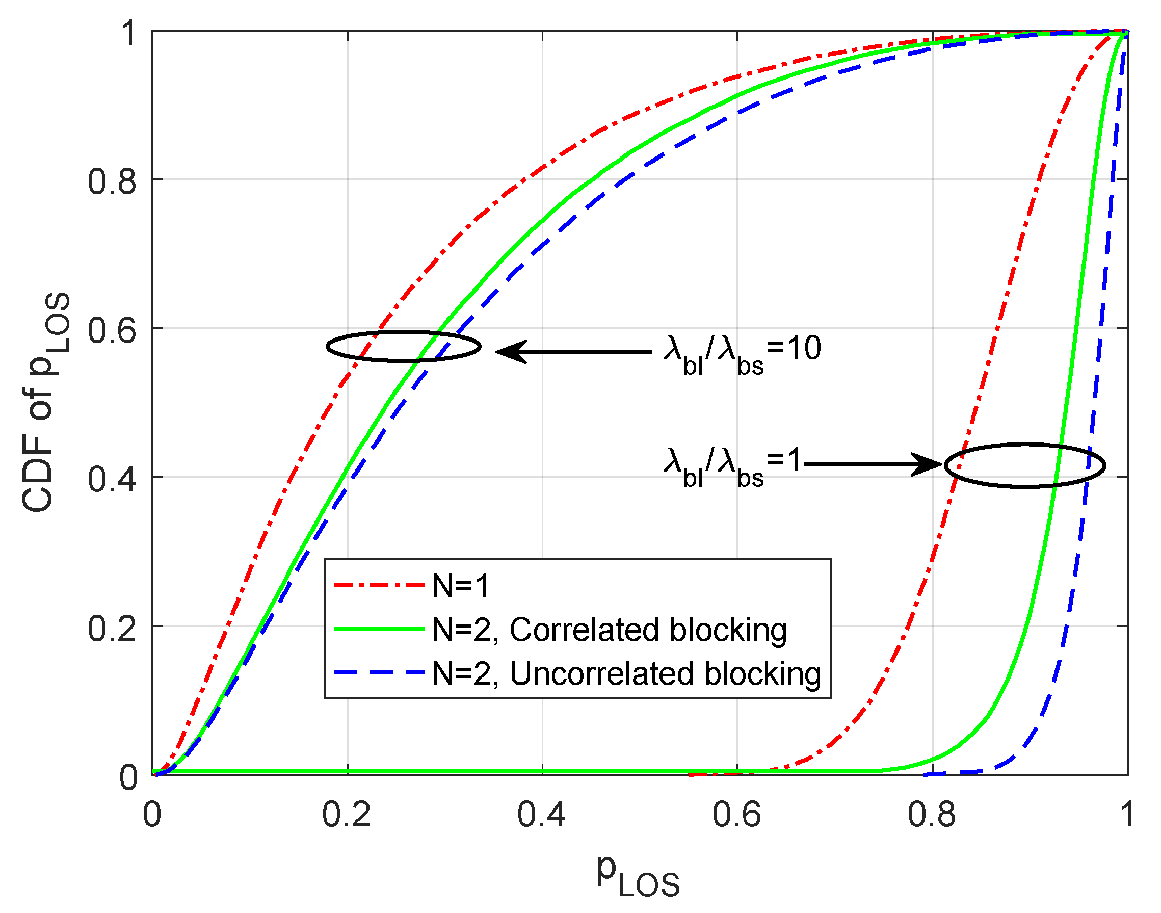
Figure 4 shows the empirical cumulative distribution function (CDF) of $p_{LOS}$ over 1000 network realizations for first- and second-order macrodiversity, both with and without considering blockage correlation. The distributions are computed by fixing the value of $W=0.8$ and using two different values of the average number of blockages per base station (${\lambda }_{bl}/{\lambda }_{bs}$). The CDF of $p_{LOS}$ quantifies the likelihood that the $p_{LOS}$ is below some value. The figure shows the probability that $p_{LOS}$ is below some value increases significantly when the number of blockages per base station is high. The effect of correlated blocking is more pronounced when there are fewer blockages per base station. The macrodiversity gain is the improvement in performance for $N=2$ as compared to $N=1$, in the figure the macrodiversity gain is higher when the number of blockages per base station is lower even though the amount of reduction in gain due to correlation is higher when ${\lambda }_{bl}/{\lambda }_{bs}$ is lower.

Figure 5 shows the variation of $p_{LOS}$ when averaged over 1000 network realizations. In this figure, 1000 $p_{LOS}$ values is found for different 1000 network realization, then the averaged $p_{LOS}$ is calculated for different values of blockage density ${\lambda }_{bl}$. The derivation of the distances for each network realization can be found in Appendix B. The plot shows average $p_{LOS}$ as a function of ${\lambda }_{bl}$ while keeping base station density ${\lambda }_{bs}$ fixed at 0.3. The spatially averaged $p_{LOS}$ is computed for two different values of blockage width W. Compared to the case of no diversity (when $N=1$), the second-order macrodiversity can significantly increase $p_{LOS}$. However, $p_{LOS}$ decreases when blockage size or blockage density is higher. Moreover, correlated blocking reduces the $p_{LOS}$ compared to independent blocking, and larger blockages increase the correlation, since a single large blockage is likely to simultaneously block both base stations. Comparing the two pairs of correlated/uncorrelated blocking curves, the correlation is more dramatic when ${\lambda }_{bl}$ is low, since at low ${\lambda }_{bl}$ both base stations are typically blocked by the same blockage (located in area v).

4. SNR Distribution

In this section, we consider the distribution of the SNR. Macrodiversity can be achieved by using either diversity combining, where the signals from the multiple base stations are maximum ratio combined, or selection combining, where only the signal with the strongest SNR is used. For $n$th-order macrodiversity, the SNR with diversity combining is [28]

$$\begin{array}{c}\hfill \mathsf{SNR}={\mathsf{SNR}}_0\underset{Z}{\underbrace{{\sum }_{i=1}^n(1-B_i){\mathsf{\Omega }}_i}}\end{array}$$

(9)

where ${\mathsf{\Omega }}_i=R_i^{-\alpha }$ is the power gain between the source transmitter $Y_0$ to the $i$th base station and ${\mathsf{SNR}}_0$ is the SNR of an unblocked reference link of unit distance. $B_i$ is used to indicate that the path between $Y_0$ and $X_i$ is blocked, and thus when $B_i=1$, ${\mathsf{\Omega }}_i$ does not factor into the SNR.

The CDF of SNR, $F_{\mathsf{SNR}}\left(\beta \right)$, quantifies the likelihood that the combined SNR at the closest n base stations is below some threshold $\beta$. If $\beta$ is interpreted as the minimum acceptable SNR required to achieve reliable communications, then $F_{\mathsf{SNR}}\left(\beta \right)$ is the outage probability of the system $P_o\left(\beta \right)=F_{\mathsf{SNR}}\left(\beta \right)$. The coverage probability is the complimentary CDF, $P_c\left(\beta \right)=1-F_{\mathsf{SNR}}\left(\beta \right)$ and is the likelihood that the SNR is sufficiently high to provide coverage. The rate distribution can be found by linking the threshold $\beta$ to the transmission rate, for instance by using the appropriate expression for channel capacity.

The CDF of SNR evaluated at threshold $\beta$ is as follows:

$$\begin{array}{c}\hfill F_{\mathsf{SNR}}\left(\beta \right)=P\left[\mathsf{SNR}\le \beta \right]=P\left[Z\le \frac{\beta }{{\mathsf{SNR}}_0}\right]=F_Z\left(\frac{\beta }{{\mathsf{SNR}}_0}\right).\end{array}$$

(10)

The discrete variable Z represents the sum of the unblocked signals. To find the CDF of Z we need to find the probability of each value of Z, which is found as follows for second-order macrodiversity. The probability that $Z=0$ can be found by noting that $Z=0$ when both $X_1$ and $X_2$ are blocked. From (1), this is

$$\begin{array}{c}\hfill p_Z\left(0\right)=p_{B_1,B_2}(1,1)=p_1{p}_2+\rho h.\end{array}$$

(11)

The probability that $Z={\mathsf{\Omega }}_i,i\in \{1,2\}$ can be found by noting that $Z={\mathsf{\Omega }}_i$ when only $X_i$ is LOS. From (1), this is

$$\begin{array}{ccc}\hfill p_Z\left({\mathsf{\Omega }}_1\right)& =& p_{B_1,B_2}(0,1)=q_1{p}_2-\rho h.\hfill \end{array}$$

(12)

$$\begin{array}{ccc}\hfill p_Z\left({\mathsf{\Omega }}_2\right)& =& p_{B_1,B_2}(1,0)=p_1{q}_2-\rho h.\hfill \end{array}$$

(13)

Finally, by noting that $Z={\mathsf{\Omega }}_1+{\mathsf{\Omega }}_2$ when both $X_1$ and $X_2$ are LOS leads to

$$\begin{array}{ccc}\hfill p_Z\left({\mathsf{\Omega }}_1+{\mathsf{\Omega }}_2\right)& =& p_{B_1,B_2}(0,0)=q_1{q}_2+\rho h.\hfill \end{array}$$

(14)

From (11) to (14), the CDF of Z is found to be:

$$\begin{array}{c}\hfill F_Z\left(z\right)=\left\{\begin{array}{cc}0\hfill & \mathrm{for}z<0\hfill \\ p_1{p}_2+\rho h\hfill & \mathrm{for}0\le z<{\mathsf{\Omega }}_2\hfill \\ p_1\hfill & \mathrm{for}{\mathsf{\Omega }}_2\le z<{\mathsf{\Omega }}_1\hfill \\ p_1+q_1{p}_2-\rho h\hfill & \mathrm{for}{\mathsf{\Omega }}_1\le z<{\mathsf{\Omega }}_1+{\mathsf{\Omega }}_2\hfill \\ 1\hfill & \mathrm{for}z\ge {\mathsf{\Omega }}_1+{\mathsf{\Omega }}_2.\hfill \end{array}\right.\end{array}$$

(15)

Next, in the case of selection combining, the SNR is [28]

$$\begin{array}{c}\hfill \mathsf{SNR}={\mathsf{SNR}}_0\underset{Z}{\underbrace{\max \left[(1-B_1){\mathsf{\Omega }}_1,(1-B_2){\mathsf{\Omega }}_2,\cdots ,(1-B_n){\mathsf{\Omega }}_n\right]}}\end{array}$$

(16)

and its CDF, from (11) to (13), is found for second-order macrodiversity to be:

$$\begin{array}{c}\hfill F_Z\left(z\right)=\left\{\begin{array}{cc}0\hfill & \mathrm{for}z<0\hfill \\ p_1{p}_2+\rho h\hfill & \mathrm{for}0\le z<{\mathsf{\Omega }}_2\hfill \\ p_1\hfill & \mathrm{for}{\mathsf{\Omega }}_2\le z<{\mathsf{\Omega }}_1\hfill \\ 1\hfill & \mathrm{for}z\ge {\mathsf{\Omega }}_1.\hfill \end{array}\right.\end{array}$$

(17)

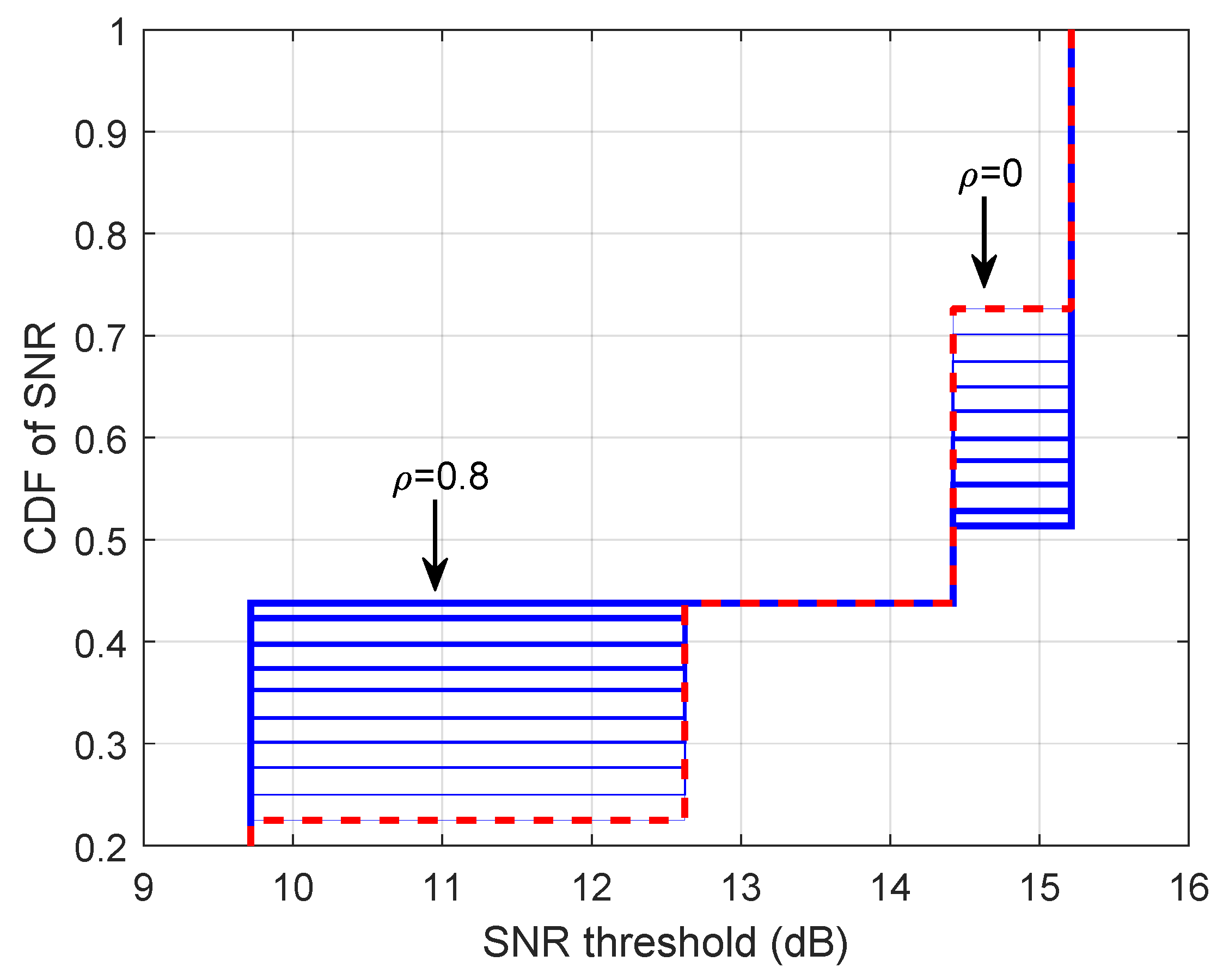
Figure 6 is an example showing the effect that the value of the correlation coefficient $\rho$ has upon the CDF of SNR. The curves were computed by placing the base stations at distances $R_1=2$ and $R_2=5$, and fixing the values of $\alpha =2$ and ${\mathsf{SNR}}_0=15$ dB. The values of $q_i$ and $p_i$ were computed using (3) and (4) respectively, by assuming $W=0.6$, ${\lambda }_{bl}=0.3$. The CDF is found assuming values of $\rho$ between $\rho =0$ to $\rho =0.8$ in increments of 0.1; the value of $\rho$ can be adjusted by varying the angle $\theta$ between the two base stations. The dashed red line represents the case that $\rho =0$, corresponding to uncorrelated blocking. The solid blue lines correspond to positive values of $\rho$ in increments of 0.1, where the thinnest line corresponds to $\rho =0.1$ and the thickest line corresponds to $\rho =0.8$.

Figure 6 shows a first step up at $9.7$ dB, and the increment of the step is equal to the probability that both base stations are NLOS. The magnitude of the step gets larger as the blocking is more correlated, because correlation increases the chance that both base stations are NLOS (i.e., $p_{B_1,B_2}(1,1)$). The next step up occurs at $12.7$ dB, which is the SNR when just one of the two closest base stations is blocked, which in this case is the closest base station $X_1$. The next step at $14.5$ dB represents the case when only $X_2$ is blocked, The magnitude of the two jumps is equal to the probability that only the corresponding one base station is LOS, and this magnitude decreases with positive correlation, because if one base station is LOS the other one is NLOS. Finally, there is a step at 15.2 dB, which corresponds to the case that both base stations are LOS. Notice that when $\rho =0.8$, the two middle steps merge. This is because for such a high value of, it is impossible for just one base station to be blocked, and most likely that both base stations are blocked, so the curve goes directly from SNR = 9.7 dB to SNR = 15.2 dB.

Figure 7 shows the CDF of SNR over 1000 network realizations for diversity combining and two different values of W when ${\lambda }_{bs}=0.4$ and ${\lambda }_{bl}=0.6$. In addition, ${\mathsf{SNR}}_0$ and the path loss $\alpha$ are fixed at 15 dB and 3 respectively for the remaining figures in this paper. It can be observed that the CDF increases when blockage size is larger. Compared to the case when $N=1$, the use of second-order macrodiversity decreases the SNR distribution. When compared to uncorrelated blocking, correlation decreases the gain of macrodiversity for certain regions of the plot, particularly at low values of SNR threshold, corresponding to the case when both base stations are blocked. Similar to $p_{LOS}$, the correlation increases with blockage size. However, the macrodiversity gain is slightly higher when blockage width W is smaller.

Figure 8 shows the effect of combining scheme and ${\lambda }_{bl}$ on SNR outage probability at threshold $\beta =10$ dB. As shown in the figure, the outage probability increases when ${\lambda }_{bl}$ increases in all of the given scenarios. When ${\lambda }_{bl}=0$, first- and second-order selection combining perform identically. This is because $X_1$ is never blocked. However, as ${\lambda }_{bl}$ increases, the gain of both selection combining and diversity combining increase. At high ${\lambda }_{bl}$ the combining scheme is less important, in which case the paths to $X_1$ and $X_2$ are always blocked regardless of the chosen combining scheme. The reduction in gain due to correlation is slightly higher when using selection combining. From Equation (17) this is because the step when both base stations are blocked is wider compared to diversity combining case.

5. Real Data Validation

To validate our framework, we consider a region of West Virginia University campus as shown in Figure 9 with base stations locations drawn from a PPP and a randomly placed user. The exterior walls of the buildings highlighted in red color are considered to be the blockages. The equivalent parameters for the statistical analysis introduced by this paper are obtained by calculating the number of buildings, the area of each building, and the total area of the region. The average blockage width (W) is found from the areas of the individual buildings ($A_i$), such that the width of each blockage $W_i=2\sqrt{A_i/\pi }$, while the blockage density is found as the the number of buildings divided by the total region area.

Figure 10 shows the empirical CDF of SNR over 1000 network realizations computed using our statistical analysis and computed using the actual data. The total region area is found to be $335,720$ m${}^2$, the number of buildings is 49, the average building width is $W=33$ m, ${\lambda }_{bl}$ is the ratio of number of buildings to the total area, and ${\lambda }_{bs}=3{\lambda }_{bl}$. We limited the environment to be outdoor by allowing the base stations and user to only be located outside buildings. It can be observed that the analysis approximates the performance in the real scenario very well. Compared to the curves representing the analysis when $N=2$, it is clear that the real data model when $N=2$ is closer to the case when considering correlated blocking compared to the case assuming independent blocking. This is because one building can simultaneously block more than one base station. In the actual region, the blockages have different sizes and orientations, this is in contrast with our model, which assumes a constant blockage size and orientation. Due to these differences, there is a small different between the statistical model and the real data based model as shown in the figure.

6. SINR Outage Analysis

Thus far, we have not assumed any interfering transmitters in the system. In practice, the received signal is also affected by the sum interference. The goal of this section is to formulate the CDF of SINR for second-order macrodiversity. SINR for first-order macrodeiversity along with blockage correlation between interferers has been considered in [15]. In this section, we assume each neighboring cell has a single interfering mobile, which is located uniformly within a disk of radius r around the base station. Assuming a perfect packing of cells, $r={\left({\lambda }_{bs}\pi \right)}^{-1/2}$, which is the average cell radius. We explicitly consider the interference from the M closest neighboring cells. The interference from more distant cells is considered to be part of the thermal noise. Let $Y_j$ for $j=1,2,..,M$ indicate the interfering transmitters and their locations. Recall that $j=0$ indicates the source transmitter $Y_0$. The distance from the $j$th transmitter to the $i$th base station is denoted by $R_{i,j}$.

To calculate SINR and its distribution, we first define a matrix $\mathbf{B}$ which indicates the blocking state of the paths from $Y_j$ for $j=0,2,..,M$ to $X_i$ for $i=1,2$. $\mathbf{B}$ is a Bernoulli Matrix of size 2 by $(M+1)$ elements. Each column in $\mathbf{B}$ contain elements $B_{1,j}$ and $B_{2,j}$ which indicate the blocking states of the paths from $Y_j$ to $X_1$ and $X_2$ respectively; i.e, the first column in $\mathbf{B}$ contains the pair of Bernoulli random variables $B_{1,0}$ and $B_{2,0}$ that indicates the blocking state of the paths from $Y_0$ to $X_i$ for $i=1,2$. There are $(M+1)$ pairs of Bernoulli random variables, and each pair is correlated with correlation coefficient ${\rho }_j$. Because the $2(M+1)$ elements of $\mathbf{B}$ are binary, there are $2^{2(M+1)}$ possible combinations of $\mathbf{B}$. However, it is possible for different realizations of $\mathbf{B}$ to correspond to the same value of SINR. For example, when $X_1$ and $X_2$ are both blocked from $Y_0$, the SINR will be the same value regardless of the blocking states of the interfering transmitters. Define ${\mathbf{B}}^{\left(n\right)}$ for $n=1,2,\dots ,2^{2(M+1)}$ to be the $n$th such combination of $\mathbf{B}$. Similar to Section 3, let $p_{B_{1,j},B_{2,j}}(b_{1,j}^{\left(n\right)},b_{2,j}^{\left(n\right)})$ be the joint probability of $B_{1,j}$ and $B_{2,j}$ which are the elements of the $j$th column of ${\mathbf{B}}^{\left(n\right)}$. The probability of ${\mathbf{B}}^{\left(n\right)}$ is given by

$$\begin{array}{c}\hfill P\left(B^{\left(n\right)}\right)=\prod _{j=0}^M{p}_{B_{1,j},B_{2,j}}(b_{1,j}^{\left(n\right)},b_{2,j}^{\left(n\right)})\end{array}$$

(18)

The SINR of a given realization ${\mathbf{B}}^{\left(n\right)}$ at base station $X_i$ is given by

$$\begin{array}{c}\hfill {\mathsf{SINR}}_i^{\left(n\right)}=\frac{(1-B_{i,0}^{\left(n\right)}){\mathsf{\Omega }}_{i,0}}{{\displaystyle {\mathsf{SNR}}_0^{-1}+\sum _{j=1}^M(1-B_{i,j}^{\left(n\right)}){\mathsf{\Omega }}_{i,j}}}\end{array}$$

(19)

where ${\mathsf{\Omega }}_{i,j}=R_{i,j}^{-\alpha }$ is the path gain from the $j$th transmitter at the $i$th base station. The SINR of the combined signal considering selective combining is expressed as

$$\begin{array}{c}\hfill {\mathsf{SINR}}^{\left(n\right)}=\mathsf{max}\left({\mathsf{SINR}}_1^{\left(n\right)},{\mathsf{SINR}}_2^{\left(n\right)}\right)\end{array}$$

(20)

When considering diversity combining (20) changes to

$$\begin{array}{c}\hfill {\mathsf{SINR}}^{\left(n\right)}\le {\mathsf{SINR}}_1^{\left(n\right)}+{\mathsf{SINR}}_2^{\left(n\right)}\end{array}$$

(21)

As described in [29], correlated interference tends to make the combined $\mathsf{SINR}$ less than the sum of the individual SINRs. The bound in (21) is satisfied with equality when the interference is independent at the two base stations.

To generalize the formula for any realization, there is a particular ${\mathsf{SINR}}^{\left(n\right)}$ associated with each ${\mathbf{B}}^{\left(n\right)}$. However, as referenced above, multiple realizations of ${\mathbf{B}}^{\left(n\right)}$ may result in the same SINR. Let ${\mathsf{SINR}}^{\left(k\right)}$ be the $k$th realization of $\mathsf{SINR}$. Its probability is

$$\begin{array}{c}\hfill P\left({\mathsf{SINR}}^{\left(k\right)}\right)=\sum _{\begin{array}{c}n:\mathsf{SINR}={\mathsf{SINR}}^{\left(k\right)}\end{array}}P\left(B^{\left(n\right)}\right)\end{array}$$

(22)

Figure 11 shows the distributions of SINR for $M=5$ and $M=0$ (which is SNR) at fixed values of ${\lambda }_{bs}=0.3$, ${\lambda }_{bl}=0.6$, and $W=0.6$. The distributions are computed for first- and second-order macrodiversity. It can be observed that macrodiversity gain is reduced when interference is considered. This is because of the increase in sum interference due to macrodiversity, which implies that $p_{LOS}$ alone as in [13] may not be sufficient to predict the performance of the system especially when there are many interfering transmitters. Study of higher order macrodiversity to identify the minimum order of macrodiversity to achieve a desired level of performance in the presence of interference is left for future work.

Figure 12 shows the variation of SINR outage probability with respect to the number of interfering transmitters M. The curves are computed for low and high values of ${\lambda }_{bl}$, while keeping ${\lambda }_{bs}$ and W fixed at $0.8$ and $0.6$ respectively. It can be seen that the outage probability increases when M increases. Due to the fact that interference tends to also be blocked, unlike SNR and $p_{LOS}$, increasing the ${\lambda }_{bl}$ decreases the outage probability. Similar to Figure 11, the macrodiversity gain decreases significantly when M increases. It can be seen that $N=2$ curves reaches the case when $N=1$ for $M=6$. Compared to uncorrelated blocking, the curves considering correlated blocking matches the uncorrelated cases for high value of M, since the interfering transmitters are placed farther than source transmitter and their overlapping area is less dominant.

7. Conclusions

We have proposed a framework to analyze the second-order macrodiversity gain for an mmWave cellular system in the presence of correlated blocking. Correlation is an important consideration for macrodiversity because a single blockage can block multiple base stations, especially if the blockage is sufficiently large and the base stations sufficiently close. The assumption of independent blocking leads to an incorrect evaluation of macrodiversity gain of the system. By using the methodology in this paper, the correlation between two base stations is found and factored into the analysis. The paper considered the distributions of LOS probability, SNR, and, when there is interference, the SINR. The framework was confirmed by comparing the analysis to a real data model. We show that correlated blocking decreases the macrodiversity gain. We also study the impact of blockage size and blockage density. We show that blockage can be both a blessing and a curse. On the one hand, the signal from the source transmitter could be blocked, and on the other hand, interfering signals tend to also be blocked, which leads to a completely different effect on macrodiversity gains.

The analysis can be extended in a variety of ways. In Section 6, we have already shown that any number of interfering transmitters can be taken in to account. While this paper has focused on the extreme case that LOS signals are AWGN while NLOS signals are completely blocked, it is possible to adapt the analysis to more sophisticated channels, such as those where both LOS and NLOS signals are subject to fading and path loss, but the fading and path loss parameters are different depending on the blocking state. See, for instance, [17] for more detail. We may also consider the use of directional antennas, which will control the effect of interference [30].

Finally, while this paper focused on second-order macrodiversity, the study can be extended to the more general case of an arbitrary macrodiversity order. Such a study could identify the minimum macrodiversity order required to achieve desired performance in the presence of interference. We anticipate that when more than two base stations are connected, the effects of correlation on macrodiversity gain will increase and the effect of interference will decrease. This is because the likelihood that two base stations are close together increases with the number of base stations and the ratio of the number of connected base stations to the number of interfering transmitters will increase.

References

1. Rappaport, T.S.; Sun, S.; Mayzus, R.; Zhao, H.; Azar, Y.; Wang, K.; Wong, G.N.; Schulz, J.K.; Samimi, M.; Gutierrez, F. Millimeter wave mobile communications for 5G cellular: It will work. IEEE Access 2013, 1, 335–349. [Google Scholar] [CrossRef]
2. Akdeniz, M.R.; Liu, Y.; Samimi, M.K.; Sun, S.; Rangan, S.; Rappaport, T.S.; Erkip, E. Millimeter Wave Channel Modeling and Cellular Capacity Evaluation. IEEE J. Sel. Areas Commun. 2014, 32, 1164–1179. [Google Scholar] [CrossRef]
3. Andrews, J.G.; Bai, T.; Kulkarni, M.N.; Alkhateeb, A.; Gupta, A.K.; Heath, R.W., Jr. Modeling and Analyzing Millimeter Wave Cellular Systems. IEEE Trans. Commun. 2017, 65, 403–430. [Google Scholar] [CrossRef]
4. Park, J.; Andrews, J.G.; Heath, R.W. Inter-Operator Base Station Coordination in Spectrum-Shared Millimeter Wave Cellular Networks. IEEE Trans. Cogn. Commun. Netw. 2018, 4, 513–528. [Google Scholar] [CrossRef]
5. Singh, S.; Kulkarni, M.N.; Ghosh, A.; Andrews, J.G. Tractable Model for Rate in Self-Backhauled Millimeter Wave Cellular Networks. IEEE J. Sel. Areas Commun. 2015, 33, 2196–2211. [Google Scholar] [CrossRef]
6. Jurdi, R.; Gupta, A.K.; Andrews, J.G.; Heath, R.W. Modeling Infrastructure Sharing in mmWave Networks With Shared Spectrum Licenses. IEEE Trans. Cogn. Commun. Netw. 2018, 4, 328–343. [Google Scholar] [CrossRef] [Green Version]
7. Rappaport, T.; Heath, R.W., Jr.; Daniels, R.C.; Murdock, J.N. Millimeter Wave Wireless Communications; Pearson Education: Upper Saddle River, NJ, USA, 2014. [Google Scholar]
8. Fisher, R. 60 GHz WPAN Standardization within IEEE 802.15.3c. In Proceedings of the International Symposium on Signals, Systems and Electronics, Montreal, QC, Canada, 30 July–2 August 2007; pp. 103–105. [Google Scholar]
9. Singh, S.; Ziliotto, F.; Madhow, U.; Belding, E.; Rodwell, M. Blockage and directivity in 60 GHz wireless personal area networks: From cross-layer model to multihop MAC design. IEEE J. Sel. Areas Commun. 2009, 27, 1400–1413. [Google Scholar] [CrossRef]
10. Niu, Y.; Li, Y.; Jin, D.; Su, L.; Wu, D. Blockage Robust and Efficient Scheduling for Directional mmWave WPANs. IEEE Trans. Veh. Technol. 2015, 64, 728–742. [Google Scholar] [CrossRef]
11. Bai, T.; Vaze, R.; Heath, R.W., Jr. Analysis of Blockage Effects on Urban Cellular Networks. IEEE Trans. Wirel. Commun. 2014, 13, 5070–5083. [Google Scholar] [CrossRef] [Green Version]
12. Choi, J. On the Macro Diversity With Multiple BSs to Mitigate Blockage in Millimeter-Wave Communications. IEEE Commun. Lett. 2014, 18, 1653–1656. [Google Scholar] [CrossRef]
13. Gupta, A.K.; Andrews, J.G.; Heath, R.W. Macrodiversity in Cellular Networks With Random Blockages. IEEE Trans. Wirel. Commun. 2018, 17, 996–1010. [Google Scholar] [CrossRef]
14. Gupta, A.K.; Andrews, J.G.; Heath, R.W. Impact of Correlation between Link Blockages on Macro-Diversity Gains in mmWave Networks. In Proceedings of the IEEE International Conference on Communications Workshops, Kansas City, MO, USA, 20–24 May 2018. [Google Scholar]
15. Hriba, E.; Valenti, M.C. The Potential Gains of Macrodiversity in mmWave Cellular Networks with Correlated Blocking. In Proceedings of the IEEE Military Communications Conference (MILCOM), Norfolk, VA, USA, 12–14 November 2019. [Google Scholar]
16. Venugopal, K.; Valenti, M.C.; Heath, R.W., Jr. Device-to-Device Millimeter Wave Communications: Interference, Coverage, Rate, and Finite Topologies. IEEE Trans. Wirel. Commun. 2016, 15, 6175–6188. [Google Scholar] [CrossRef]
17. Hriba, E.; Valenti, M.C.; Venugopal, K.; Heath, R.W. Accurately Accounting for Random Blockage in Device-to-Device mmWave Networks. In Proceedings of the IEEE Global Telecommunications Conference (GLOBECOM), Singapore, 4–8 December 2017. [Google Scholar]
18. Hriba, E.; Valenti, M.C. The Impact of Correlated Blocking on Millimeter-Wave Personal Networks. In Proceedings of the IEEE Military Communications Conference (MILCOM), Los Angeles, CA, USA, 29–31 October 2018. [Google Scholar]
19. Thornburg, A.; Heath, R.W. Ergodic Rate of Millimeter Wave Ad Hoc Networks. IEEE Trans. Wirel. Commun. 2018, 17, 914–926. [Google Scholar] [CrossRef]
20. Baccelli, F.; Błaszczyszyn, B.; Muhlethaler, P. An Aloha protocol for multihop mobile wireless networks. IEEE Trans. Inf. Theory 2006, 52, 421–436. [Google Scholar] [CrossRef] [Green Version]
21. Venugopal, K.; Valenti, M.C.; Heath, R.W., Jr. Interference in finite-sized highly dense millimeter wave networks. In Proceedings of the Information Theory and Applications Workshop (ITA), San Diego, CA, USA, 1–6 February 2015; pp. 175–180. [Google Scholar]
22. Aditya, S.; Dhillon, H.S.; Molisch, A.F.; Behairy, H. Asymptotic Blind-Spot Analysis of Localization Networks Under Correlated Blocking Using a Poisson Line Process. IEEE Wirel. Commun. Lett. 2017, 6, 654–657. [Google Scholar] [CrossRef] [Green Version]
23. Aditya, S.; Dhillon, H.S.; Molisch, A.F.; Behairy, H.M. A Tractable Analysis of the Blind Spot Probability in Localization Networks Under Correlated Blocking. IEEE Trans. Wirel. Commun. 2018, 17, 8150–8164. [Google Scholar] [CrossRef] [Green Version]
24. Talarico, S.; Valenti, M.C.; Di Renzo, M. Outage Correlation in Finite and Clustered Wireless Networks. In Proceedings of the IEEE International Symposium on Personal, Indoor and Mobile Radio Communications (PIMRC), Bologna, Italy, 9–12 September 2018; pp. 1–7. [Google Scholar]
25. Samuylov, A.; Gapeyenko, M.; Moltchanov, D.; Gerasimenko, M.; Singh, S.; Himayat, N.; Andreev, S.; Koucheryavy, Y. Characterizing Spatial Correlation of Blockage Statistics in Urban mmWave Systems. In Proceedings of the IEEE Globecom Workshops, Washington, DC, USA, 4–8 December 2016; pp. 1–7. [Google Scholar]
26. Snyder, D.L.; Miller, M.I. Random Point Processes in Time and Space, 2nd ed.; Springer Texts in Electrical Engineering: New York, NY, USA, 1991. [Google Scholar]
27. Leon-Garcia, A. Probability and Random Processes for Electrical Engineering, 3rd ed.; Pearson: Boston, MA, USA, 2008. [Google Scholar]
28. Goldsmith, A. Wireless Communications; Cambridge University Press: New York, NY, USA, 2005. [Google Scholar]
29. Tanbourgi, R.; Dhillon, H.S.; Andrews, J.G.; Jondral, F.K. Effect of Spatial Interference Correlation on the Performance of Maximum Ratio Combining. IEEE Trans. Wirel. Commun. 2014, 13, 3307–3316. [Google Scholar] [CrossRef] [Green Version]
30. Torrieri, D.; Talarico, S.; Valenti, M.C. Analysis of a Frequency-Hopping Millimeter-Wave Cellular Uplink. IEEE Trans. Wirel. Commun. 2016, 15, 7089–7098. [Google Scholar] [CrossRef]
Figure 1. Example network topology with two different blockage scenarios. The source transmitter is the mobile device shown in the central cell. Its signal is transmitted to its closest two base stations. The solid line indicates the link is line-of-sight (LOS), while the dashed line indicates the link is non-LOS (NLOS).
Electronics 08 01187 g001
Figure 2. Illustration of the blockage model. (a) Network example consisting of base stations indicated by the stars and blockages indicated by blue lines surrounding the transmitter, which is indicated by the black circle. The blockages are modeled as a line of length W facing the transmitter; (b) Equivalent blockage regions. a 1 and a 2 are the blockage areas, and v is the overlapping area.
Electronics 08 01187 g002
Figure 3. The correlation coefficient ( ρ ) versus the angular separation ( θ ) between X 1 and X 2 .
Electronics 08 01187 g003
Figure 4. The empirical cumulative distribution function (CDF) of p L O S over 1000 network realizations when N = 1 , 2 , with and without considering blockage correlation at fixed blockage width W = 0 . 8 .
Electronics 08 01187 g004
Figure 5. The variation of the spatially averaged p L O S over 1000 network realizations with respect to blockage density λ b l when N = 1 , 2 , with and without considering blockage correlation at fixed base station density λ b s = 0 . 3 .
Electronics 08 01187 g005
Figure 6. The CDF of the Signal to Noise Ratio (SNR) F SINR ( β ) using diversity combining for fixed location of X 1 and X 2 for different values of ρ . The dashed red line shows the CDF when ρ = 0 , and the solid blue lines correspond to positive values of ρ in increments of 0.1.
Electronics 08 01187 g006
Figure 7. The distribution of SNR over 1000 network realizations when N = 1 , 2 using diversity combining, with and without considering blockage correlation at fixed values of blockage density λ b l = 0 . 6 and base station density λ b s = 0 . 3 .
Electronics 08 01187 g007
Figure 8. The SNR outage probability at threshold β = 10 dB with respect to λ b l when N = 1 , 2 , with and without considering blockage correlation at fixed values of blockage density λ b s = 0 . 3 and blockage width W = 0 . 8 .
Electronics 08 01187 g008
Figure 9. Map of West Virginia University (WVU) downtown campus. The red-highlighted buildings are the blockages, and the base stations and user are randomly placed over the region.
Electronics 08 01187 g009
Figure 10. The distribution of SNR over 1000 network realizations when N = 1 , 2 using diversity combining, plotted using the real data model and the analytical model.
Electronics 08 01187 g010
Figure 11. The distribution of Signal to Interference and Noise Ratio (SINR) over 1000 network realizations using diversity combining for different values of number of interfering transmitters. The curves are computed when N = 1 , 2 , with and without considering blockage correlation, at fixed values of λ b s = 0 . 3 , λ b l = 0 . 6 , and W = 0 . 6 .
Electronics 08 01187 g011
Figure 12. The outage probability of SINR at threshold β = 15 dB versus the number of interfering transmitters ( M ) , when N = 1 , 2 , with and without considering blockage correlation, at fixed values of λ b s = 0 . 8 and W = 0 . 6 .
Electronics 08 01187 g012