Longitudinal Attitude Control Decoupling Algorithm Based on the Fuzzy Sliding Mode of a Coaxial-Rotor UAV

Abstract

A longitudinal attitude decoupling algorithm based on the fuzzy sliding mode control for a small coaxial rotor unmanned aerial vehicle (UAV) is presented in this paper. The attitude system of a small coaxial rotor UAV is characterized by nonlinearity, strong coupling and uncertainty, which causes difficulties pertaining to its flight control. According to its six-degree-of-freedom model and structural characteristics, the dynamic model was established, and a longitudinal attitude decoupling algorithm was proposed. A fuzzy sliding mode control was used to design the controller to adapt to the underactuated system. Compared with the uncoupled fuzzy sliding mode control, simulation results indicated that the proposed method could improve the stability of the system, presented with a better adapting ability, and could effectively suppress the modeling error and external interference of the coaxial rotor aircraft attitude system. The proposed method also has the advantages of high accuracy, good stability, and the ease of implementation.

1. Introduction

In recent years, due to small unmanned aerial vehicles’ (UAV) characteristics regarding maneuverability, flexibility and location difficulties, research on this type of UAV has drawn wide attention. With the unprecedented development of small aircrafts, the autonomous flight control of UAVs has become a research priority in the field of aviation [1]. Compared with fixed-wing aircrafts, the coaxial rotor uses a pair of coaxial reversing rotors which compensate for each other’s torque, instead of balancing the yaw moment of the aircraft without the tail rotor [2]. Therefore, the aircraft has a compact structure, a small radial size, and a higher power efficiency. The data indicate that it is 35–40% smaller than the single rotor structure with a tail rotor, and in the same hovering conditions, the coaxial-rotor consumes 5% less energy than the single rotor [3]. In addition, with the reduction of the radial size of the aircraft along the rotor, the inertia of the aircraft decreases and its controllability and maneuverability are enhanced. The design without the tail rotor has also eliminated some hidden problems [4]. Research on coaxial-rotor helicopters has already had significant achievements, but the small coaxial-rotor UAV has received special attention in recent years. The small size of the aircraft and the different maneuvering modes brings about differences in control methods. The operation mode of the coaxial vehicle is different from that of an ordinary vehicle which is also a typical underactuated system [5]. For the small coaxial-rotor UAV, the six-degree-of-freedom non-linear coupling problem is prominent, and decoupling is important for stability and control of the vehicle.

The general attitude control system of the UAV coordinates and controls the longitudinal, lateral and heading channels. The design of the longitudinal channel controller is the most critical and complex of the three channels, and its control rate significantly affects the UAV’s flight performance [6,7]. In the literature [8], the decoupling control method is used to design the aircraft control system. Both the adaptability and control effect of the system, however, need improvement. In Reference [9], by combining the advantages of feedback linearization and variable structure control, the attitude controller of the aircraft was designed. However, it was unable to effectively weaken the sliding mode chattering of the system, and the controller parameters could not be adjusted in real time according to the disturbance, which caused poor control performance. Reference [7] proposed a control law which was designed using the adaptive backstepping method and which did not require any knowledge of aircraft aerodynamics. Simulation results showed good performance of the feedback law, but the actual implementation was complicated and difficult to achieve. In Reference [10], a fuzzy logic control of the longitudinal motion of an aircraft based on the Takagi–Sugeno modeling approach was presented, and while the stability and tracking effect were good, the problem of system coupling had not been solved well and the control precision needed improvement. There are many studies of the decoupling controls of aircraft, but few are focused specifically on coaxial aircrafts [11].

The main role of this paper is to propose a decoupling algorithm that improves the reliability of the attitude control for the longitudinal motion stability of the coaxial rotor UAV. In order to satisfy the stability requirements of a coaxial-rotor UAV’s longitudinal motion [12], a suitable control algorithm and controller needed to be designed. Before this, we required a dynamic model which featured a qualified and effective vehicle longitudinal motion [13]. In accordance to the lab-developed coaxial rotor UAV, a rigorous and effective non-linear mathematical model of longitudinal motion was established, and an under-actuated controller was designed using the fuzzy sliding mode. Simulation results showed that the position control performance of the aircraft was improved when the decoupling algorithm was applied to the coaxial rotor longitudinal motion control system. The position and attitude were significantly improved [14] and the method was simple and effective.

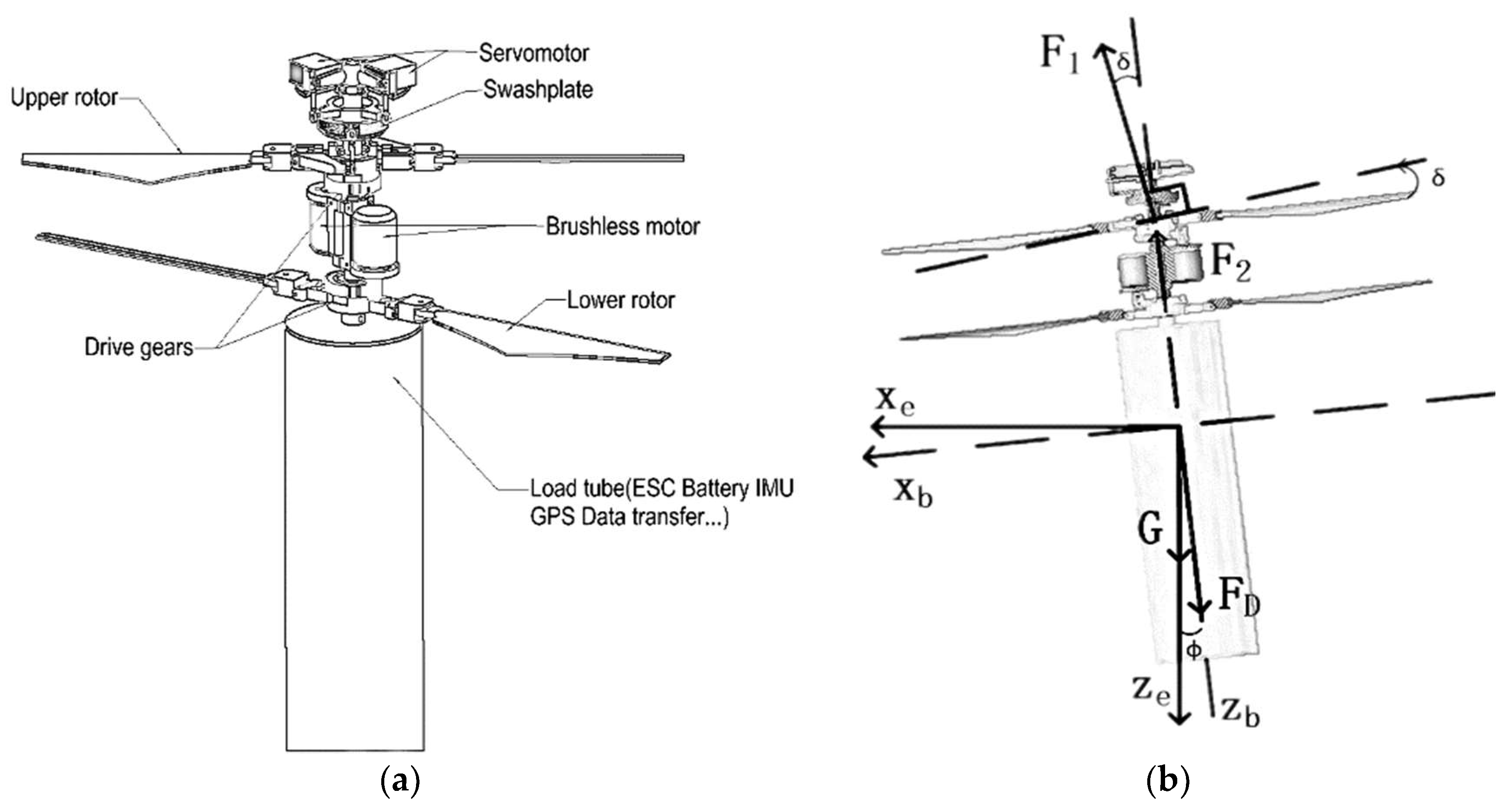
This paper is organized as follows: In Section 2, according to the self-developed coaxial vehicle, the modeling and derivation processes are given. In Section 3, the decoupling algorithm design is introduced. The controller design and stability analysis based on the fuzzy sliding mode control are described in Section 4. Finally, the simulation results and comparison with the decoupling algorithm are shown in Section 5.

2. Aircraft Longitudinal Flight Model

There is a large degree of coupling among the control inputs of the aircraft. The general method is to regard these coupling quantities as external disturbances, but this method introduces large errors. To solve this problem, we used the method of controlling the correlation coefficient of the input, by selecting the appropriate correlation coefficient so that coupling among the control inputs would be handled better.

2.1. Rotor System Modeling

In order to establish a simplified model that could both reflect the aerodynamic characteristics of a coaxial-rotor and be suitable for controller design, we first made the following assumptions: The blade was rigid, the blade root truncation effect was ignored, and the tip loss and the flapping hinge extension were assumed without considering the unsteady effect [15]. The structure design and force analysis of the coaxial-rotor are shown in Figure 1.

Based on the blade-element theory, the integral expression of the rotor pulling force and torque could be obtained:

$$\begin{array}{l}T=\frac{N_b}{2\pi }{\displaystyle {\int }_0^{2\pi }{\displaystyle {\int }_0^{R-e}\left(l{c}_v-d{s}_v\right)drd{\psi }_f}}\\ Q=\frac{N_b}{2\pi }{\displaystyle {\int }_0^{2\pi }{\displaystyle {\int }_0^{\mathrm{R}-e}\left(l{c}_v-d{s}_v\right)rdrd{\psi }_f}}\end{array}$$

(1)

where $N_b$ is the number of blades, $R$ is the radius of the rotor, $e$ is the amount of hinge extension of blade swing, ${\psi }_f$ is the local azimuth, $r$ is the local radial coordinates, $l$ and $d$ respectively are local lift and resistance, and $c_v$ and $s_v$ are the correction terms related to the aircraft and the flying environment [16]. The approximate inflow ratio of a blade-element was:

$$\lambda ={\lambda }_{in}+{\lambda }_{fs}=\frac{v_{in}}{\mathsf{\Omega }R}-\frac{v_b}{\mathsf{\Omega }R}$$

(2)

where $v_{in}$ is the induced velocity, Ω is the rotor speed, $v_b$ is the rotor speed, is the body speed, and ${\lambda }_{in}$ and ${\lambda }_{fs}$ are the inflow ratio corresponding to the induced velocity and body velocity, respectively.

To solve the problem of interference between coaxial rotors, the Pitt–Peters dynamic inflow method was used to model the induced velocity. The specific method was to connect the dynamic variation of the induced velocity with the variation of aerodynamic parameters through a first-order linear differential equation. We could then clarify the relationship between the pull coefficient and the induced velocity through integral calculation. The method was simple and in good agreement with the experimental data. The proposed model could be well applied to the simulation and controller designs. According to the dynamic inflow model, the relationship between the induced velocity and the pull coefficient was as follows:

$$M{\dot{\lambda }}_{in}+V{L}^{-1}{\lambda }_{in}=C$$

(3)

where $M$, $V$ and $L$ are the parameter matrix of inflow dynamics, respectively, ${\lambda }_{in}={\left({\lambda }_0+{\lambda }_s+{\lambda }_c\right)}^T$ represents the time-averaged, first-order horizontal, and vertical components of the induced inflow ratio. $C={\left(C_T+C_l+{\lambda }_m\right)}^T$ represents the pull torque, roll torque and pitch torque coefficients of the rotors. The interaction of the induced velocity is expressed as:

$${\lambda }_i={\lambda }_{in,i}+K_{ji}{\lambda }_{in,j}+{\lambda }_{fs}{e}_1$$

(4)

where $i$, $j$ are the upper and lower rotors and $K_{ji}$ is the parameter matrix, indicating the influence of the induced velocity between the upper and lower rotors related to the distance between the rotors, airfoil, and flight state, while $e_1={\left(\begin{array}{ccc}1& 0& 0\end{array}\right)}^T$.

Considering that the interaction of the induced velocity mainly affected the channels of total distance and heading, the induced velocity in the plane of the propeller disk was almost unaffected. Assuming that the induced velocity was uniformly distributed in the plane of the propeller disk, the average inflow ratio and the differential inflow ratio were defined respectively as:

$$\begin{array}{l}{\lambda }_a=\frac{1}{2}\left({\lambda }_u+{\lambda }_l\right)\\ {\lambda }_r=\frac{1}{2}\left({\lambda }_u-{\lambda }_l\right)\end{array}$$

(5)

From the formulas above, the pull and torque coefficients could be obtained using integral calculation ($\tau$ is the rotor flapping time constant):

$$\begin{array}{l}{C}_{Ti}=\frac{\sigma a_0}{2}\left(\frac{1}{3}{\theta }_i-\frac{1}{2}\right){\lambda }_i\\ C_{Qi}={\lambda }_i{C}_{Ti}+\frac{\sigma }{8}{C}_D\end{array}$$

(6)

So, the single rotor thrust and torque were presented:

$$\begin{array}{l}{T}_i=\rho A{\left({\mathsf{\Omega }}_{i}R\right)}^2{C}_{Ti}\\ Q_i=\rho A{\mathsf{\Omega }}_i{}^2{R}^3{C}_{Qi}\end{array}$$

(7)

where subscript $i$ represents the upper rotor (u) or the lower rotor (l), ${\theta }_i$ is the pitch, c is the chord length of the blade, $A$ is the paddle area, $a_0$ is the slope of the lift line of the airfoil, $C_D$ is the airfoil drag coefficient, $\rho$ is the air density, and $\sigma =\left(N_{b}c\right)/\left(\pi R\right)$ is the real degree of the paddle.

2.2. External Force Modeling

In the steady state of hovering, the external force of the aircraft was determined by the lift $F_1$ and $F_2$, the gravity $G$, and the aerodynamic resistance, $F_D$:

$$F=F_1+F_2+G+F_D$$

(8)

2.2.1. The Lift of the Rotor System

The lift of the designed aircraft was provided by the upper and lower rotors. Since the swash plate related to the upper rotor, the upper rotor provided both lift and lateral force, while the lower rotor only provided lift. The following could be obtained from Formulas (2) and (7):

$$\begin{array}{l}{F}_1=\rho A{\left({\mathsf{\Omega }}_{u}R\right)}^2{C}_{Tu}\cos \delta \\ F_2=\rho A{\left({\mathsf{\Omega }}_{l}R\right)}^2{C}_{Tl}\end{array}$$

(9)

2.2.2. The Gravity of Aircraft

The mass of aircraft is $m$, and the body gravity was expressed by the body coordinate system data:

$$G=mg\left[\begin{array}{c}-\sin \theta \\ \cos \theta \sin \varphi \\ \cos \theta \cos \varphi \end{array}\right]$$

(10)

2.2.3. The Aerodynamic Resistance

According to the empirical formula of aerodynamics, the resistance of the fuselage in the hovering state could be expressed as:

$$F_D=\frac{1}{2}\rho V^2{A}_{fus}{C}_{Dfus}$$

(11)

where $V$ is the relative fly-forward speed of the aircraft, $A_{fus}$ is the equivalent cross-sectional area of the body, and $C_{Dfus}$ is the resistance coefficient of the whole body.

2.3. Establishing the Longitudinal Posture Model

$$\{\begin{array}{l}-m\ddot{x}=-\left(F_1\cos \delta +F_2-F_D\right)\sin \varphi +{\epsilon }_0{F}_{1}d\sin \delta \cos \varphi \hfill \\ -m\ddot{z}=\left(F_1\cos \delta +F_2-F_D\right)\cos \varphi +{\epsilon }_0{F}_{1}d\sin \delta \sin \varphi -mg\hfill \\ I_{xx}\ddot{\varphi }=F_{1}d\sin \delta \hfill \end{array}$$

(12)

Take $x_1=-x$, $x_2=\dot{x}$, $z_1=-z$, $z_2=\dot{z}$, $u_1=\left(F_1\cos \delta +F_2-F_D\right)/m$, $u_2=\left(F_{1}d\sin \delta \right)/I_{xx}$,

$\epsilon =\frac{{\epsilon }_0{I}_{xx}}{m}$. Formula (12) [17,18] could be written as:

$$\{\begin{array}{l}{\dot{x}}_1=x_2\hfill \\ {\dot{x}}_2=-u_1\sin \varphi +\epsilon u_2\cos \varphi \hfill \\ {\dot{z}}_1=z_2\hfill \\ {\dot{z}}_2=u_1\cos \varphi +\epsilon u_2\sin \varphi -g\hfill \\ \dot{\varphi }=\phi \hfill \\ \dot{\phi }=u_2\hfill \end{array}$$

(13)

where $x_1\left(t\right)$, $z_1\left(t\right)$ and $\varphi \left(t\right)$ are the mass center and deflection angles of aircraft, $u_1$ and $u_2$ are the control inputs, $g$ is the gravitational acceleration, and ${\epsilon }_0$ represents the parasitic force of lateral displacement generated by rolling torque and ${\epsilon }_0\ne 0$ [19]. The system’s output was:

$$y\left(t\right)={\left[\begin{array}{ccc}{x}_1\left(t\right)& z_1\left(t\right)& \varphi \left(t\right)\end{array}\right]}^T$$

(14)

3. Design of the Decoupling Algorithm

Formula (13) was a strong non-linear coupling model [20]. In order to transform the model into the under-driven standard form, the following method was used to decouple the model [21,22].

3.1. Eliminate the Control Coupling of ${\dot{x}}_2$ and ${\dot{z}}_2$

In order to eliminate the control coupling of ${\dot{x}}_2$ and ${\dot{z}}_2$, the following decoupling algorithm could be designed:

$$\left[\begin{array}{l}{u}_1\\ u_2\end{array}\right]={\left[\begin{array}{cc}-\sin \varphi & \epsilon \cos \varphi \\ \cos \varphi & \epsilon \sin \varphi \end{array}\right]}^{-1}\left[\begin{array}{c}{u}_{m1}\\ u_{m2}+g\end{array}\right]$$

(15)

where $u_{m1}$ and $u_{m2}$ are the control items to be designed. Next, Formula (13) could be changed:

$$\{\begin{array}{l}{\ddot{x}}_1=u_{m1}\\ {\ddot{z}}_1=u_{m2}\\ \epsilon \ddot{\varphi }=u_{m1}\cos \varphi +\left(u_{m2}+g\right)\sin \varphi \end{array}$$

(16)

3.2. Eliminate the Coupling of $u_{m1}$ and $u_{m2}$

In order to eliminate the coupling of $u_{m1}$ and $u_{m2}$ in $\epsilon \ddot{\varphi }$, the following decoupling algorithm could be designed:

$$\{\begin{array}{l}{x}_m=x_1-\epsilon \sin \varphi \\ z_m=z_1+\epsilon \cos \varphi \\ u_{m1}=\left(u_{m3}-\epsilon {\dot{\varphi }}^2\right)\sin \varphi +\epsilon u_{m4}\cos \varphi \\ u_{m2}=-\left(u_{m3}-\epsilon {\dot{\varphi }}^2\right)\cos \varphi +\epsilon u_{m4}\sin \varphi -g\end{array}$$

(17)

where $u_{m3}$ and $u_{m4}$ are the control items to be designed, then Formula (16) could be changed:

$$\{\begin{array}{l}{\ddot{x}}_m=u_{m3}\sin \varphi \\ {\ddot{z}}_m=-u_{m3}\cos \varphi -g\\ \ddot{\varphi }=u_{m4}\end{array}$$

(18)

3.3. Eliminate the Coupling of $\sin \varphi$ and $\cos \varphi$

In order to eliminate the coupling of $\sin \varphi$ and $\cos \varphi$, the following decoupling algorithm was designed:

We took $q_1=x_m$, $q_2={\dot{q}}_1$, $q_3=z_m$, $q_4={\dot{q}}_3$, $q_5=\tan \varphi$, and $q_6={\dot{q}}_5$, and when $\varphi$ was very small, we took $\sin \varphi \approx \varphi$. Then we could obtain the following:

$${\ddot{q}}_5=\frac{u_{m4}{\cos }^2\varphi +2{\dot{\varphi }}^2{\cos }^3\varphi \sin \varphi }{{\cos }^4\varphi }$$

(19)

We took $h_1=u_{m3}\cos \varphi$, $h_2={\tan }^{″}\varphi$. Then we could get $u_{m4}=h_2{\cos }^2\varphi -2{\dot{\varphi }}^2\tan \varphi$. Now, $h_1$ and $h_2$ were the control items to be designed. Then, Formula (18) could be changed as:

$$\{\begin{array}{l}{\dot{q}}_1=q_2\\ {\dot{q}}_2=q_5{h}_1\\ {\dot{q}}_3=q_4\end{array}\begin{array}{cc}& \{\begin{array}{l}{\dot{q}}_4=-h_1-g\\ {\dot{q}}_5=q_6\\ {\dot{q}}_6=h_2\end{array}\end{array}$$

(20)

3.4. Transform the Control Model into an Under-Driven Standard Form

The under-driven standard form could be obtained:

$$\{\begin{array}{l}{\dot{y}}_1=y_2\\ {\dot{y}}_2=f_1\left(\begin{array}{ccc}{y}_1& y_2& y_3\end{array}\right)\\ {\dot{y}}_3=y_4\\ {\dot{y}}_4=f_2\left(\begin{array}{ccc}{y}_1& y_2& y_3\end{array}\right)+bh+d\end{array}$$

(21)

where $f_2\left(\begin{array}{ccc}{y}_1& y_2& y_3\end{array}\right)=\left[\begin{array}{c}-g\\ 0\end{array}\right]$, $b=\left[\begin{array}{cc}-1& 0\\ 0& 1\end{array}\right]$, $h=\left[\begin{array}{c}{h}_1\\ h_2\end{array}\right]$, and $d$ is the control disturbance. In order to make $\frac{\partial f_1\left(\begin{array}{ccc}{y}_1& y_2& y_3\end{array}\right)}{\partial y_3}$ invertible, which would be helpful for the design of the control law, we took $y_2=\left[\begin{array}{c}{q}_2+q_4{q}_5\\ {\displaystyle \int \begin{array}{l}t\\ 0\end{array}}{q}_{3}dt\end{array}\right]$, $y_1=\left[\begin{array}{l}{q}_1+{\displaystyle \int \begin{array}{l}t\\ 0\end{array}}{q}_4{q}_{5}dt\\ {\displaystyle \int \begin{array}{l}t\\ 0\end{array}}\left({\displaystyle \int \begin{array}{l}t\\ 0\end{array}}{q}_3{d}_t\right)dt\end{array}\right]$, $y_3=\left[\begin{array}{l}{q}_3\\ q_5\end{array}\right]$, $y_4=\left[\begin{array}{l}{q}_4\\ q_6\end{array}\right]$, and $f_1\left(\begin{array}{ccc}{y}_1& y_2& y_3\end{array}\right)=\left[\begin{array}{c}-g{y}_3\left(2\right)\\ y_3(1)\end{array}\right]$.

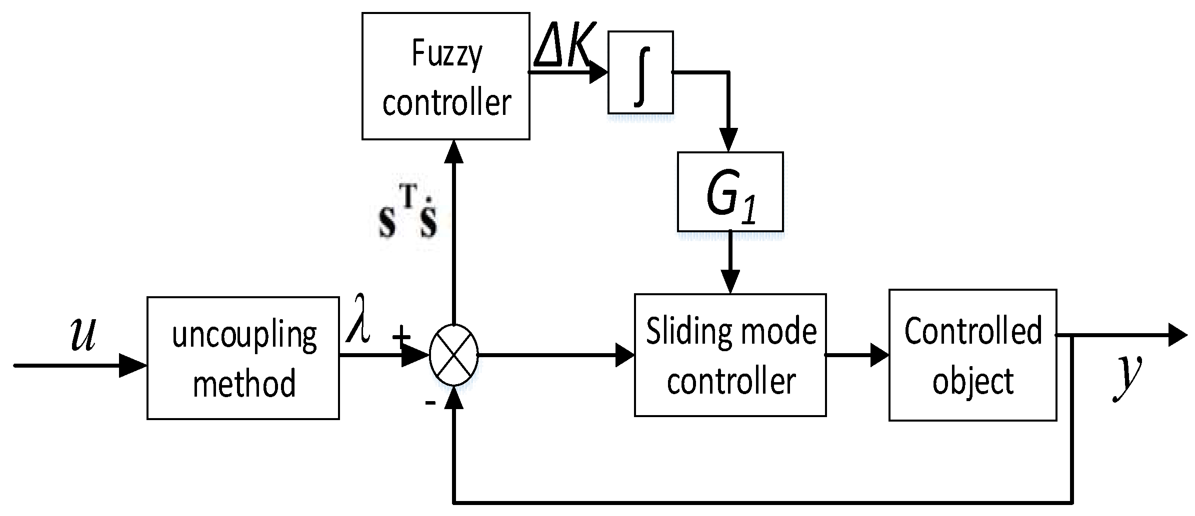
4. Design of the Controller

The structure of the controller [16] is shown in Figure 2.

4.1. Design of the Control Law

In order to design the control law for Formula (21), we took $y_{1d}$ as the reference instruction of $y_1$, and the error variables were as follows [19]:

$$\begin{array}{l}{e}_1=y_1-y_{1d},e_2=y_2-{\dot{y}}_{1d}\\ e_3=f_1-{\ddot{y}}_{1d},e_4=\frac{\partial f_1}{\partial y_3}{y}_4-y_{1d}{}^{(3)}\end{array}$$

(22)

Next, we designed the sliding surface:

$$s={\mathrm{c}}_1{e}_1+{\mathrm{c}}_2{e}_2+{\mathrm{c}}_3{e}_3+e_4$$

where $c_i>0$ and $i=1,2,3$.

When $\dot{s}=0$, we could obtain $h=u_{eq}$ and ${\mathrm{c}}_1{\dot{e}}_1+{\mathrm{c}}_2{\dot{e}}_2+{\mathrm{c}}_3{\dot{e}}_3+{\dot{e}}_4=0$.

The equivalent switch control items could thus be obtained [23]:

$$\begin{array}{l}{u}_{eq}=-{\left(\frac{\partial f_1}{\partial y_3}b\right)}^{-1}({\mathrm{c}}_1{y}_2-{\mathrm{c}}_1{\dot{y}}_{1d}\\ +{\mathrm{c}}_2{f}_1-{\mathrm{c}}_2{\ddot{y}}_{1d}+{\mathrm{c}}_3\frac{\partial f_1}{\partial y_3}{y}_4\\ -{\mathrm{c}}_3{y}_{1d}{}^{(3)}+\frac{\partial f_1}{\partial y_3}{f}_2-y_{1d}{}^{(4)})\end{array}$$

(23)

where ${\dot{y}}_1=y_2$, ${\ddot{y}}_1=f_1$, $y_1{}^{(3)}={\dot{f}}_1=\frac{\partial f_1}{\partial y_3}{y}_4$ and $y_1{}^{(4)}={\ddot{f}}_1=\frac{\partial f_1}{\partial y_3}{\dot{y}}_4$

The switching control item was then designed:

$$u_{sw1}=-{\left(\frac{\partial f_1}{\partial y_3}b\right)}^{-1}[K\left(t\right)\mathrm{sgn}\left(s\right)+\lambda s+E_1\left(t\right)]$$

(24)

where $E_1\left(t\right)$ is unknown interference. Both $E_1\left(t\right)$ and $K\left(t\right)$ will be described in more detail in Section 4.2. The control law could be designed as follows:

$$h=u_{eq}+u_{sw}$$

(25)

4.2. Stability Analysis of the Control System

Taking Formulas (23)–(25) into $\dot{s}$, the following could be obtained:

$$\begin{array}{l}\dot{s}=c_1{\dot{e}}_1+c_2{\dot{e}}_2+c_3{\dot{e}}_3+{\dot{e}}_4\\ =c_1(y_2-{\dot{y}}_{1d})+c_2(f_1-{\ddot{y}}_{1d})+c_3\left(\frac{\partial f_1}{\partial y_3}{y}_4-y_{1d}{}^{(3)}\right)\\ +\frac{d}{dt}\left[\frac{\partial f_1}{\partial y_3}\right]y_4+\frac{\partial f_1}{\partial y_3}{f}_2-y_{1d}{}^{(4)}\\ =-K\left(t\right)\mathrm{sgn}\left(s\right)-\lambda s+\frac{\partial f_1}{\partial y_3}d\end{array}$$

We took $K\left(t\right)=\alpha \overline{d}+\mathsf{\rho }$, where $\overline{d}(1)\ge \left|d\left(1\right)\right|$, $\overline{d}(2)\ge \left|d\left(2\right)\right|$, $\mathsf{\rho }\left(1\right)>0$, $\mathsf{\rho }\left(2\right)>0$, and $\alpha >0$.

We took the Lyapunov function as $V=\frac{1}{2}{s}^{T}s$, so:

$$\begin{array}{l}\dot{V}=s^T\dot{s}=s^T\left[-(\alpha \overline{d}+\mathsf{\rho })\mathrm{sgn}\left(s\right)-\lambda s+\frac{\partial f_1}{\partial y_3}d\right]\\ \hspace{1em} =-(\alpha \overline{d}+\mathsf{\rho })\Vert s\Vert -\lambda {\Vert s\Vert }^2+s^{T}E\left(t\right)\\ \hspace{1em} \le -\mathsf{\rho }\Vert s\Vert -\lambda {\Vert s\Vert }^2\le 0\end{array}$$

(26)

where the gain of the switching $K\left(t\right)$ was the cause of chattering, and the control disturbance can be expressed as $E\left(t\right)=\frac{\partial f_1}{\partial y_3}d$, which was used for ensuring that the necessary sliding mode presence conditions were met. When $s=0$, we could obtain $e_4={\mathrm{c}}_1{e}_1+{\mathrm{c}}_2{e}_2+{\mathrm{c}}_3{e}_3$. We took the following:

$$A=\left[\begin{array}{ccc}0& 1& 0\\ 0& 0& 1\\ -c_1& -c_2& -c_3\end{array}\right]$$

$A$ is the Hurwitz function, and $\lambda$ represents the Eigenvalues of $A$, $\lambda >0$.

Taking $E_1={\left[e_1\begin{array}{cc}{e}_2& e_3\end{array}\right]}^T$, the error equation of the state could be written as ${\dot{E}}_1=A{E}_1$.

Taking $Q=Q^T>0$, we could get the Lyapunov equation $A^{T}P+PA=-Q$. The solution was $P=P^T>0$. We took the Lyapunov function as the following:

$$\begin{array}{l}{\dot{V}}_1={\dot{E}}_1^{T}P{E}_1+E_1^{T}P{\dot{E}}_1={\left(A{E}_1\right)}^{T}P{E}_1+E_1^{T}P\left(A{E}_1\right)\\ =E_1^T{A}^{T}P{E}_1+E_1^{T}PA{E}_1=E_1^T\left(A^{T}P+PA\right)E_1\\ =-E_1^{T}Q{E}_1\le -{\lambda }_{\min }\left(Q\right)\left|\right|E_1|{|}_2^2\le 0\end{array}$$

where ${\lambda }_{\min }\left(Q\right)$ is the minimum eigenvalue of positive definite matrix, $Q$.

From ${\dot{V}}_1\le 0$, we could obtain: $e_1\to 0$, $e_2\to 0$, $e_2\to 0$, then $y_1\to y_{1d}$, $y_2\to y_{2d}$, and $y_3\to y_{3d}$. From the stability of the sliding mode, we could obtain $y_4\to y_{4d}$. In the end, $x\to x_d$, $z\to z_d$, and $\varphi \to {\varphi }_d$.

4.3. Establish the Fuzzy System

The condition for the existence of sliding mode was $s^T\dot{s}<0$, and when the system reached the sliding surface, it would remain on the sliding surface [24]. From Formula (26), we could see that in order to ensure that the system movement reached the gain of the sliding surface, $K\left(t\right)$ needed to be sufficient to eliminate the impact of uncertainty. Then we could ensure the existence of the sliding condition.

The idea of the fuzzy rules was represented as follows:

If $s^T\dot{s}>0$, then $K\left(t\right)$ should increase;

if $s^T\dot{s}<0$, then $K\left(t\right)$ should be reduced.

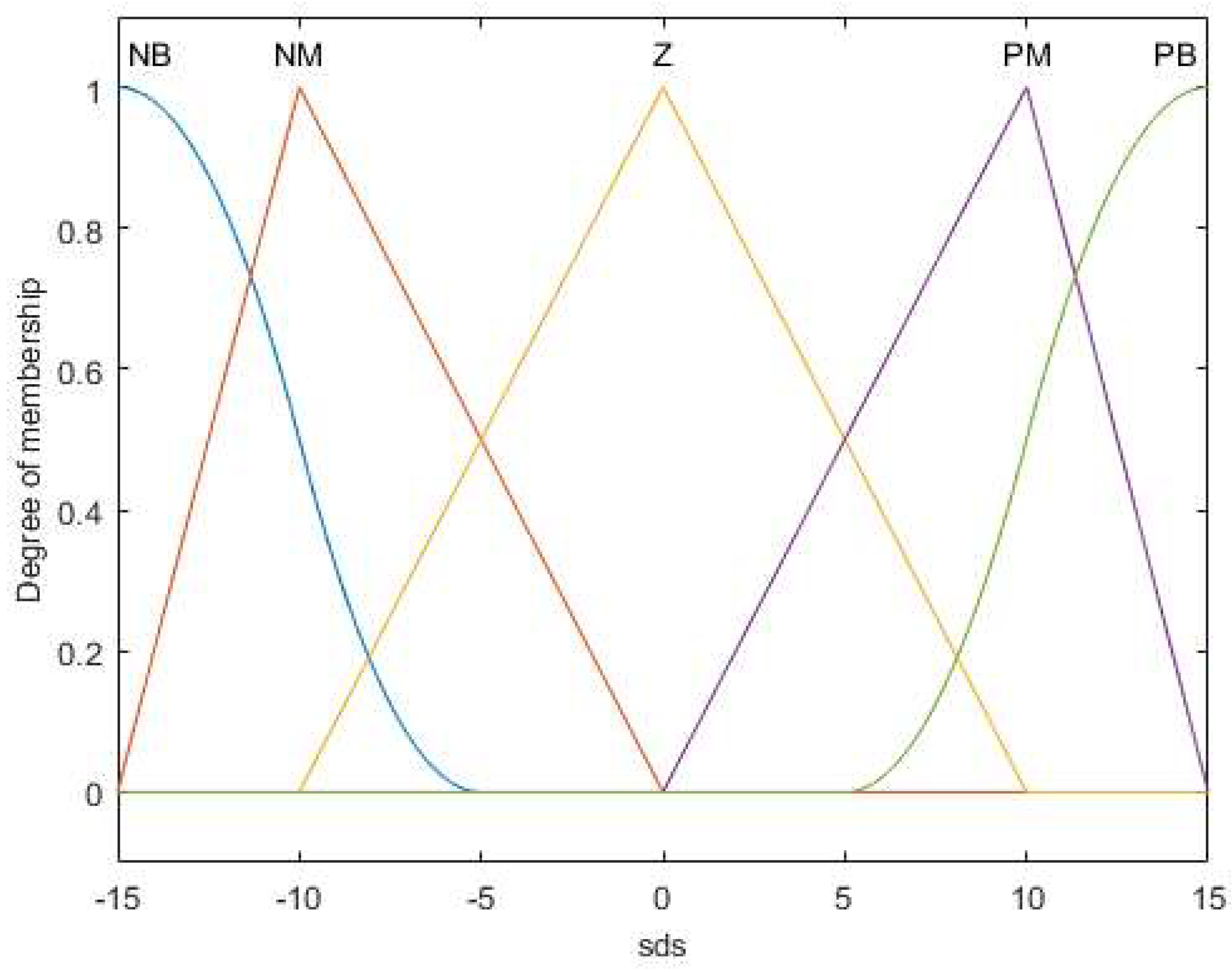
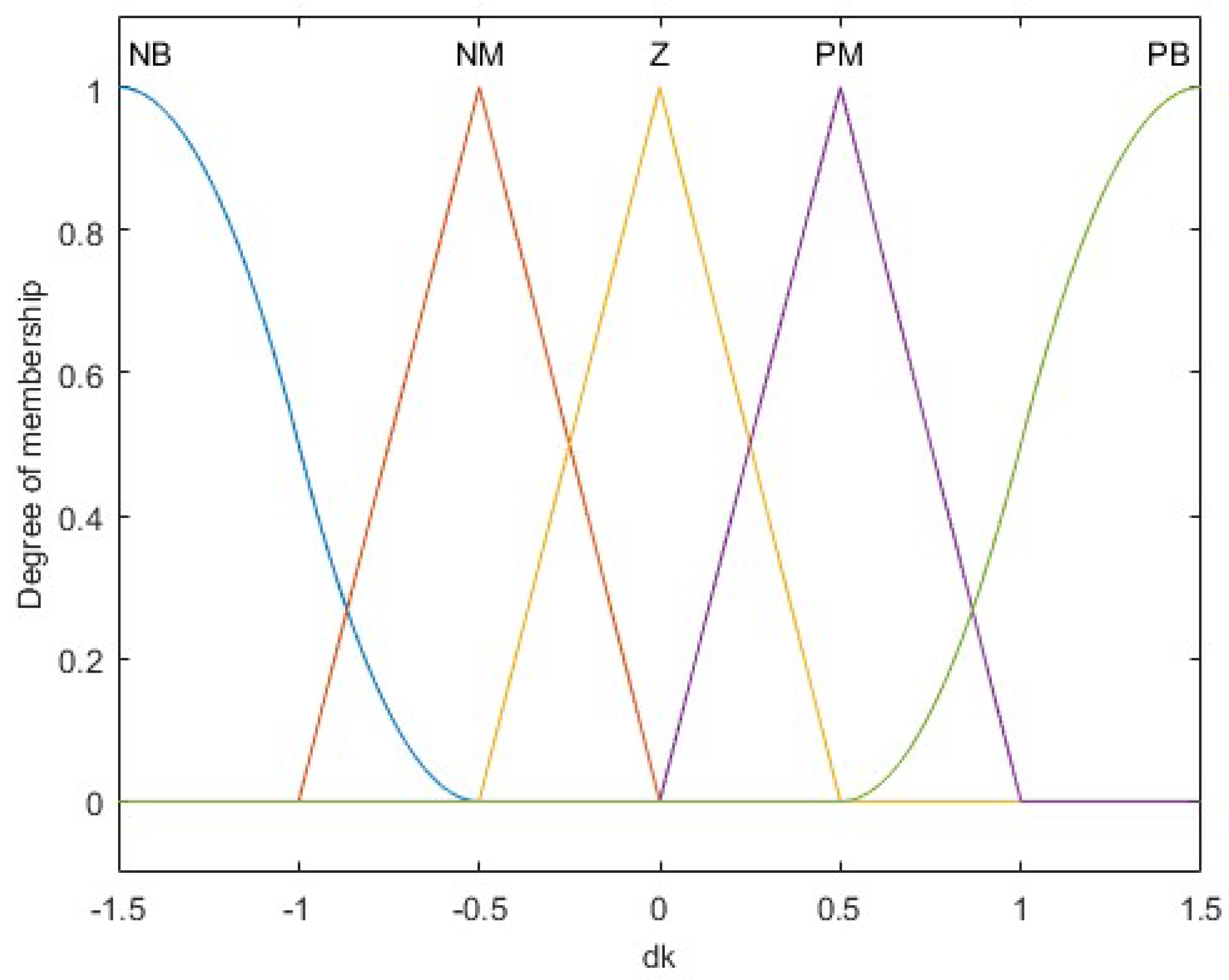
From the two types above, we could design the fuzzy system using $s^T\dot{s}$ and $\Delta K\left(t\right)$. In this system, $s^T\dot{s}$ is the input, and $\Delta K\left(t\right)$ is the output. The fuzzy sets of the system were defined as follows:

$$\begin{array}{l}{s}^T\dot{s}=\{\begin{array}{ccccc}NB& NM& ZO& PM& PB\}\end{array}\\ \Delta K=\{\begin{array}{ccccc}NB& NM& ZO& PM& PB\}\end{array}\end{array}$$

where $NB$ represents the negative big, $NM$ is the negative middle, $ZO$ is the zero, $PM$ is the positive middle, and $PB$ is the positive big. The input and output membership functions of the fuzzy system are shown in Figure 3 and Figure 4. The upper bound of $\widehat{K}\left(t\right)$ was estimated using the integral method:

$$\widehat{K}\left(t\right)=G_1{\displaystyle {\int }_0^t\Delta Kdt}$$

(27)

where $G_1$ is the proportion coefficient, determined according to experience. The control law was:

$$u_{sw2}=-{\left(\frac{\partial f_1}{\partial y_3}b\right)}^{-1}\left[\widehat{K}\left(t\right)\mathrm{sgn}\left(s\right)+\lambda s+E\left(t\right)\right]$$

(28)

5. Simulation Analysis

The physical parameters of the system model were obtained through the three-dimensional model established in the CAD software Inventor, and the model reference coefficients were calculated in accordance to the physical parameters and the modeling results. The parameters are shown in

Table 1. The main symbols and parameters.

Parameter	Description	Value	Unit
$\rho$	Local air density	$1.14$	${\mathrm{kg}/\mathrm{cm}}^2$
$g$	Local gravitational acceleration	$9.804$	${\mathrm{m}/\mathrm{s}}^2$
$R$	Rotor radius	$0.20$	$\mathrm{m}$
$A$	Area of rotor plane	$0.126$	${\mathrm{m}}^2$
$m$	Weight	$1$	$\mathrm{kg}$
$d$	Distance between upper rotor and the gravity center	$0.20$	$\mathrm{m}$
$e$	Amount of hinge extension of blade flapping	$0.05$	$\mathrm{m}$
$I_{xx}$	Inertia about x-axis	$9.16\times {10}^{-4}$	${\mathrm{kg}/\mathrm{m}}^2$
$C_{Tu}$	Trust coefficient of upper rotor	$9.42\times {10}^{-3}$	${\mathrm{rad}}^{-1}$
$C_{Tl}$	Trust coefficient of lower rotor	$6.77\times {10}^{-3}$	${\mathrm{rad}}^{-1}$
$C_{Qu}$	Torque coefficient of upper rotor	$6.14\times {10}^{-4}$	${\mathrm{rad}}^{-1}$
$C_{Ql}$	Torque coefficient of lower rotor	$6.01\times {10}^{-4}$	${\mathrm{rad}}^{-1}$

.

For the controlled Formula (13), we took $\epsilon =10$ and $g=9.8$, and set a predetermined track as $x_d=t,z_d=\sin t$ and ${\varphi }_d=0$.

In order to make A become the Hurwitz function, we took the control law parameters $c_1=27,c_2=27,c_3=9$ and $\lambda =0.10$. The initial state of the controlled system was taken as $\left[\begin{array}{cccc}5& 0& 0.5& \begin{array}{ccc}0& 0.1& 0\end{array}\end{array}\right]$. We used the control law (Formula (25)) and saturation function method, and took the thickness of the boundary layer $\Delta$ to be $0.10$.

According to the structural characteristics of the coaxial-rotor UAV, a dynamic model of the longitudinal motion was established. The dynamic model of the aircraft was then decoupled, the fuzzy control and sliding mode controls were combined, and then a fuzzy sliding mode control based on the decoupling algorithm was designed for the coaxial-rotor. The control method was then simulated by MATLAB/Simulink. The results showed that the control method could track the command signal more quickly and efficiently compared to the method of the traditional sliding mode control. It could quickly reduce the yaw attitude angle deviation and the steady-state error could reach almost zero, and with a strong self-adaptive ability, it could achieve a better control effect. The response speed, tracking accuracy, and efficiency of the system were significantly improved.

The proposed control method could improve the stability of the system, which could effectively restrain the modeling errors and external disturbances of the aircraft’s attitude system. This method had the advantages of high control precision, strong robustness, and ease of implementation in engineering. In future studies, we will focus on the design of the decoupling algorithm under the influence of more inputs and interferences, and will apply this algorithm to specific engineering practices.

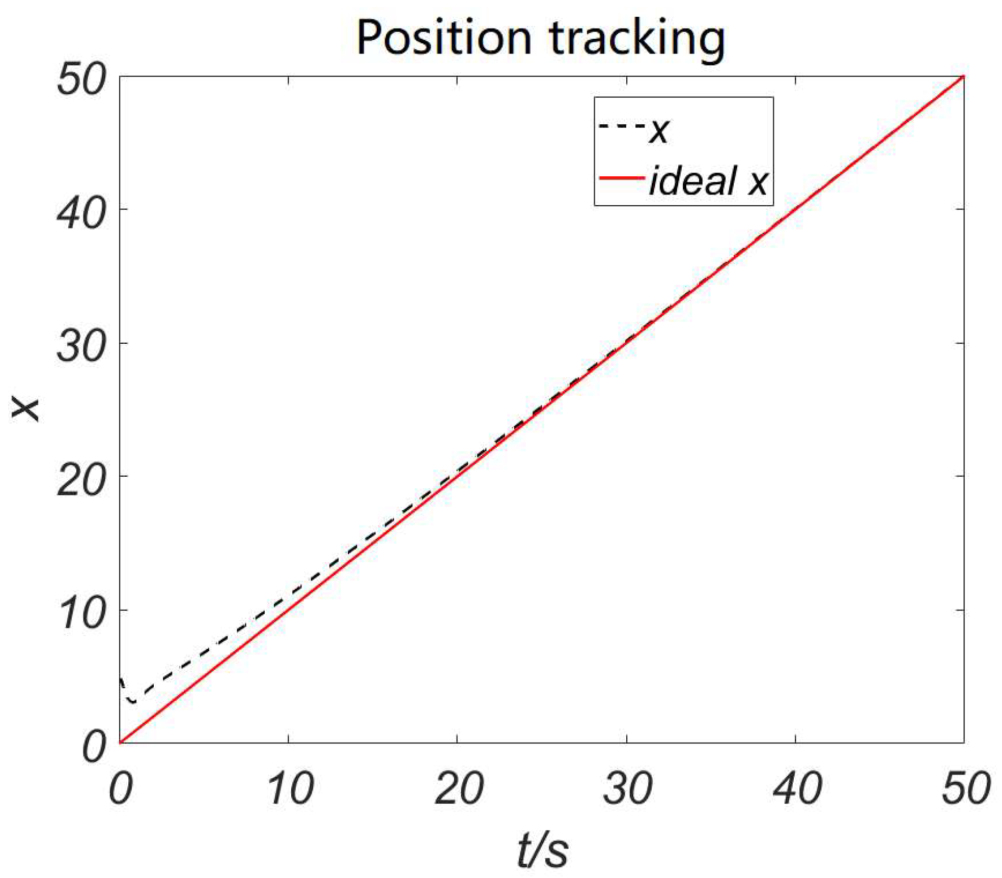
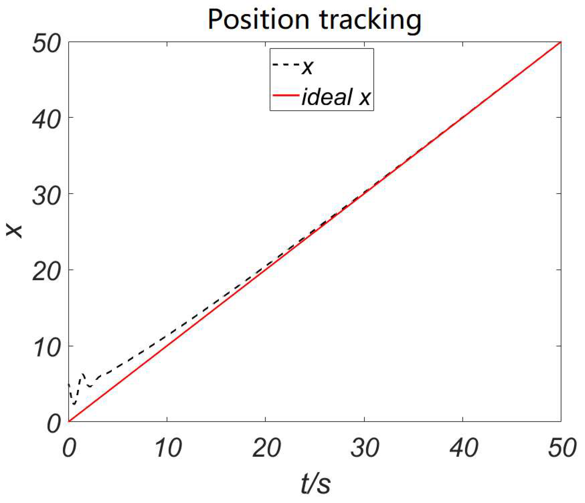
Figure 5 and Figure 6 show the performance of position tracking in the horizontal direction while the two control methods were used. The instruction given along x was a straight-line motion. The former figure indicates the position tracking with the decoupling algorithm and fuzzy control. The latter indicates the fuzzy control without the decoupling algorithm. From these figures, we could see that the performance of the control method with the decoupling algorithm and fuzzy control was faster, more accurate, and more stable than the general sliding mode control, ensuring that the aircraft would be more stable in actual movement and in improving the flight.

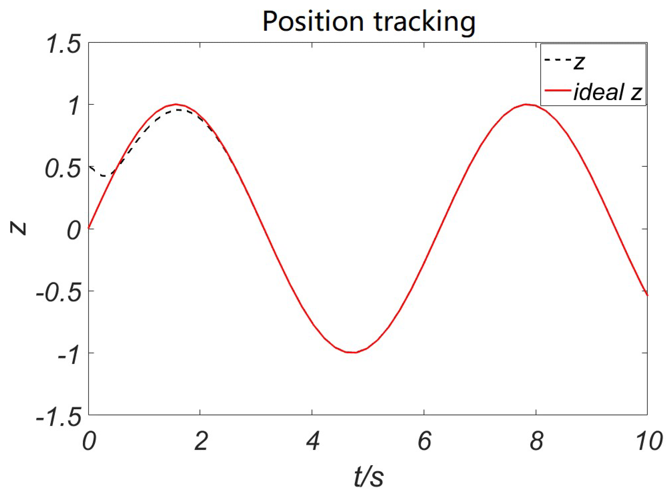
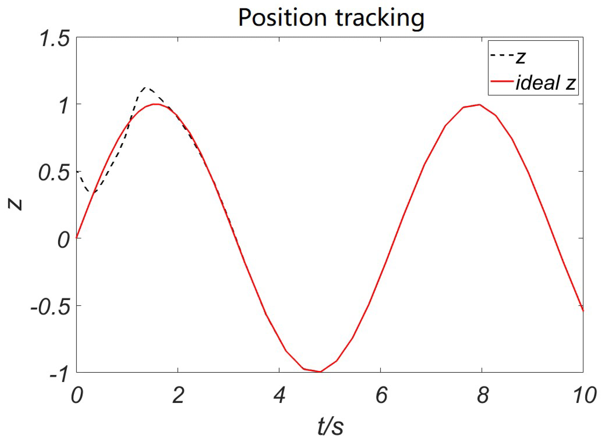
Figure 7 and Figure 8 show the performance of the position tracking in the vertical direction while the two control methods were used. The instruction given along z was a sinusoidal motion. The former figure indicates the position tracking with the decoupling algorithm and fuzzy control, and the latter indicates the general sliding mode control. From these figures we could see that the time required for the two methods to track from the initial position to the specified trajectory was almost the same, but the performance of the control method with the decoupling algorithm and fuzzy control was smoother, and the tracking error was also smaller. Thus, the flight of the aircraft would be more stable.

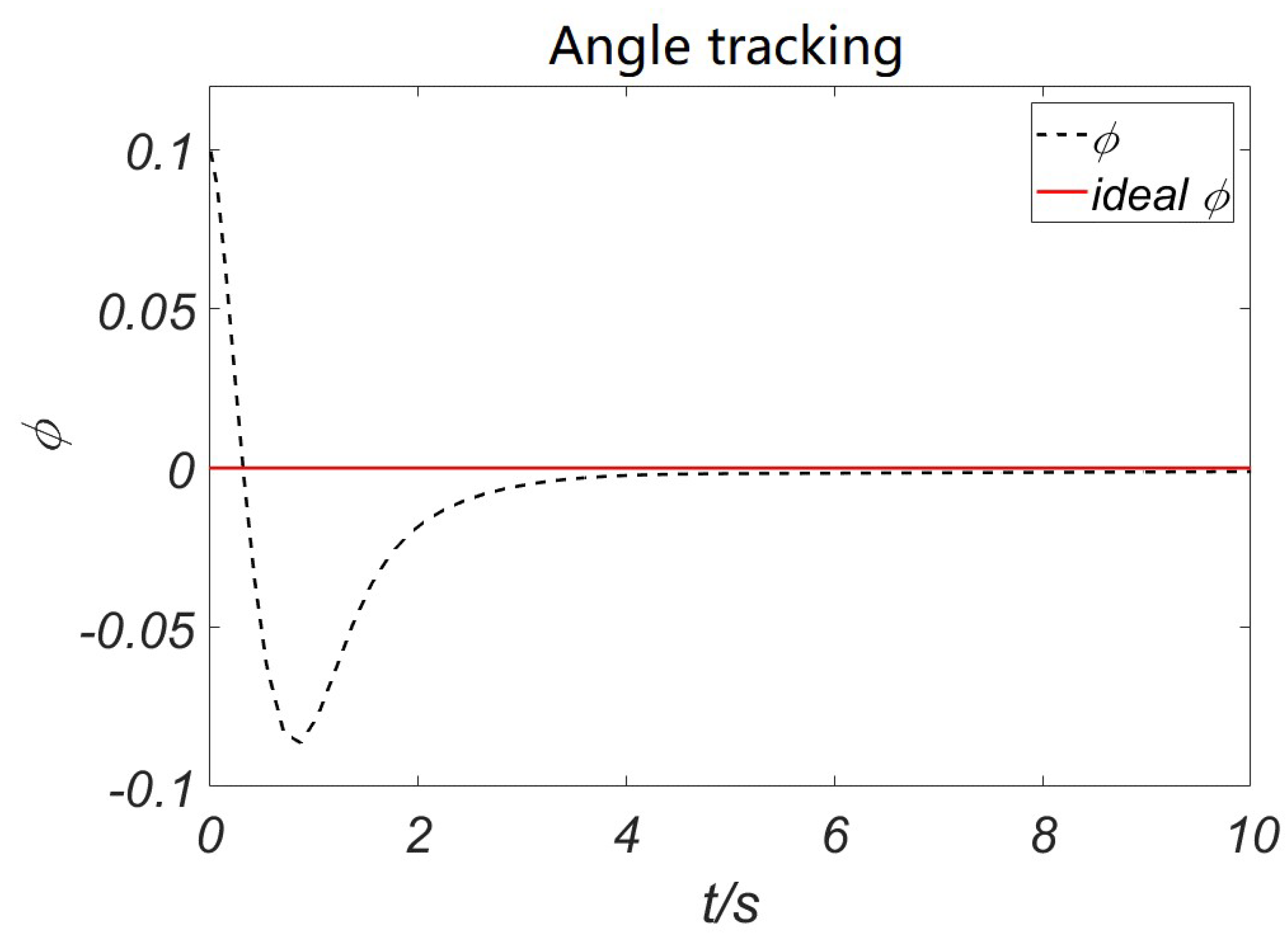
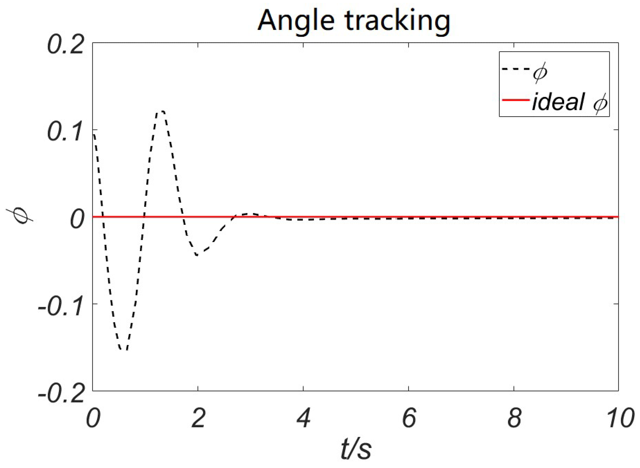
The angle tracking with the decoupling algorithm and fuzzy control are shown in Figure 9, and when compared with the angle tracking (Figure 10) without the decoupling algorithm and fuzzy control, it could be seen that in the former the tracking errors decreased while the response times were basically the same, and the movement accuracy and resistance to disturbances of the system improved. The system had better tracking performance. The impact of these disturbances, controller outputs chattering, external disturbances, and noise of the measurement were significantly reduced after the decoupling algorithm and fuzzy controller are added.

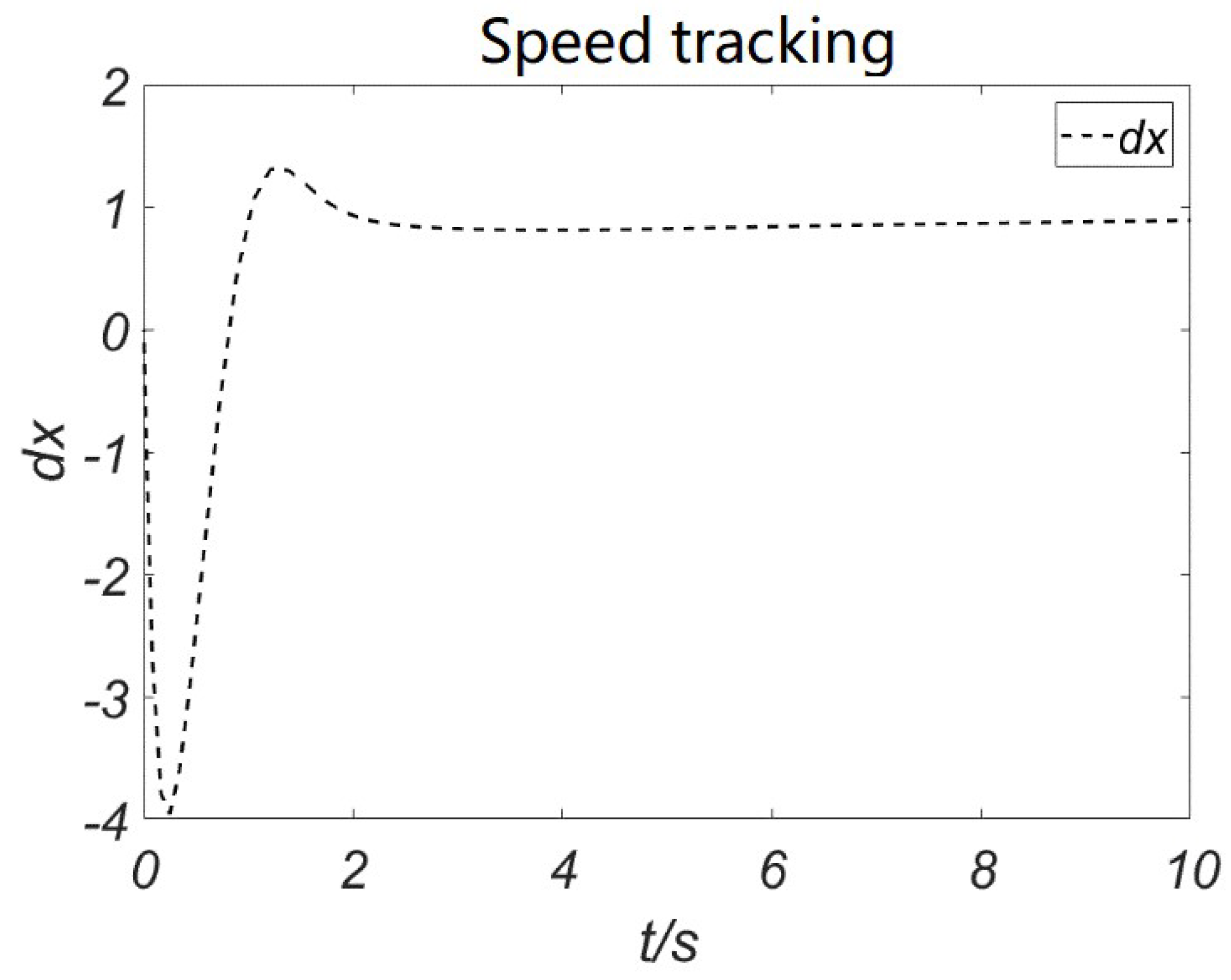
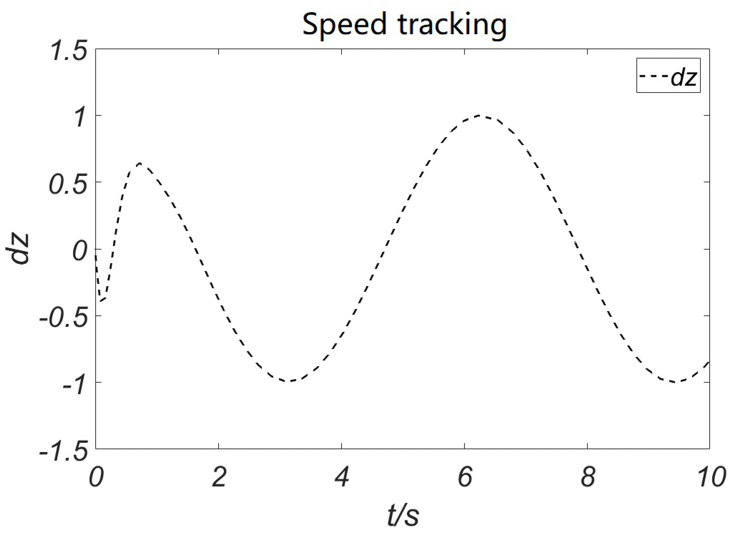
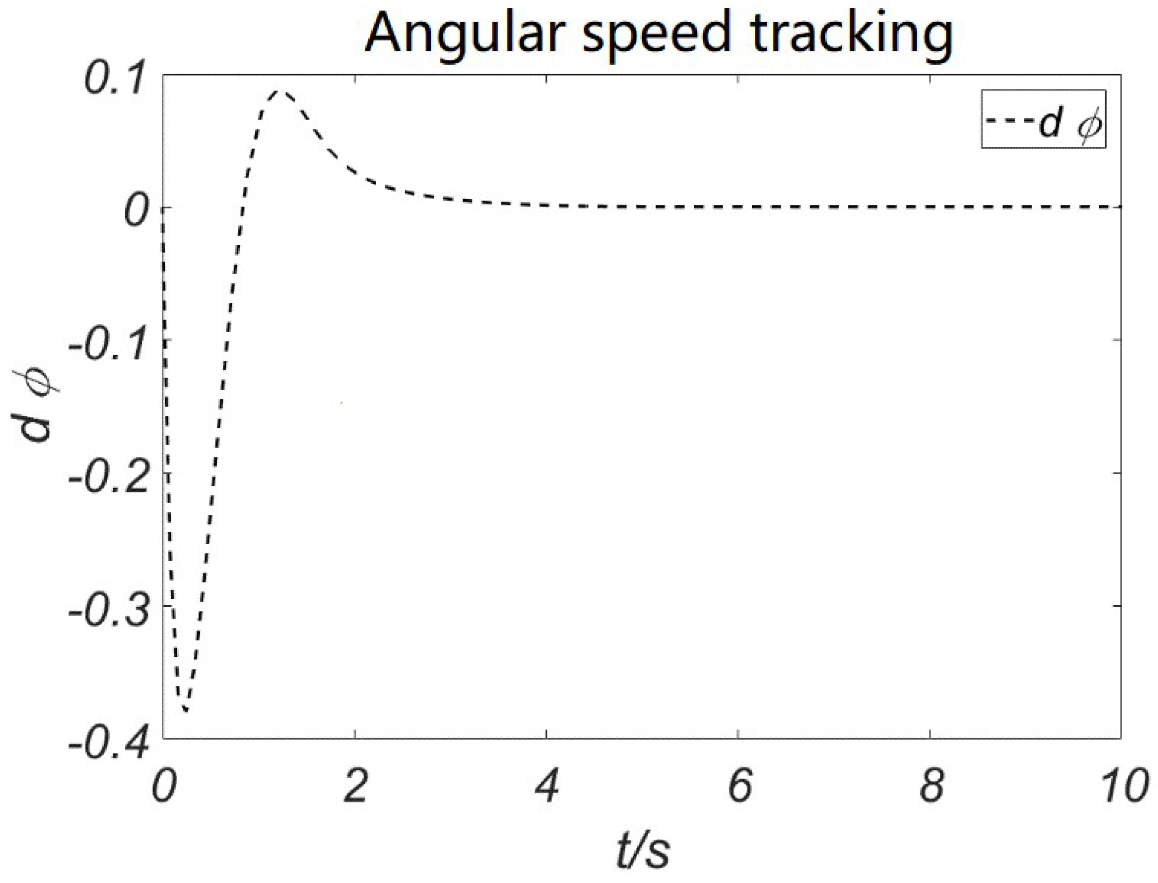
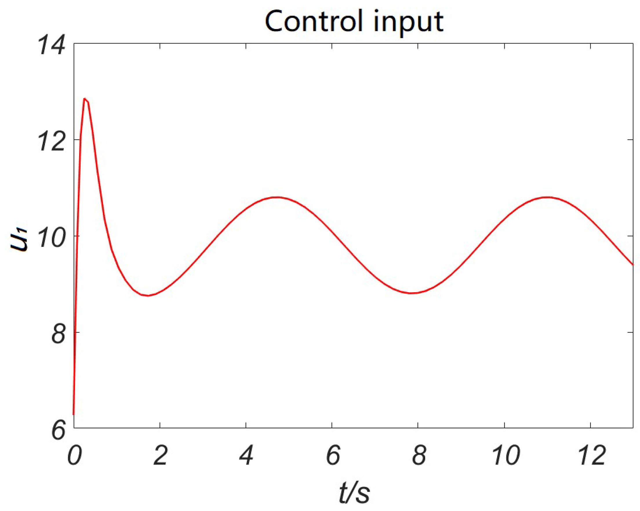
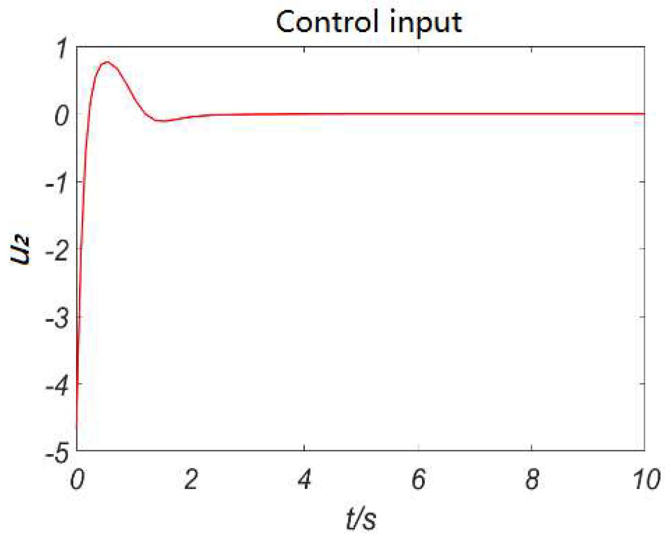
Figure 11, Figure 12 and Figure 13 show the speed tracking and angular speed tracking with the decoupling algorithm and fuzzy control. It could be seen that the change trajectory was smooth, and the time required to reach a stable state from the initial state was very short. Figure 14 and Figure 15 show the control input of the system. We could see that the control input curves were smooth and no chattering occurred. Theoretical analysis and experimental simulation results showed that the fuzzy sliding mode control based on the decoupling algorithm could improve the stability of the system, had a better self-adaptive ability, and effectively restrained the modeling errors and external disturbances of the co-rotating twin-rotor aircraft attitude system.

6. Conclusions

According to the structural characteristics of the coaxial-rotor UAV, a dynamic model of longitudinal motion was established. The dynamic model of the aircraft was then decoupled, the fuzzy control and sliding mode controls were combined, and a fuzzy sliding mode control based on the decoupling algorithm was designed for the coaxial-rotor. The control method was then simulated by MATLAB/Simulink. The results showed that the control method could track the command signal more quickly and efficiently compared to the method of the traditional sliding mode control. It could quickly reduce the yaw attitude angle deviation and the steady-state error could reach almost zero. With a strong self-adaptive ability, it could achieve a better control effect. The response speed, tracking accuracy, and efficiency of the system had been significantly improved.

The proposed control method could improve the stability of the system, which could effectively restrain the modeling errors and external disturbances of the aircraft’s attitude system. This method had the advantages of high control precision, strong robustness, and ease of implementation in engineering. In future studies, we will focus on the design of the decoupling algorithm under the influence of more inputs and interferences, and will apply this algorithm to specific engineering practices.