A Comparative Study of Different Optimization Methods for Resonance Half-Bridge Converter

Abstract

The LLC resonance half-bridge converter is one of the most popular DC-DC converters and could easily inspire researchers to design a high-efficiency and high-power-density converter. LLC resonance converters have diverse operation modes based on switching frequency and load that cause designing and optimizing procedure to vary in different modes. In this paper, different operation modes of the LLC half-bridge converter that investigate different optimization procedures are introduced. The results of applying some usual optimization methods implies that for each operation mode some specific methods are more appropriate to achieve high efficiency. To verify the results of each optimization, numerous simulations are done by Pspice and MATLAB and the efficiencies are calculated to compare them. Finally, to verify the result of optimization, the experimental results of a laboratory prototype are provided.

1. Introduction

The LLC resonant half-bridge converter is used widely in different industries and applications due to some important features such as high-power density, high efficiency, and cost effectiveness [1,2]. Zero voltage switching (ZVS) at turn-on and low turn-off current of MOSFETs in this converter makes the switching loss negligible, so switching frequency can be increased to produce a lightweight power supply for portable appliances [3].

One of the most popular methods for designing LLC resonant half-bridge converters is the first harmonic approximation (FHA) [4,5]. Though the FHA design procedure only considers the fundamental frequency harmonic and is not an accurate method to design an LLC resonant converter, the result in resonant frequency and above resonant frequency is acceptable [6]. Generally, the results of the FHA technique are considered as initial values for other optimization methods that need a starting point.

By increasing the popularity of LLC resonant converters in recent years, high-efficiency and optimum design have become more interesting for researchers. Different mathematical optimizations are applied to solve constrained or unconstrained non-linear programs with the aid of a computer. Most papers concentrate on optimizing a specific component. A study to optimize the performance of planar transformers by means of finite element analysis (FEA) is carried out in [7]. In [8] a framework for power system optimization with consideration of reliability and thermal and packaging limitation is proposed. There are other papers focusing on optimizing different aspects of converters, such as heat-sink design procedure [9], gate-drive circuitry [10] and the lowest possible inductance [11]. Generally, one of the common problems that apply to optimization procedures in the aforementioned papers is that of time-consumption, because these approaches are based on an iterative procedure involving the trial of a wide range of parameters.

A comprehensive study to achieve high conversion efficiency for LLC series resonant converters with the development of numerical computational techniques by using non-linear programming to solve the steady-state equations of converter is done in [12]. In the aforementioned paper, a mode solver by using numerical procedure is proposed to predict LLC resonant behavior at different modes. However, there are some other methods that have different approaches to find the optimum results; optimal design based on peak gain placement is presented in [13]. This method maximizes efficiency while satisfying the gain requirement for the specified input voltage range, and by following this approach the converter can minimize the conduction loss.

All applied proposed procedures to optimize the resonant converter efficiency involve different operation modes; however, in discontinuous conduction mode (DCM), solving the LLC operation mode equations involves transcendental equations, which makes it difficult to induce an explicit expression of DC characteristics. Meanwhile continuous conduction mode (CCM) operation has a closed-form solution. Therefore, in this paper, different optimization procedures are applied to different operation modes to understand which method is most appropriate for different modes for achieving high efficiency. The applied optimizer procedures in this paper are Augmented LAGrangian (ALAG) penalty function technique, Least Squares Quadratic (LSQ), modified LSQ, and Monte Carlo optimization.

In this paper, after discussing different operation modes of LLC resonant converters, in Section 3 a design procedure by FHA technique is investigated to determine the initial values for other optimizers. In Section 4, the operational procedures of optimization methods are elaborated, and power-loss equations for the components of LLC resonant converters are discussed in Section 5. The simulation results are studied in Section 6 show which optimization methods lead to achieving high efficiency in LLC resonant converter. Finally, the experimental results of a real prototype are provided in Section 7 to verify the optimization methods and obtain maximum efficiency.

2. Operating Different Modes of LLC Resonant Converters

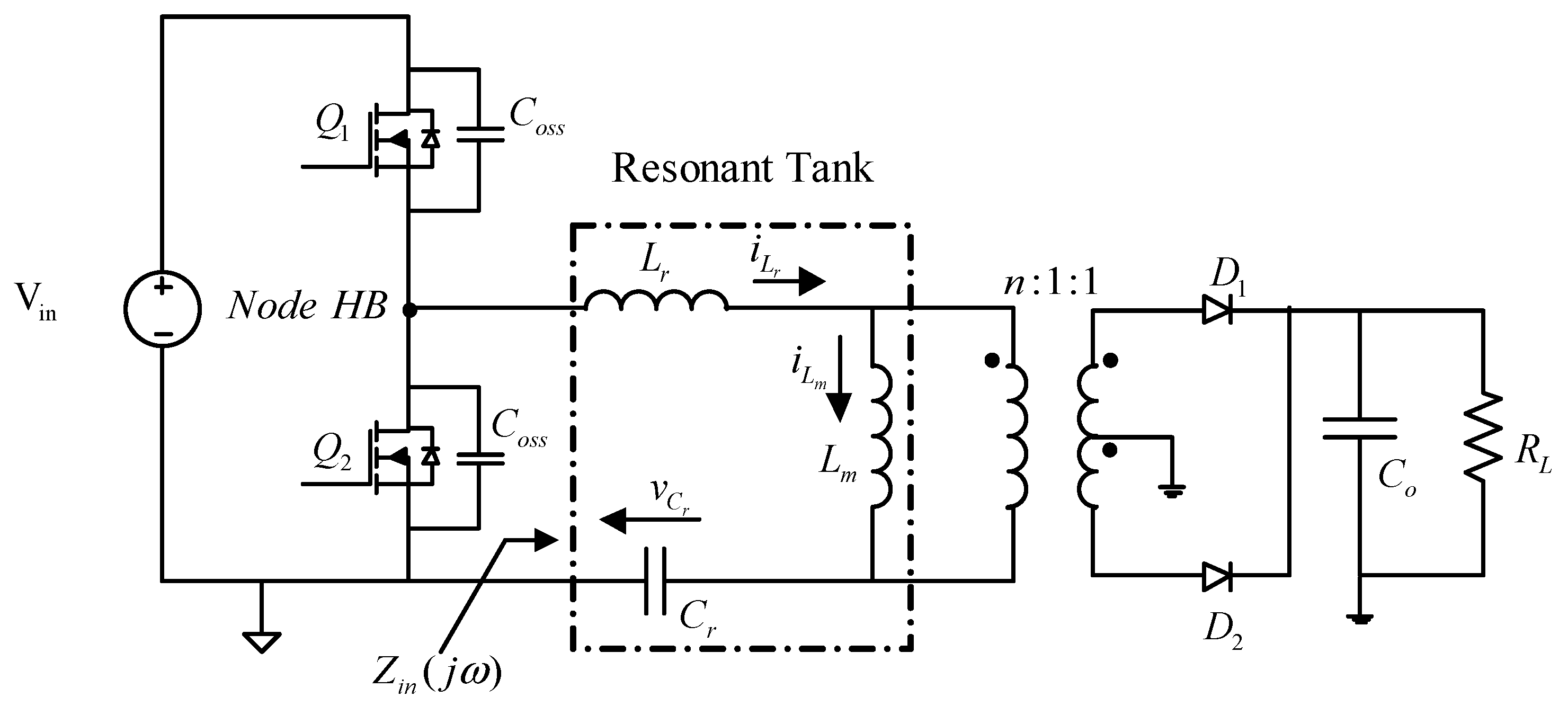
The LLC resonant half-bridge converter topology is shown in Figure 1. In this topology there are three reactive elements at the resonant tank, including two inductors and one capacitor. Consequently, there are two resonant frequencies in this converter f_r1 and f_r2:

$$f_{r1}=\frac{1}{2\pi \sqrt{L_r{C}_r}},$$

(1)

$$f_{r2}=\frac{1}{2\pi \sqrt{(L_r+L_m)C_r}},$$

(2)

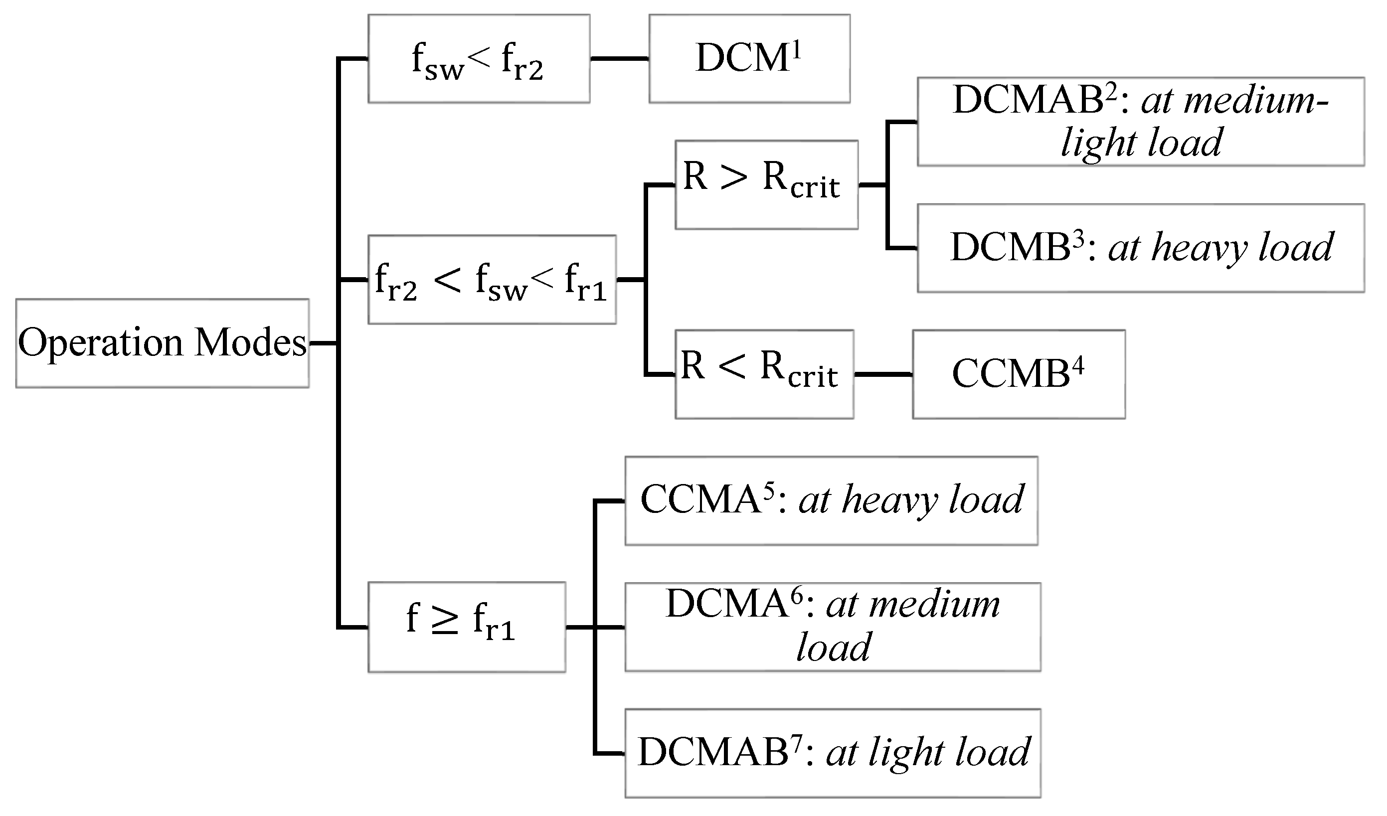
where L_r, L_m, and C_r are resonant inductor, magnetizing inductor, and resonant capacitor, respectively, and f_r1 usually considers as resonant frequency (f_r). Depending on the switching frequency and load, the converter operates in different modes. Although all the operation modes cannot be practical in this converter due to MOSFET failure in capacitive mode [14], as a general classification it is possible to illustrate the diverse operation modes as shown in Figure 2, where f_sw is the switching frequency, and R_crit is a critical value that determine the input impedance of resonant tank (Z_in(jω)) is inductive (R_L > R_crit) or capacitive (R_L < R_crit), R_crit can be stated as $R_{crit}=\sqrt{Z_{o1}.Z_{o2}}$, where Z_o1 and Z_o2 are resonant tank impedances with the source input short-circuited and open-circuited, respectively [15].

3. LLC Resonant Half-Bridge Converter Design Procedure by FHA Technique

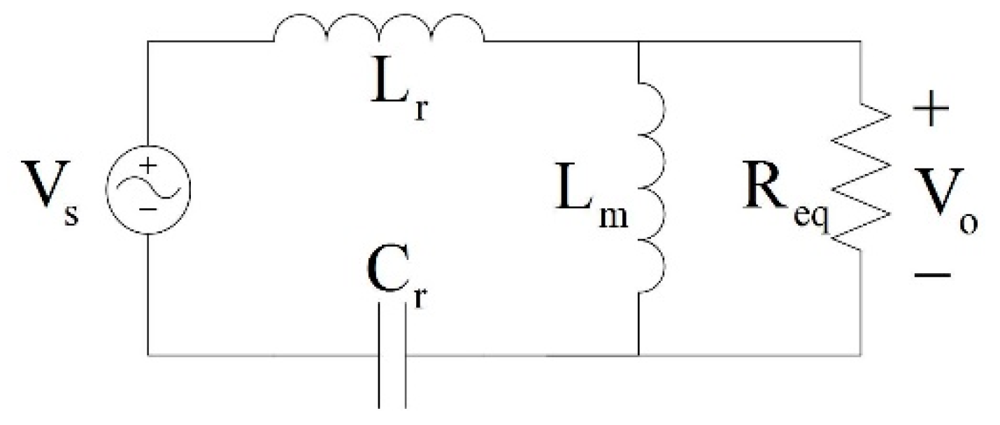
Figure 3 shows the equivalent circuit of an LLC resonant half-bridge converter at the half period in the continuous conduction mode above resonant frequency (CCMA) operation. This operation mode, as a popular mode in LLC resonant converters, can provide ZVS conditions for MOSFETs of the half-bridge converter; thus, the design procedure considers ZVS constraints. By considering the equivalent circuit voltage gain, the following equation can be obtained:

$$M=\frac{V_o}{V_s}=\frac{1}{(1+\lambda -\frac{\lambda }{f_n})+j{Q}_s(f_n-\frac{1}{f_n})},$$

(3)

where λ = L_r/L_m is the inductance ratio, fn = fsw/fr is the normalized frequency, Q_s = Z_s/R_eq is the quality factor, $Z_s=\sqrt{L_r/C_r}$ is the characteristic impedance, $R_{eq}=8n^2{V}_o^2/{\pi }^2{P}_o$ is the effective resistive load that is transferred to the primary side of transformer, where n is the turn ratio of transformer, V_o is the output voltage, and P_o is output power. Although V_s is a square wave, in this calculation only the first harmonic of its Fourier is considered.

Table 1. Procedure of LLC resonant half-bridge converter design [14].

Steps	Comments	Equations
Step 1	Calculating transformer turn ratio	$n=\frac{1}{2}\frac{V_{dc.nom}}{V_{out}}$
Step 2	Calculating max. & min. voltage gain	$M_{\max }=2n\frac{V_{out}}{V_{dc.\min }},M_{\min }=2n\frac{V_{out}}{V_{dc.\max }}$
Step 3	Calculating max. normalize frequency	$f_{n.\max }=\frac{f_{\max }}{f_r}$
Step 4	Calculating effective load resistance transfer to the primary side of transformer	${\mathrm{R}}_{\mathrm{eq}}=\frac{8}{{\mathsf{\pi }}^2}{\mathrm{n}}^2\frac{{\mathrm{V}}_{\mathrm{o}}^2}{{\mathrm{P}}_{\mathrm{o}}}$
Step 5	Calculating inductance ratio	$\lambda =\frac{1-M_{\min }}{M_{\min }}\frac{f_{n.\max }^2}{f_{n.\max }^2-1}$
Step 6	Calculating the max Q to work at ZVS region at min. input voltage and full-load condition	$Q_{\max }=\frac{\lambda }{M_{\max }}\sqrt{\frac{1}{\lambda }+\frac{M_{\max }^2}{M_{\max }^2-1}}$ $Q_{ZVS.1}=0.95\times Q_{\max }$
Step 7	Calculating the max. Q to work at ZVS region at no load condition and max. input voltage	${\mathrm{Q}}_{\mathrm{ZVS}.2}=\frac{2}{\mathsf{\pi }}\frac{\mathsf{\lambda }.{\mathrm{f}}_{\mathrm{n}.\max }}{(\mathsf{\lambda }+1).{\mathrm{f}}_{\mathrm{n}.\max }^2-\mathsf{\lambda }}\frac{{\mathrm{T}}_{\mathrm{D}}}{{\mathrm{R}}_{\mathrm{eq}}{\mathrm{C}}_{\mathrm{ZVS}}}$
Step 8	Selecting max. Q for ZVS in the whole operation range	$Q_{ZVS}\le \min \left\{Q_{ZVS.1},Q_{ZVS.2}\right\}$
Step 9	Calculating the min. operation frequency at full load and min. input voltage	$f_{\min }=f_r\sqrt{\frac{1}{1+\frac{1}{\lambda }(1-\frac{1}{M_{\max }^{1+{(\frac{Q_{ZVS}}{Q_{\max }})}^4}}}}$
Step 10	Calculating the value of resonant tank’s component	${\mathrm{Z}}_{\mathrm{o}}={\mathrm{Q}}_{\mathrm{ZVS}}.{\mathrm{R}}_{\mathrm{eq}},{\mathrm{C}}_{\mathrm{r}}=\frac{1}{2\mathsf{\pi }.{\mathrm{f}}_{\mathrm{r}}{\mathrm{Z}}_{\mathrm{o}}},{\mathrm{L}}_{\mathrm{r}}=\frac{{\mathrm{Z}}_{\mathrm{o}}}{2\mathsf{\pi }.{\mathrm{f}}_{\mathrm{r}}},{\mathrm{L}}_{\mathrm{m}}=\frac{{\mathrm{L}}_{\mathrm{r}}}{\mathsf{\lambda }}$

shows the procedure of the LLC resonant half-bridge converter design. Step 1 determines the turn ratio of the transformer by considering the nominal input voltage. Minimum and maximum voltage gain can be calculated by using Equation (3) in step 2. Steps 3 and 4 calculate the maximum normalized frequency and effective load resistance transfer to the primary side of the transformer, respectively. Also, by considering Equation (3), inductance ratio can be obtained; step 5 shows this value.

Steps 6, 7, and 8 guarantee the ZVS constraints of primary MOSFETs at whole range load variations, where C_ZVS = 2C_OSS+C_stray (C_OSS and C_stray are, respectively, the effective drain-source capacitance of the power MOSFETs and the total stray capacitance present across the resonant tank impedance at node HB). The converter could work properly at V_dc.min and minimum frequency, and at V_dc.max and maximum frequency. To find a minimum operating frequency in the ZVS operation mode, the converter should be analyzed in full-load and minimum input voltage conditions. Step 9 represents an approximate equation to find a minimum frequency [14]. Finally, in step 10, reactive elements of the resonant tank are calculated.

4. Introducing Optimization Methods

To achieve a high-efficiency converter, it is essential to consider a proper optimizer to determine the best values for different components of the converter. Generally, to achieve a high-efficiency converter, an optimization process tries to reduce the losses. Since the LLC resonant converter has non-linear behavior mostly in different modes, closed-form solutions are impossible to apply for solving equations. In this work, four usual optimization methods that can deal with non-linear equations are presented. The main aim of this paper is to determine proper optimization for each operation mode of the LLC resonant converter.

4.1. The Lagrangian Method

The Lagrangian method is one the most common mathematical solutions to find the extreme values of a function [16,17,18]. However, in our problem, of optimizing the efficiency by reducing the losses, the Lagrangian method tries to find a minimum feasible value by solving the optimization problem with linear and non-linear constraints. A complete optimization problem solved by the Lagrangian method can be defined as:

$$\min f(x_1,x_2,\dots ,x_n)=\min f(x),$$

(4)

$$subjectto\{\begin{array}{ll}{g}_i(x_1,x_2,\dots ,x_n)=0& i=1,2,\dots ,k\\ h_j(x_1,x_2,\dots ,x_n)\le 0& j=1,2,\dots ,m\\ A_{eq}(x_1,x_2,\dots ,x_n)=b_{eq}& \\ A(x_1,x_2,\dots ,x_n)\le b& \\ lb\le x_n\le ub& \end{array}$$

To solve this optimization problem by the Lagrangian method, the Lagrangian is defined as:

$$L(x,{\lambda }_i,{\mu }_j)=f(x)+{\displaystyle \sum _{i=1}^k{\lambda }_i{g}_i+{\displaystyle \sum _{j=1}^m{\mu }_j{h}_j}},$$

(5)

Finally, the optimization problem can be defined as:

$$\min L(x,{\lambda }_i,{\mu }_j),$$

(6)

In general, the Lagrangian is the sum of the original objective function and a term that involves the functional constraint and Lagrange multipliers such as ${\lambda }_i$ and ${\mu }_j$. In Equation (4), g_i is equality constraints, h_i is non-linear inequality constraints, m is the total number of non-linear constraints, k is the number of non-linear inequality constraints, A_eq and b_eq are linear equalities, A and b are linear inequalities, lb is the lower boundary and ub is the upper boundary of variable x. In addition, f(x₁,x₂,… ,x_n) is the sum of loss equations of all components in the LLC resonant converter. Therefore, finding the accurate loss model for each component is very important in the final result of the optimization.

4.2. Least Squares Quadratic (LSQ) Optimization

The LSQ problem is based on iteratively calculating to meet some specific goals by adjusting different parameters [19]. The LSQ problem tries to minimize the total error:

$$\min E=\sqrt{{\displaystyle \sum _{i=1}^n{e}_i}},$$

(7)

where E is the total error and e_i is the error of each parameter determined in the goal function. Therefore, in the LSQ method, the measurement goal is regularly compared with the goal to minimize the difference between these two values. Initial values play an important role in the LSQ optimizer. If the initial value will be close to a local minimum, it may not be an optimal solution. To find the global minimum solution, it may require extending the search space of starting points.

4.3. Modified LSQ Optimization

Modified LSQ is generally similar to the LSQ optimization [20]. However, it runs faster than LSQ for the sake of reducing the number of incremental adjustments into the goal. This optimizer can consider both constrained and unconstrained minimization problems. To implement the optimization procedure, two general algorithms are supposed to apply: least squares and minimization. Modified LSQ uses least squares algorithm when optimizing for more than one goal, then tries to reduce the sum of the squares to zero. By increasing goals, it will be more complicated for the optimizer to reduce the sum of the squares to zero.

4.4. Monte Carlo Optimization

Monte Carlo optimization is one of the stochastic optimization methods that generates and uses random variables [21,22]. This optimization method relies on iteration as well as LSQ and modified LSQ. However, by using random values in the Monte Carlo method to solve the problem, the probability of getting stuck in an unacceptable local minimum is reduced. In this method, the initial values for the variables are not essential, but a domain of possible inputs need to be defined. Thus, a sample of a probability distribution for each variable produces numerous possible outputs. Generally, the Monte Carlo method follows the following steps:

• Determine the statistical properties of possible inputs;
• Generate many sets of possible inputs which follows the above properties;
• Perform a deterministic calculation with these sets; and
• Analyze statistically the results.

5. Power-Loss Calculation

Table 2. Power-loss equations of LLC resonant half-bridge converter [12,23].

Components	Loss Characteristic		Power-Loss Equations
Half-Bridge MOSFETs	Conductive Loss		$P_{con}=R_{ds}.I_{sw(rms)}^2$
	Switching Loss	At turn-on	0
		At turn-off	$P_{sw\_OFF}=\frac{{(I_{R0}.T_f)}^2}{12.C_{HB}}.f_{sw}$
	Driving Gate Loss	At turn-on	$P_{g\_ON}=\frac{1}{2}.\frac{V_{GS}^2}{V_{GS}-V_M}\left[Q_g-(Q_{gs}+Q_{gd})\right].f_{sw}$
		At turn-off	$P_{g\_OFF}=\frac{1}{2.(V_{GS}-V_M)}\left[(V_{GS}^2+V_M^2)(Q_g-Q_{gd})-V_{GS}(V_{GS}+V_M)Q_{gs}\right].f_{sw}$
Transformer	Copper Loss		$P_{cu\_Trans}=R_{AC}.I_{RMS}^2$
	Core Loss		$P_{core}=V_e.k.f_s^{{\alpha }_{core}}.\Delta B_m^{{\beta }_{core}}$
Secondary rectifier diodes	Conductive Loss of Vf		$P_{V_f}=V_f.I_{dc.\sec }$
	Conductive Loss of rf		$P_{r_f}=r_f.I_{dc.\sec }^2$
Capacitors Loss	Input capacitance		$P{}_C=R_{ESR}.I_{RMS}^2$
	Output capacitance
	Resonant capacitance

shows power-loss equations of each component using an LLC resonant converter. Since the switches usually turn on under ZVS condition, switching losses at turn-on can be neglected. In [12,23] the power-loss equations are elaborated specifically. The voltage and current of LLC resonant converters in different operation modes are presented in [12]; these voltage and currents are essential for loss calculation.

To calculate the conductive loss of switches, R_ds represents the drain-source on-state resistance, and I_sw(rms) is the RMS value of switch current. Also, I_R0 is the current of resonant tank at half period, which can be stated as:

$$I_{R0}=i_{L_r}(\frac{T_{sw}}{2}),$$

(8)

Moreover, CHB is considered to be a capacitor at node HB that involves the sum of C_OSS of MOSFETs and stray capacitance. T_f is the time that the current of each switch takes to become zero. To calculate the driving gate losses, Q_g, Q_gs, and Q_gd indicate total gate charge, gate-source charge, and gate-drain charge of the switch, respectively. Also, V_GS is the voltage level of the driving signal, and V_M is a plateau voltage value that lets MOSFET carry the specified current.

Furthermore, to compute the copper loss of transformer, AC resistance of wire (R_AC) and the RMS values of the primary and secondary side of the transformer (I_RMS) are necessary. The volume of transformer core (V_e), transformer flux density (B_m), and k, ${\alpha }_{core}$, ${\beta }_{core}$ that are Steinmetz coefficients, are essential for core loss calculation as well. Rectifier diodes losses comprise conduction losses associated with forward voltage (V_f) and dynamic resistance (r_f). Finally, capacitor loss is calculated by considering the equivalent series resistance (R_ESR) and the RMS value of each capacitor current.

6. Simulation Results

The introduced optimization methods apply to different operation modes of the LLC resonant converter to obtaining a high-efficiency converter. In this paper, to perform the optimization procedures, different optimization engines in Pspice and solvers in MATLAB are employed. The solvers such as “fsolve” to solve the non-linear equation problem, and “fmincon” to find the minimum constrained non-linear multivariable function are used as the Lagrangian optimization method. In addition, the LSQ, modified LSQ and Monte Carlo optimizer engines in Pspice are used to employ an optimize LLC resonant converter.

To compare the results of different optimization methods, the same conditions such as input and output voltage, load condition, design variables, and initial values for optimizers are provided. Consequently, design variables will be computed by applying different optimization methods, and power loss of components are calculated to find out the minimum power loss.

The optimization procedures consider the switching frequency, resonant inductance, magnetizing inductance of transformer, resonant capacitance, and turn ratio of the transformer as design variables to find the optimum values. The following vector shows these design variables:

$$x=[f_{sw},L_r,L_m,C_r,n],$$

(9)

Moreover, the lower and upper boundary of each variable is defined in

Table 3. Load condition, constraints and switching frequency range.

Variables	Lower Boundary	Upper Boundary	Operation Mode	Load Condition ${\mathit{V}}_{\mathit{o}\mathit{u}\mathit{t}}(\mathit{V})\&{\mathit{I}}_{\mathit{o}\mathit{u}\mathit{t}}(\mathit{A})$	Switching Frequency
$L_r$	$30\mathsf{\mu }\mathrm{H}$	$250\mathsf{\mu }\mathrm{H}$	DCMB	$V_{out}=18,I_{out}=8.44$	$69\mathrm{kHz}<f_{sw}<410\mathrm{kHz}$
$L_m$	$30\mathsf{\mu }\mathrm{H}$	$800\mathsf{\mu }\mathrm{H}$	DCMAB	$V_{out}=60,I_{out}=2.53$	$69\mathrm{kHz}<f_{sw}<410\mathrm{kHz}$
$C_r$	$5\mathrm{nF}$	$100\mathrm{nF}$	CCMA	$V_{out}=20,I_{out}=7.6$	$31\mathrm{kHz}<f_{sw}<410\mathrm{kHz}$
$n$	$1\mathrm{turn}$	$25\mathrm{turns}$	DCMA	$V_{out}=40,I_{out}=3.8$	$31\mathrm{kHz}<f_{sw}<410\mathrm{kHz}$

to obtain the possible components’ values. Finally, to find the optimum values for design variables, the objective function P_loss(x), i.e., the sum of the power-loss equation of each component, is minimized by considering the defined constraints:

$$\min P_{loss}(x),$$

(10)

To solve the problem with the Lagrangian method, the “fmincon(x)” solver of the MATLAB optimization toolbox is employed. The “fmincon(x)” tries to find a constrained minimum of a function of several variables at an initial estimate. The starting points are very important for the solver to converge the problem, and to find the feasible points.

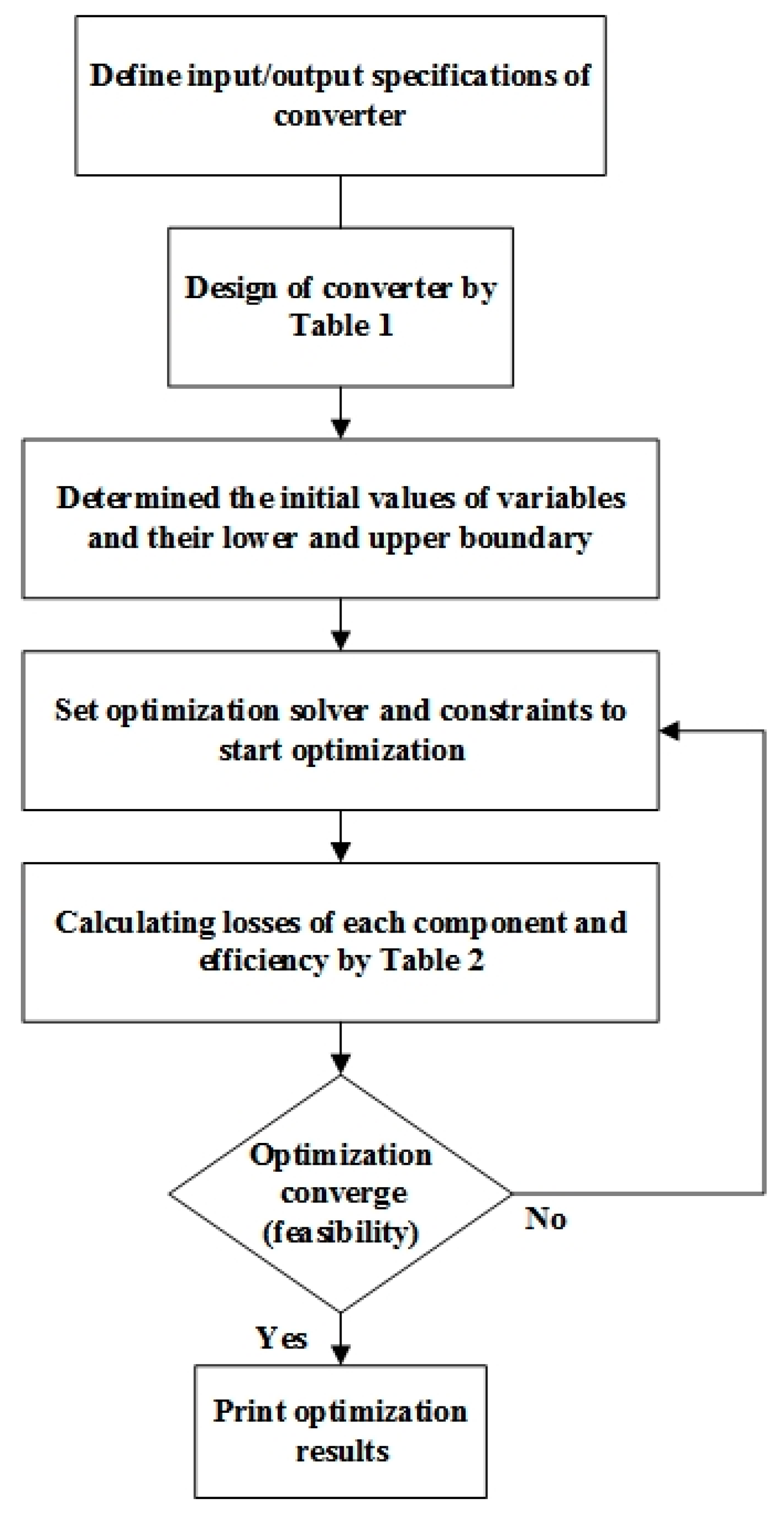
The optimization procedure is shown in Figure 4. Based on the input/output specifications, the start points are calculated by the step-by-step design procedure in Table 1. Then, variables with lower and upper boundaries are determined. After applying the constraints to the solver, the optimization procedure starts. Therefore, efficiency can be calculated easily by knowing the output power of the converter and power losses by [(output power)/(output power + power losses)].

Table 3 shows the load conditions and constraints of variables and the switching frequency range for four different operation modes. In addition,

Table 4. List of components.

Components	Model	Description
MOSFET	IRFP460	$V_{DS}=500V,I_D=20A$
Transformer	EE3314 PC40	Primary: $30\times 0.1\mathrm{mm}$ Secondary: $60\times 0.1\mathrm{mm}$
Resonant inductor	EE28/11 PC40	$30\times 0.1\mathrm{mm}$
Rectifier diode	BYV42E	Dual center tap ultrafast rectifier $V_{RRM}=100\mathrm{V}$ $I_{F(AV)}=2\times 15A$
Resonant Capacitor	$10-45\mathrm{nF},1000\mathrm{V}$	MKP film cap
Output capacitor	$4.7\mathsf{\mu }F$	MKT film cap

shows the list of the components with their manufacturer information to calculate their losses.

Table 5. Losses Profile of LLC resonant converter by Lagrangian optimization method.

Optimum Values: $\mathit{x}=[{\mathit{f}}_{\mathit{s}\mathit{w}}(\mathit{k}\mathit{H}\mathit{z}),{\mathit{L}}_{\mathit{r}}(\mathit{\mu }\mathit{H}),{\mathit{L}}_{\mathit{m}}(\mathit{\mu }\mathit{H}),{\mathit{C}}_{\mathit{r}}(\mathit{n}\mathit{F}),\mathit{n}]$		$[{\mathit{f}}_{\mathit{s}\mathit{w}},{\mathit{L}}_{\mathit{r}},{\mathit{L}}_{\mathit{m}},{\mathit{C}}_{\mathit{r}},\mathit{n}]$ $[80,150,420,22,9]$	$[{\mathit{f}}_{\mathit{s}\mathit{w}},{\mathit{L}}_{\mathit{r}},{\mathit{L}}_{\mathit{m}},{\mathit{C}}_{\mathit{r}},\mathit{n}]$ $[90,140,380,18,2.2]$	$[{\mathit{f}}_{\mathit{s}\mathit{w}},{\mathit{L}}_{\mathit{r}},{\mathit{L}}_{\mathit{m}},{\mathit{C}}_{\mathit{r}},\mathit{n}]$ $[115,130,330,15,7.5]$	$[{\mathit{f}}_{\mathit{s}\mathit{w}},{\mathit{L}}_{\mathit{r}},{\mathit{L}}_{\mathit{m}},{\mathit{C}}_{\mathit{r}},\mathit{n}]$ $[145,95,480,15,4]$
Mode		DCMB	DCMAB	CCMA	DCMA
Components	Power Losses	(W)	(W)	(W)	(W)
Transformer	core	1.186	1.186	1.186	1.186
	copper	0.257	0.202	0.142	0.222
Resonant inductor	core	0.481	0.481	0.481	0.481
	copper	0.212	0.111	0.091	0.119
MOSFETs	Conduction	0.901	0.775	0.325	0.712
	Gate driving	0.019	0.019	0.019	0.019
	Switching	0.081	0.078	0.028	0.029
Rectifier diodes	Conductive loss of VF	2.603	1.967	1.568	1.771
	Conductive loss of rF	0.974	0.804	0.394	0.741
Capacitors	Resonant capacitor	0.161	0.098	0.078	0.092
	Output capacitor	0.188	0.181	0.171	0.177
Total losses		7.063	5.902	4.483	5.549
Efficiency		95.55%	96.26%	97.07%	96.47%

,

Table 6. Losses Profile of LLC resonant converter by LSQ optimization method.

Optimum Values: $\mathit{x}=[{\mathit{f}}_{\mathit{s}\mathit{w}}(\mathit{k}\mathit{H}\mathit{z}),{\mathit{L}}_{\mathit{r}}(\mathit{\mu }\mathit{H}),{\mathit{L}}_{\mathit{m}}(\mathit{\mu }\mathit{H}),{\mathit{C}}_{\mathit{r}}(\mathit{n}\mathit{F}),\mathit{n}]$		$[{\mathit{f}}_{\mathit{s}\mathit{w}},{\mathit{L}}_{\mathit{r}},{\mathit{L}}_{\mathit{m}},{\mathit{C}}_{\mathit{r}},\mathit{n}]$ $[67,166,470,25,8.5]$	$[{\mathit{f}}_{\mathit{s}\mathit{w}},{\mathit{L}}_{\mathit{r}},{\mathit{L}}_{\mathit{m}},{\mathit{C}}_{\mathit{r}},\mathit{n}]$ $[86,140,380,18,2.5]$	$[{\mathit{f}}_{\mathit{s}\mathit{w}},{\mathit{L}}_{\mathit{r}},{\mathit{L}}_{\mathit{m}},{\mathit{C}}_{\mathit{r}},\mathit{n}]$ $[150,115,380,10,8]$	$[{\mathit{f}}_{\mathit{s}\mathit{w}},{\mathit{L}}_{\mathit{r}},{\mathit{L}}_{\mathit{m}},{\mathit{C}}_{\mathit{r}},\mathit{n}]$ $[140,100,350,19,5.5]$
Mode		DCMB	DCMAB	CCMA	DCMA
Components	Power Losses	(W)	(W)	(W)	(W)
Transformer	core	2.328	1.996	1.222	1.387
	copper	1.692	0.952	0.119	0.228
Resonant inductor	core	1.643	1.911	0.496	0.499
	copper	0.792	0.500	0.091	0.189
MOSFETs	Conduction	1.331	0.909	0.423	0.924
	Gate driving	0.019	0.019	0.019	0.019
	Switching	0.361	0.260	0.081	0.101
Rectifier diodes	Conductive loss of VF	2.192	2.249	1.393	1.598
	Conductive loss of rF	1.674	1.423	0.592	0.795
Capacitors	Resonant capacitor	0.366	0.279	0.192	0.310
	Output capacitor	0.261	0.181	0.110	0.293
Total losses		12.659	10.679	4.738	6.343
Efficiency		92.31%	93.43%	96.97%	95.99%

,

Table 7. Losses Profile of LLC resonant converter by modified LSQ optimization method.

Optimum Values: $\mathit{x}=[{\mathit{f}}_{\mathit{s}\mathit{w}}(\mathit{k}\mathit{H}\mathit{z}),{\mathit{L}}_{\mathit{r}}(\mathit{\mu }\mathit{H}),{\mathit{L}}_{\mathit{m}}(\mathit{\mu }\mathit{H}),{\mathit{C}}_{\mathit{r}}(\mathit{n}\mathit{F}),\mathit{n}]$		$[{\mathit{f}}_{\mathit{s}\mathit{w}},{\mathit{L}}_{\mathit{r}},{\mathit{L}}_{\mathit{m}},{\mathit{C}}_{\mathit{r}},\mathit{n}]$ $[70,177,455,22,9.5]$	$[{\mathit{f}}_{\mathit{s}\mathit{w}},{\mathit{L}}_{\mathit{r}},{\mathit{L}}_{\mathit{m}},{\mathit{C}}_{\mathit{r}},\mathit{n}]$ $[90,155,360,15,2.6]$	$[{\mathit{f}}_{\mathit{s}\mathit{w}},{\mathit{L}}_{\mathit{r}},{\mathit{L}}_{\mathit{m}},{\mathit{C}}_{\mathit{r}},\mathit{n}]$ $[135,110,370,13,8.8]$	$[{\mathit{f}}_{\mathit{s}\mathit{w}},{\mathit{L}}_{\mathit{r}},{\mathit{L}}_{\mathit{m}},{\mathit{C}}_{\mathit{r}},\mathit{n}]$ $[130,120,360,15,5.2]$
Mode		DCMB	DCMAB	CCMA	DCMA
Components	Power Losses	(W)	(W)	(W)	(W)
Transformer	core	2.088	1.994	1.310	1.224
	copper	1.698	0.993	0.121	0.278
Resonant inductor	core	1.697	0.998	0.424	0.437
	copper	1.239	0.797	0.298	0.211
MOSFETs	Conduction	1.179	0.990	0.411	0.632
	Gate driving	0.019	0.019	0.019	0.019
	Switching	0.372	0.299	0.072	0.195
Rectifier diodes	Conductive loss of VF	2.810	2.657	1.287	1.398
	Conductive loss of rF	1.762	1.480	0.614	0.889
Capacitors	Resonant capacitor	0.398	0.298	0.162	0.292
	Output capacitor	0.297	0.254	0.103	0.203
Total losses		13.559	10.779	4.821	5.778
Efficiency		91.76%	93.37%	96.92%	96.33%

and

Table 8. Losses Profile of LLC resonant converter by Monte Carlo optimization method.

Optimum Values: $\mathit{x}=[{\mathit{f}}_{\mathit{s}\mathit{w}}(\mathit{k}\mathit{H}\mathit{z}),{\mathit{L}}_{\mathit{r}}(\mathit{\mu }\mathit{H}),{\mathit{L}}_{\mathit{m}}(\mathit{\mu }\mathit{H}),{\mathit{C}}_{\mathit{r}}(\mathit{n}\mathit{F}),\mathit{n}]$		$[{\mathit{f}}_{\mathit{s}\mathit{w}},{\mathit{L}}_{\mathit{r}},{\mathit{L}}_{\mathit{m}},{\mathit{C}}_{\mathit{r}},\mathit{n}]$ $[75,155,420,22,9]$	$[{\mathit{f}}_{\mathit{s}\mathit{w}},{\mathit{L}}_{\mathit{r}},{\mathit{L}}_{\mathit{m}},{\mathit{C}}_{\mathit{r}},\mathit{n}]$ $[85,145,380,18,2.8]$	$[{\mathit{f}}_{\mathit{s}\mathit{w}},{\mathit{L}}_{\mathit{r}},{\mathit{L}}_{\mathit{m}},{\mathit{C}}_{\mathit{r}},\mathit{n}]$ $[120,130,330,15,8.5]$	$[{\mathit{f}}_{\mathit{s}\mathit{w}},{\mathit{L}}_{\mathit{r}},{\mathit{L}}_{\mathit{m}},{\mathit{C}}_{\mathit{r}},\mathit{n}]$ $[135,85,390,18,4]$
Mode		DCMB	DCMAB	CCMA	DCMA
Components	Power Losses	(W)	(W)	(W)	(W)
Transformer	core	1.691	1.212	1.090	1.328
	copper	0.397	0.183	0.122	0.298
Resonant inductor	core	0.599	0.410	0.599	0.582
	copper	0.329	0.143	0.102	0.169
MOSFETs	Conduction	0.892	0.693	0.391	0.690
	Gate driving	0.019	0.019	0.019	0.019
	Switching	0.096	0.067	0.027	0.030
Rectifier diodes	Conductive loss of ${\mathrm{V}}_{\mathrm{F}}$	2.174	1.779	1.633	1.907
	Conductive loss of ${\mathrm{r}}_{\mathrm{F}}$	0.899	0.785	0.654	1.008
Capacitors	Resonant capacitor	0.178	0.100	0.085	0.109
	Output capacitor	0.208	0.191	0.191	0.218
Total losses		7.482	5.582	4.913	6.358
Efficiency		95.30%	96.45%	96.86%	95.98%

show the power loss of each component, and the efficiency is calculated regarding optimum values of variables obtained by the different optimization procedures.

The efficiency is calculated by the following:

$$\eta =\frac{P_{out}}{P_{out}+P_{loss}},$$

(11)

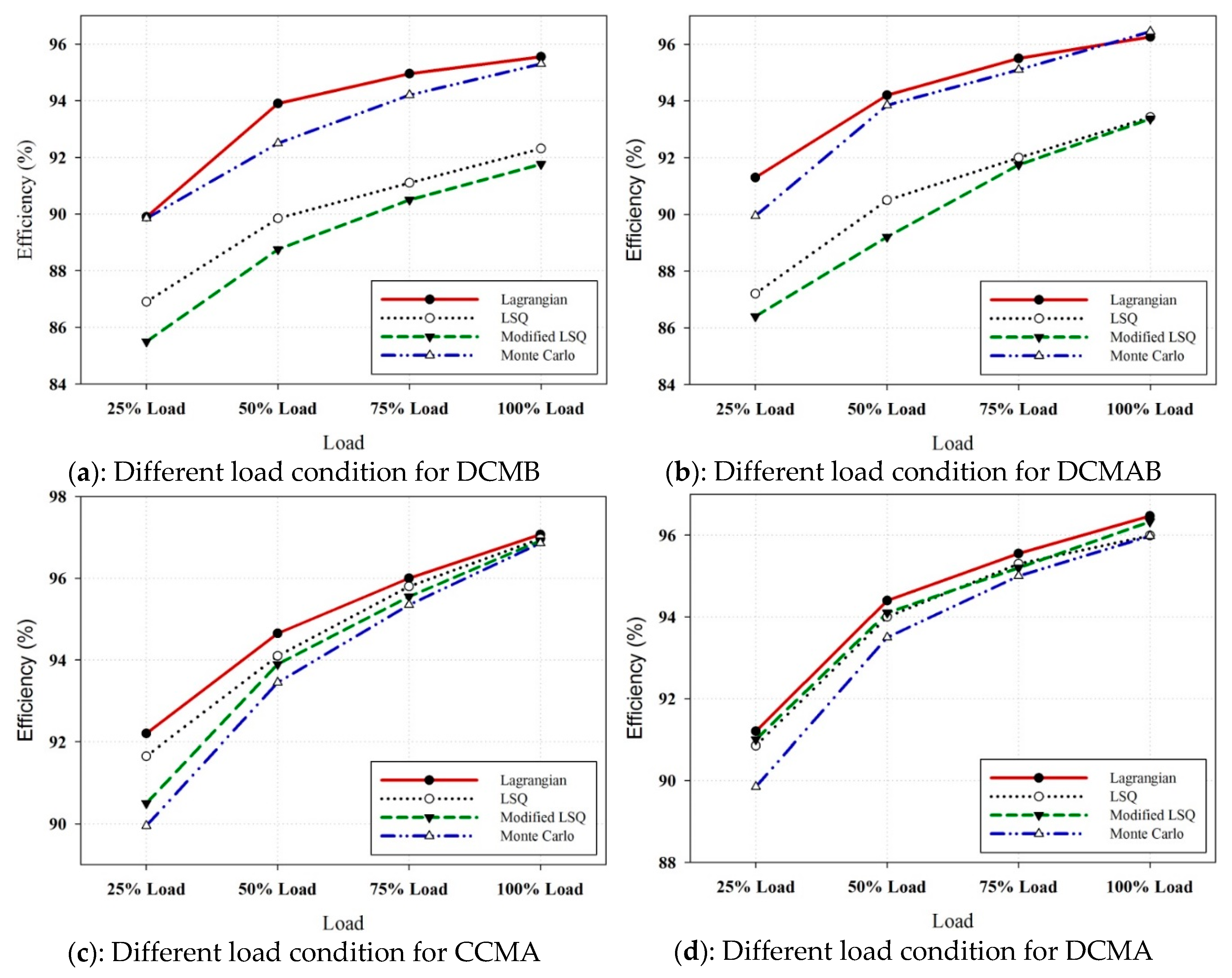
As can be observed from simulation calculations in Table 5, Table 6, Table 7 and Table 8, optimization by the Lagrangian method led to more possible efficiency in all different operation modes. However, this method is very time-consuming due to do many mathematical calculations in comparison with other optimizers. Moreover, the results of the LSQ and modified LSQ are quite similar, though for switching frequencies below the resonant frequency the LSQ optimizer is slightly more efficient than modified LSQ. On the other hand, by comparing the optimum results of Monte Carlo and LSQ, it can be seen that for the operating frequency below resonant frequency the optimum values of variables result in obtaining more efficiency by Monte Carlo optimization procedure, although for upper frequencies, from resonant frequency, the results of LSQ are more valuable.

To compare the efficiencies for different load ranges, Figure 5, Figure 6, Figure 7 and Figure 8 are provided for each operation mode based on the optimum values which are calculated by different optimizers. The figures show that although efficiency decreased by reducing the load, the LLC resonant converter is suitable for high-efficiency power supply in a wide load range.

7. Experimental Results

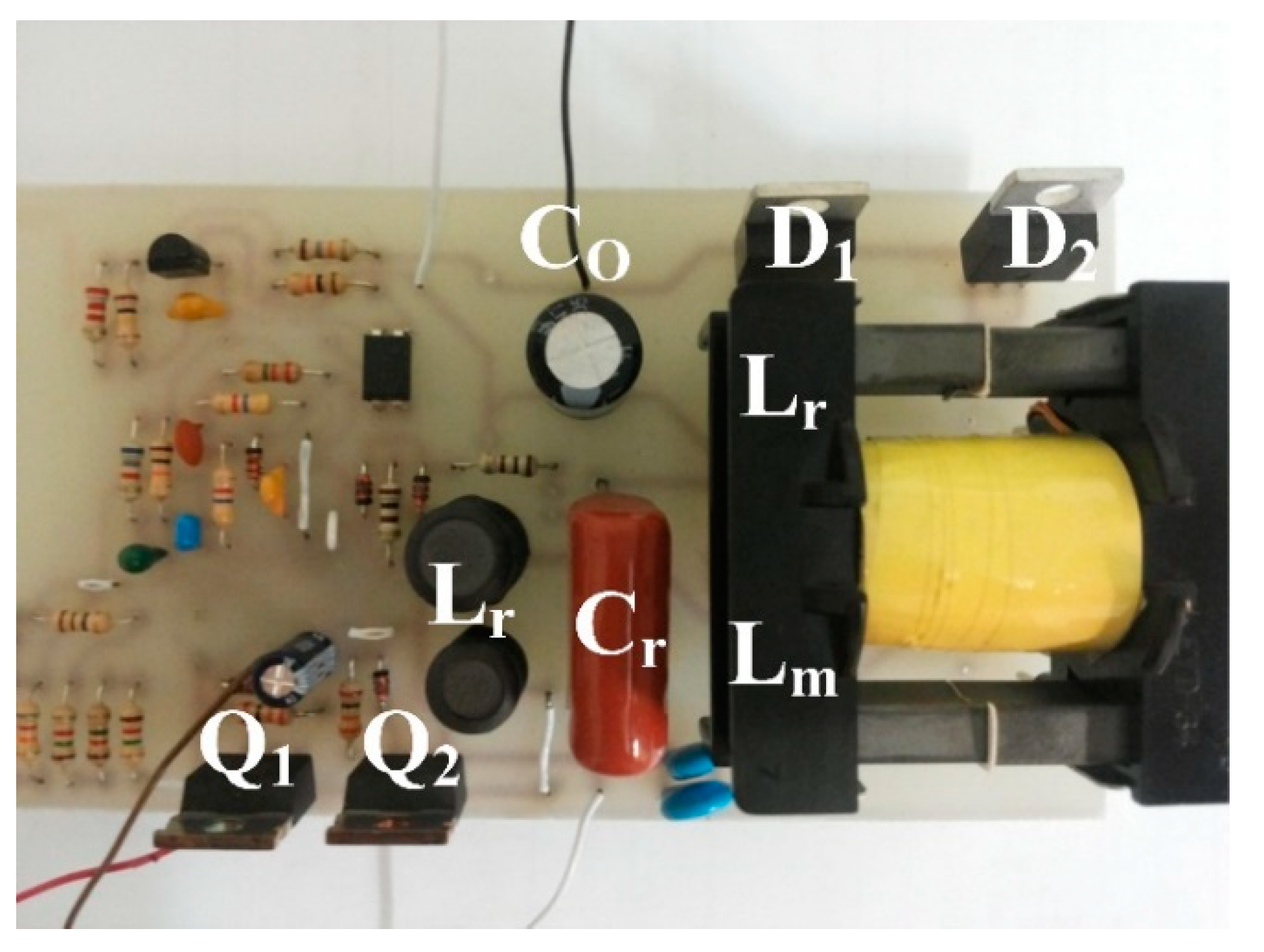
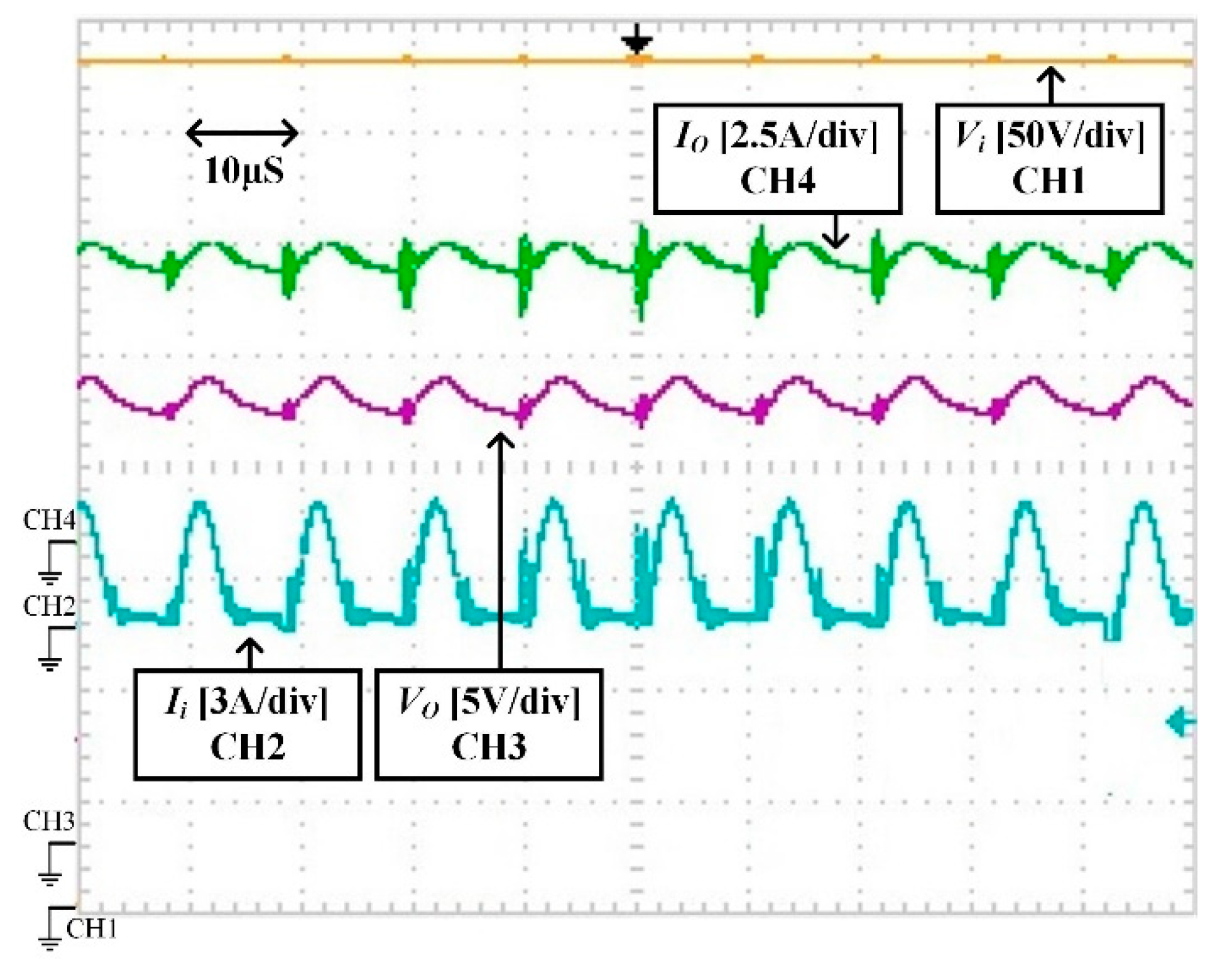
A laboratory prototype of the LLC resonant converter is implemented to calculate the efficiency in different operation modes by the optimum values which are obtained by applying different optimizers. Figure 6 shows the implemented prototype and Figure 7 demonstrates the input and output voltage and current for CCMA operation mode. The efficiency for each operation mode is calculated by [average (output voltage × output current)] / [input voltage × average (input current)].

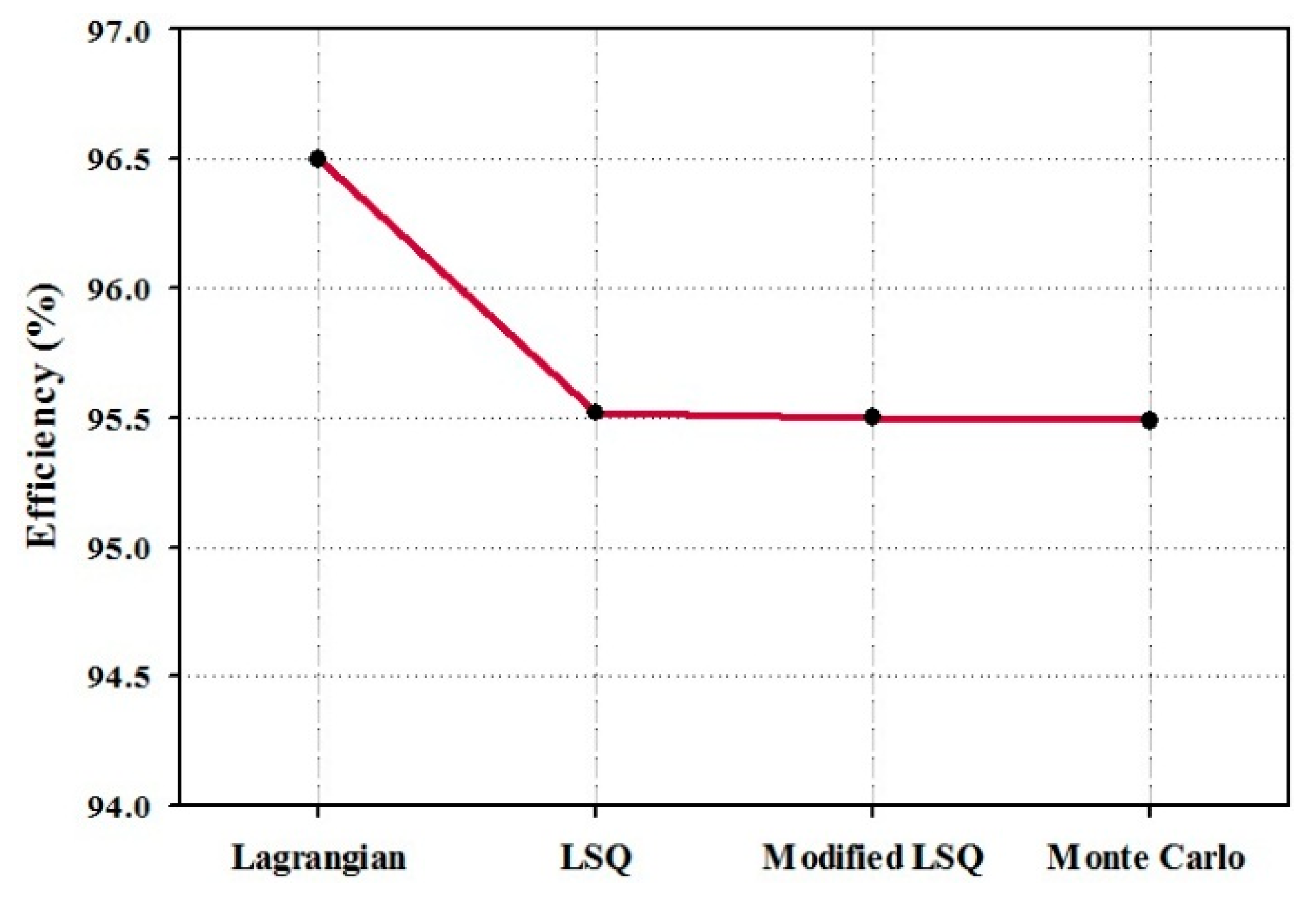
Figure 8 demonstrates the maximum measured efficiency which is possible based on the optimization results; therefore, for all optimization procedures the converter is designed for CCMA. The slight difference between practical result and simulation result refers to unconsidered power loss in the simulation such as printed circuit board (PCB) loss.

8. Conclusions

This paper presents different optimization methods to obtain a highly efficient LLC resonant half-bridge converter. Due to the operating frequency of converter and load condition, the LLC resonant converter can operate in different modes. In this paper, four common optimization methods are applied to the LLC resonant converter in different modes to determine the optimum values for resonant tank components and switching frequency. The results verified that the Lagrangian method is appropriate for all operation modes in LLC resonant converters, although more complicated mathematical calculation is required. However, the results for LSQ and modified LSQ are validated for operating frequency higher than resonant frequency; for below resonant frequency, Monte Carlo led to a more-efficient converter.

References

- Senthamil, L.S.; Ponvasanth, P.; Rajasekaran, V. Design and implementation of LLC resonant half bridge converter. In Proceedings of the 2012 International Conference on Advances in Engineering, Science and Management (ICAESM), Nagapattinam, India, 30–31 March 2012; pp. 84–87. [Google Scholar]
- Park, H.P.; Choi, H.J.; Jung, J.H. Design and implementation of high switching frequency LLC resonant converter for high power density. In Proceedings of the 2015 9th International Conference on Power Electronics and ECCE Asia (ICPE-ECCE Asia), Seoul, Korea, 1–5 June 2015; pp. 502–507. [Google Scholar]
- Guan, Y.; Wang, Y.; Xu, D.; Wang, W. A half-bridge resonant DC/DC converter with satisfactory soft-switching characteristics. Int. J. Circuit Theory Appl. 2017, 45, 120–132. [Google Scholar] [CrossRef]
- Duerbaum, T. First harmonic approximation including design constraints. In Proceedings of the INTELEC—Telecommunications Energy Conference, San Francisco, CA, USA, 4–8 October 1998; pp. 321–328. [Google Scholar]
- Lee, B.H.; Kim, M.Y.; Kim, C.E.; Park, K.B.; Moon, G.W. Analysis of LLC resonant converter considering effects of parasitic components. In Proceedings of the 31st International Telecommunications Energy Conference (INTELEC), Incheon, Korea, 18–22 October 2009; pp. 1–6. [Google Scholar]
- Steigerwald, R.L. A comparison of half-bridge resonant converter topologies. IEEE Trans. Power Electron. 1988, 3, 174–182. [Google Scholar] [CrossRef]
- Prieto, R.; Garcia, O.; Asensi, R.; Cobos, J.A.; Uceda, J. Optimizing the performance of planar transformers. In Proceedings of the Eleventh Annual Applied Power Electronics Conference and Exposition (APEC’96), San Jose, CA, USA, 3–7 March 1996; Volume 1, pp. 415–421. [Google Scholar]
- Trivedi, M.; Shenai, K. Framework for power package design and optimization. In Proceedings of the IEEE International Workshop on Integrated Power Packaging, IWIPP, Chicago, IL, USA, 17–19 September 1998; pp. 35–38. [Google Scholar]
- Gordon, M.H.; Stewart, M.B.; King, B.; Balda, J.C.; Olejniczak, K.J. Numerical optimization of a heat sink used for electric motor drives. In Proceedings of the Conference Record of the IAS’95 Industry Applications Conference, Thirtieth IAS Annual Meeting, 1995 IEEE, Orlando, FL, USA, 8–12 October 1995; Volume 2, pp. 967–970. [Google Scholar]
- Kragh, H.; Blaabjerg, F.; Pedersen, J.K. An advanced tool for optimised design of power electronic circuits. In Proceedings of the Industry Applications Conference, Thirty-Third IAS Annual Meeting, St. Louis, MO, USA, 12–15 October 1998; Volume 2, pp. 991–998. [Google Scholar]
- Piette, N.; Clavel, E.; Marechal, Y. Optimization of cabling in power electronics structure using inductance criterion. In Proceedings of the Industry Applications Conference, Thirty-Third IAS Annual Meeting, St. Louis, MO, USA, 12–15 October 1998; Volume 2, pp. 925–928. [Google Scholar]
- Yu, R.; Ho, G.K.Y.; Pong, B.M.H.; Ling, B.W.K.; Lam, J. Computer-aided design and optimization of high-efficiency LLC series resonant converter. IEEE Trans. Power Electron. 2012, 27, 3243–3256. [Google Scholar] [CrossRef] [Green Version]
- Fang, X.; Hu, H.; Shen, Z.J.; Batarseh, I. Operation mode analysis and peak gain approximation of the LLC resonant converter. IEEE Trans. Power Electron. 2012, 27, 1985–1995. [Google Scholar] [CrossRef]
- De Simone, S.; Adragna, C.; Spini, C.; Gattavari, G. Design-oriented steady-state analysis of LLC resonant converters based on FHA. In Proceedings of the International Symposium on Power Electronics, Electrical Drives, Automation and Motion, SPEEDAM 2006, Taormina, Italy, 23–26 May 2006; pp. 200–207. [Google Scholar]
- Erickson, R.W.; Maksimovic, D. Fundamentals of Power Electronics; Springer Science & Business Media: Berlin, Germany, 2007. [Google Scholar]
- Bertsekas, D.P. Constrained Optimization and Lagrange Multiplier Methods; Academic Press: Cambridge, MA, USA, 2014. [Google Scholar]
- Tourkhani, F.; Viarouge, P.; Meynard, T.A.; Gagnon, R. Power converter steady-state computation using the projected Lagrangian method. In Proceedings of the 28th Annual IEEE Power Electronics Specialists Conference, PESC’97 Record, Saint Louis, MO, USA, 27 June 1997; Volume 2, pp. 1359–1363. [Google Scholar]
- Zhao, B.; Song, Q.; Liu, W. Efficiency characterization and optimization of isolated bidirectional DC–DC converter based on dual-phase-shift control for DC distribution application. IEEE Trans. Power Electron. 2013, 28, 1711–1727. [Google Scholar] [CrossRef]
- Marquardt, D.W. An algorithm for least-squares estimation of nonlinear parameters. J. Soc. Ind. Appl. Math. 1963, 11, 431–441. [Google Scholar] [CrossRef]
- Nye, W.; Riley, D.C.; Sangiovanni-Vincentelli, A.; Tits, A.L. DELIGHT. SPICE: An optimization-based system for the design of integrated circuits. IEEE Trans. Comput. Aided Des. Integr. Circuits Syst. 1988, 7, 501–519. [Google Scholar] [CrossRef]
- Dickman, B.H.; Gilman, M.J. Monte carlo optimization. J. Optim. Theory Appl. 1989, 60, 149–157. [Google Scholar] [CrossRef]
- Yang, G.; Dubus, P.; Sadarnac, D. Analysis of the load sharing characteristics of the series-parallel connected interleaved LLC resonant converter. In Proceedings of the 2012 13th International Conference on Optimization of Electrical and Electronic Equipment (OPTIM), Brasov, Romania, 24–26 May 2012; pp. 798–805. [Google Scholar]
- Yang, C.H.; Liang, T.J.; Chen, K.H.; Li, J.S.; Lee, J.S. Loss analysis of half-bridge LLC resonant converter. In Proceedings of the 2013 1st International Future Energy Electronics Conference (IFEEC), Tainan, Taiwan, 3–6 November 2013; pp. 155–160. [Google Scholar]
© 2018 by the authors. Licensee MDPI, Basel, Switzerland. This article is an open access article distributed under the terms and conditions of the Creative Commons Attribution (CC BY) license (http://creativecommons.org/licenses/by/4.0/).