Seismic Random Noise Attenuation Method Based on Variational Mode Decomposition and Correlation Coefficients

Abstract

Seismic data is easily affected by random noise during field data acquisition. Therefore, random noise attenuation plays an important role in seismic data processing and interpretation. According to decomposition characteristics of seismic signals by using variational mode decomposition (VMD) and the constraint conditions of correlation coefficients, this paper puts forward a method for random noise attenuation in seismic data, which is called variational mode decomposition correlation coefficients VMDC. Firstly, the original signals were decomposed into intrinsic mode functions (IMFs) with different characteristics by VMD. Then, the correlation coefficients between each IMF and the original signal were calculated. Next, based on the differences among correlation coefficients of effective signals and random noise as well as the original signals, the corresponding treatment was carried out, and the effective signals were reconstructed. Finally, the random noise attenuation was realized. After adding random noise to simple sine signals and the synthetic seismic record, the improved complementary ensemble empirical mode decomposition (ICEEMD) and VMDC were used for testing. The testing results indicate that the proposed VMDC has better random noise attenuation effects. It was also used in real-world seismic data noise attenuation. The results also show that it could effectively improve the signal-to-noise ratio (SNR) of seismic data and could provide high-quality basic data for further interpretation of seismic data.

1. Introduction

The seismic signal is a typical nonlinear and nonstationary signal. The seismic exploration process is affected by various factors. There are effective waves and large amounts of random noise in seismic data. Therefore, effective treatment for random noise attenuation could not only improve the signal-to-noise ratio (SNR) and quality of seismic data, but also provide benefit for further interpretation of seismic data, lithology parameter inversion and seismic attributes analyses [1]. At present, there are the median filter method, f-x prediction filter method, polynomial fitting method, wavelet transform and empirical mode decomposition (EMD) method for random noise attenuation in seismic exploration. They have their own advantages and disadvantages. The median filter is a smoothing-based method. By this method, the basic frequency-domain signals tend to shift to low-frequency signals, and the high-frequency signals may be damaged [2,3]. In case of relatively low SNR in high frequency, the f-x prediction filter method may easily cause severe distortion of high-frequency signals and reduce the fidelity of signals and SNR of the seismic profile [4]. The polynomial fitting method requires the original seismic signals to have good continuity. The false seismic events may occur after data processing [5]. In the application of a wavelet transform, the selection of generating functions and de-noising thresholds has significant impacts on the effects of random noise attenuation [6]. EMD has the problems of end effect and mode mixing, which may lead to unsatisfactory effects of random noise attenuation [7].

Variational mode decomposition (VMD) is an adaptive signal processing method put forward by Dragomiretskiy. Compared with EMD, it has stronger noise-resistance ability. Moreover, it could successfully separate two harmonics with very similar frequencies, and the separating effects are not affected by the sampling frequency [8,9,10,11]. Li et al. introduced the principles of VMD and proposed a lateral consistency preserved VMD method [12]. Liu et al. studied the seismic time-frequency representation based on VMD [13]. Li et al. proposed a hybrid de-noising method based on thresholding variational mode decomposition [14]. Li et al. used VMD to analyze the depositional sequence characterization [15]. Jia et al. proposed a method to improve the resolution by using generalized S-transform based on VMD [16]. Zhao et al. extracted intrinsic mode functions (IMFs) based on VMD from seismic amplitudes to constrain self-organizing map facies analysis [17]. Lyu et al. analyzed the discontinuities with VMD-based coherence [18].

Combining VMD with correlation coefficients, this paper developed a new method for seismic data random noise attenuation. VMD was firstly used to decompose the original signals into IMFs with different characteristics. Then, the correlation coefficients between each IMF component and the original signal were calculated. The corresponding treatment was carried out based on differences among correlation coefficients of effective signals, random noise and original signals. The effective signals were reconstructed. Finally, the random noise attenuation was achieved. The results show that the VMDC method performs well in seismic random noise attenuation.

2. Methods

2.1. The Improved Complementary Ensemble Empirical Mode Decomposition ICEEMD

EMD was developed by Huang et al., and is a powerful analytical tool for nonlinear nonstationary signals [19]. However, it has the problems of end effect and mode mixing. ICEEMD was put forward by Tary et al., and this method can solve the above problems to some extent [20,21,22,23]. The calculation steps of this method are as follows:

(1)

Use EMD to calculate the local mean of the i-th iteration $x^i=x+{\epsilon }_0{w}^i$, to get the first residual error.

$$r_1=(1/I){\displaystyle \sum _{i=1}^{I}M[x+{\epsilon }_0{E}_1(w^i)]}$$

(1)

(2)

Calculate the first IMF.

$$IM{F}_1=x-r_1$$

(2)

(3)

Calculate the second residuals and the second IMF.

$$r_2=(1/I){\displaystyle \sum _{i=1}^{I}M(r_1+{\epsilon }_1{E}_2(w^i))}$$

(3)

$$IM{F}_2=r_1-r_2$$

(4)

(4)

When $k=3,\dots ,K$, Calculate the k-th residual error.

$$r_k=(1/I){\displaystyle \sum _{i=1}^{I}M(r_{k-1}+{\epsilon }_{k-1}{E}_k(w^i))}$$

(5)

(5)

Calculate the k-th IMF.

$$IM{F}_k=r_{k-1}-r_k$$

(6)

In the above formula, $E_k(•)$ represents the operator generating the k-th IMF, $M(•)$ represents the operator generating local mean of signal, x is the input signal, $w^i$ is the decomposition of white noise with zero mean unit variance, ${\epsilon }_k$ is a constant greater than zero, $r_i$ is the i-th residuals and I is the number of iterations.

2.2. VMD

In order to avoid the frequency mixture issue of the EMD [19], Dragomiretskiy et al. proposed a signal decomposition method with varying scales, which is the VMD method [8]. Compared with EMD, it has a solid mathematical basis and could be used to effectively solve the mode mixing problem. By VMD, the original signals could be decomposed into k band-limited signals $u_k$ with the center frequency of ${\omega }_k$, where $k$ is the default decomposition scale. It is assumed that each mode function $u_k$ is a limited bandwidth near its center frequency. The adaptive decomposition of the signal is realized by searching the optimal solution of the constrained variational model. The center frequency and bandwidth of each IMF are constantly updated in the iterative solution of the variational model. According to frequency-domain characteristics of actual signals, the adaptive decomposition of the signal band could be completed and some narrow-band IMFs could be obtained.

The steps of estimating the bandwidth of $u_k$ are in the following [8]:

(1) To calculate the analytic function of each $u_k$ and obtain the corresponding one-sided frequency spectrum by Hilbert transform.

(2) To adjust the estimated central spectrum by adding exponential terms and modulate the frequency spectrum of each mode into the corresponding basic frequency band.

(3) To estimate the bandwidth by Gaussian smoothness of the demodulated signal and gradient energy criterion.

By following the aforementioned steps, the obtained constrained variational problem is as follows:

$$\begin{array}{c}\underset{\left\{{\mu }_k\right\},\left\{{\omega }_k\right\}}{\min }\left\{{\displaystyle \sum _k{\Vert {\partial }_t\left[(\delta (t)+\frac{j}{\pi t})*u_k(t)\right]\exp (-j{\omega }_{k}t)\Vert }_2^2}\right\},\\ s.t.\begin{array}{cc}& {\displaystyle \sum _k{u}_k}=x(t)\end{array},\end{array}$$

(7)

where $\left\{u_k\right\}=\left\{u_1,u_2,\dots ,u_k\right\}$ is the function of each mode. $\left\{{\omega }_k\right\}=\left\{{\omega }_1,{\omega }_2,\dots ,{\omega }_k\right\}$ is the center frequency and ${\displaystyle \sum _k=}{\displaystyle \sum _{k=1}^K}$ is the sum of each mode.

(4) To transform the above constrained variational problem into an unconstrained variational problem by introducing the Lagrange multiplier $\lambda (t)$ and two-penalty factor, the formula of the augmented Lagrange multiplier could be obtained, as follows:

$$\begin{array}{l}L(\left\{u_k\right\},\left\{{\omega }_k\right\},\lambda )=\\ \alpha {{\displaystyle \sum _k\Vert {\partial }_t\left[(\delta (t)+\frac{j}{\pi t})u_k(t)\right]\exp (-j{\omega }_{k}t)\Vert }}_2^2+\\ {\Vert x(t)-{\displaystyle \sum _k{u}_k(t)}\Vert }_2^2+\langle \lambda (t),x(t)-{\displaystyle \sum _k{u}_k(t)}\rangle \end{array}.$$

(8)

The alternating direction method of multipliers is applied to solve the above variational problems. The iterative optimization of $u^{k+1}$, ${\omega }_k^{k+1}$ and ${\lambda }^{k+1}$ could get the saddle points of the augmented Lagrange multiplier. The iteration steps are as follows:

(1) To initialize $u^1$, ${\omega }_{}^1$, ${\lambda }^1$, $n=0$.

(2) If $n=n+1$, to perform the whole loop.

(3) To execute the first inner loop, update $u_k$ according to ${\omega }_k^{k+1}=\arg \underset{u^k}{\min }L(\left\{u_{i<k}^{n+1}\right\},\left\{u_{i\ge k}^n\right\},\left\{{\omega }_i^n\right\},{\lambda }^n)$.

(4) $k=k+1$, and repeat step (3) until the completion of the first loop when $k=K$.

(5) To execute the second inner loop and update $\lambda$ according to ${\lambda }^{n+1}={\lambda }^n+\tau (x(t)-{\displaystyle \sum _k{u}_{{}_k}^{n+1}})$.

(6) To repeat step 2 and step 5 until meeting ${\displaystyle \sum _k({\Vert u_k^{n+1}-u_k^n\Vert }_2^2/{\Vert u_k^n\Vert }_2^2)}<\epsilon$. The whole looping will end and $k$ IMFs could be obtained.

2.3. Correlation Coefficient Method

The Pearson correlation coefficient (PCC) is a statistical method to quantitatively measure correlations between two random variables. One of its important mathematical characteristics is that the variations of positions and scales will not cause the changes of correlation coefficients, so it is suitable for correlation evaluation of geophysical data [24,25,26]. The Pearson correlation coefficient could be expressed as follows [27]:

$$\begin{array}{l}\rho =\frac{\mathrm{cov}(X,Y)}{{\sigma }_X{\sigma }_Y}=\frac{E(XY)-E(X)E(Y)}{\sqrt{E(X^2)-E^2(X)}\sqrt{E(Y^2)-E^2(Y)}}\\ =\frac{{\displaystyle \sum (x_i-\overline{x})(y_i-\overline{y})}}{\sqrt{{\displaystyle \sum {(x_i-\overline{x})}^2}}\sqrt{{\displaystyle \sum {(y_i-\overline{y})}^2}}}\end{array}$$

(9)

where $\mathrm{cov}(X,Y)$ refers to covariance of $X$ and $Y$. ${\sigma }_X$ and ${\sigma }_Y$ are the standard deviations. $\overline{x}=E(X)$ and $\overline{y}=E(Y)$ are the expected values of $X$ and $Y$, respectively. The bigger the absolute values of the correlation coefficients, the stronger the correlation. The closer the correlation coefficient is to 1 or −1, the stronger the correlation between $X$ and $Y$. The closer the correlation coefficient is to 0, the weaker the correlation between $X$ and $Y$. Generally, the correlation intensity among variables could be judged according to

Table 1. Person correlation coefficients and correlation intensity.

Absolute Value of Pearson Correlation Coefficient (PCC)	Correlation Intensity
0.8–1.0	Extremely strong correlation
0.6–0.8	Strong correlation
0.4–0.6	Medium correlation
0.2–0.4	Weak correlation
0.0–0.2	Extremely weak correlation or no correlation

, as follows:

Table 1 shows that when the correlation coefficient is greater than 0.4, $X$ and $Y$ have good correlation. If the correlation coefficient is less than 0.2, the correlation coefficient of $X$ and $Y$ is poor. When the correlation coefficient is 0.2–0.4, the correlation between $X$ and $Y$ is general.

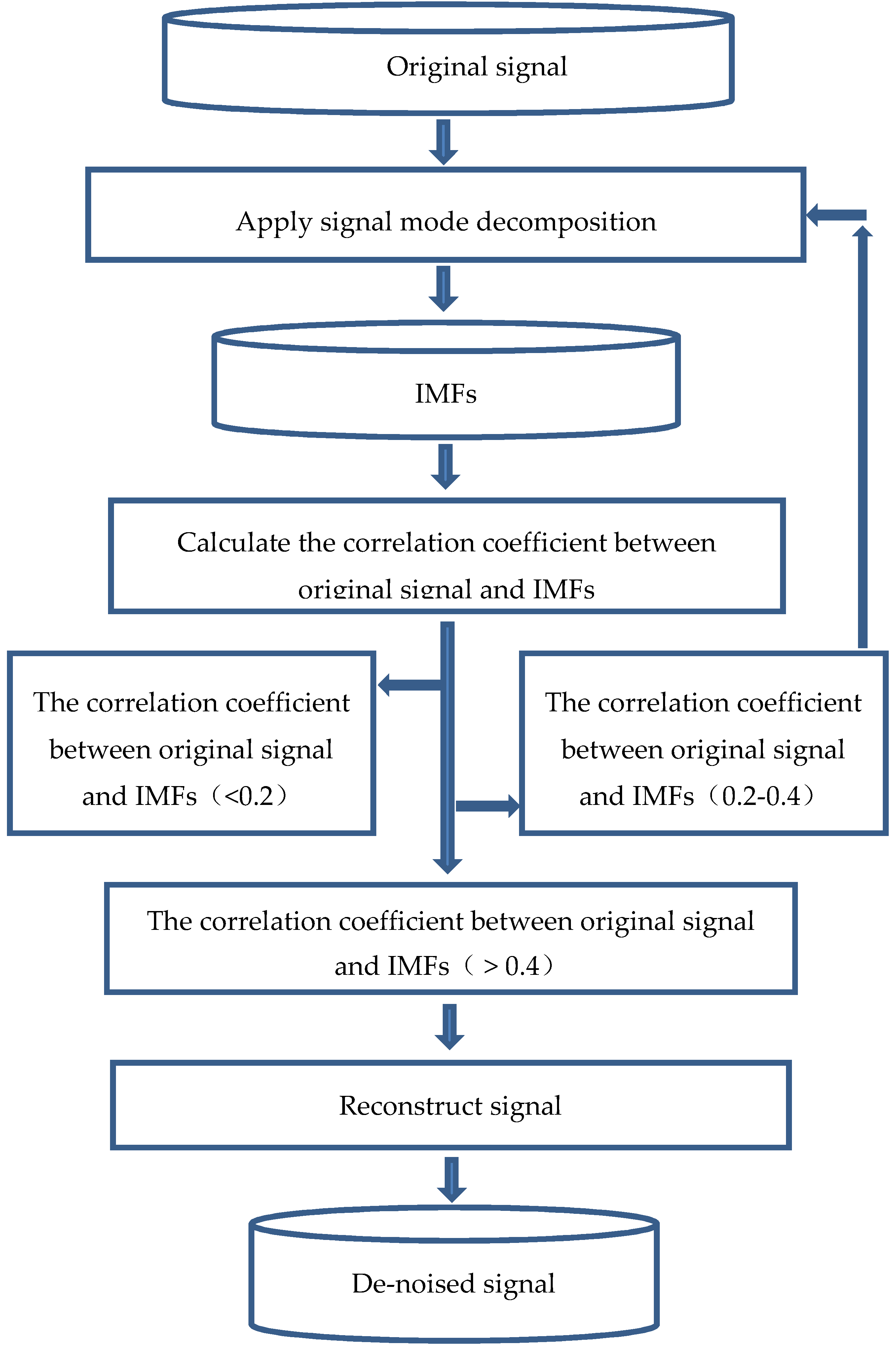
2.4. Random Noise Attenuation Method Based on VMD and Correlation Coefficients

It was assumed that a random noise signal was made of a noise-free signal and random noise. The VMD algorithm was firstly used to decompose the target signals into various IMFs which may include effective signals, effective signals with partial noise, and noise signals. Formula (9) was used to calculate the correlation coefficients between each IMF and the original signal. Then, on this basis, the effective signals were reconstructed. The reconstruction principles are as follows:

(1) The correlation coefficient of less than 0.2 represented that the IMF component had no correlation with the original signal, and had only the random noise, so the IMF component did not participate in signal reconstruction.

(2) The correlation coefficient of bigger than 0.4 represented that there was good correlation between the IMF component and the original signal, so the IMF component participated in signal reconstruction.

(3) The correlation coefficient between 0.2 and 0.4 represented that there was weak correlation between the IMF component and the original signal. The IMF component contained the effective signal and random noise. It was decomposed into $s_n=s_k+n_k$, where $s_k$ denotes the effective signal and $n_k$ denotes the residual random noise. Then, the VMD was used for IMF treatment to get $s_k$ and $n_k$. $s_k$ participated in the signal reconstruction. The process of random noise attenuation based on VMDC is shown in Figure 1.

3. Theoretical Model Test

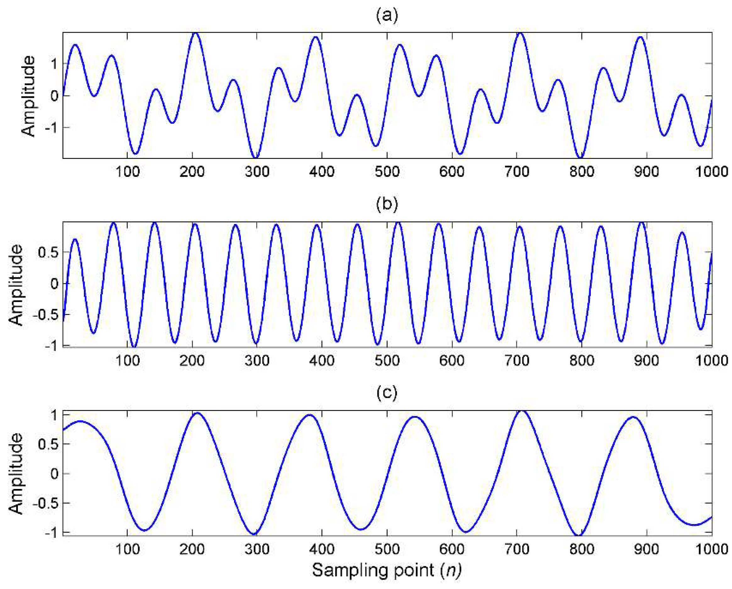
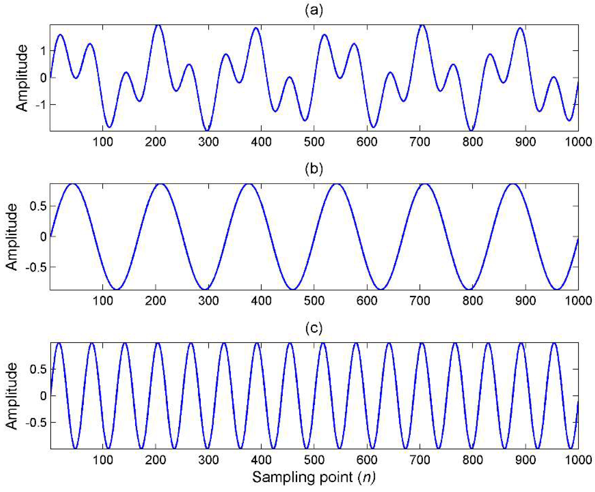
3.1. Simple Signal Model Test

The simple signal was expressed as $z(t)=x1(t)+x2(t)$, where $x1(t)=\sin (12\times \pi \times t)$ and $x2(t)=\sin (32\times \pi \times t)$. The number of sampling points was 1000. ICEEMD and VMD were used for signal decomposition. The results are shown in Figure 2 and Figure 3. Developed by Colominas et al., ICEEMD has developed the EMD and could solve the problems of modal mixing in the application of EMD [20,28]. As shown in Figure 2 and Figure 3, ICCEMD decomposes signals according to the frequency from high to low, while the VMD was the opposite. When the signal did not contain noise, the correlation coefficients between the decomposed signals by ICEEMD and VMD and the original signals could reach more than 0.97. In terms of calculation efficiency, ICEEMD took 21.96 s while VMD took only 2.15 s.

The above results show that both ICEEMD and VMD have good decomposition effects, and VMD has higher calculation efficiency.

20% random noise was added to the above simple signal using z(t) = x1(t)+x2(t)+0.2*rand(t). Figure 4 and Figure 5 show the decomposition results by ICEEMD and VMD, respectively. In Figure 4, some IMF components contained modal mixing, which affected the reconstructed signals after superposition of the IMFs. By VMD, the correlation coefficients between each IMF and the original signal were calculated to be 0.73, 0.70 and 0.03. According to the principles of signal reconstruction in Section 2.3, IMF3 did not participate in signal reconstruction. Figure 6 shows the reconstruction results of IMF1 and IMF2. The blue line denotes the signals without noise, and the red line denotes the reconstruction results. The correlation coefficient between the decomposition signal and the original signal was 0.99 and the root mean square error (RMSE) was only 0.0985. In terms of calculation efficiency, ICEEMD took 22.90 s while VMD only took 0.51 s.

The above results indicate that VMD still has good decomposition effects with random noise in signals. Moreover, it is more beneficial to suppress random noise with higher operating efficiency.

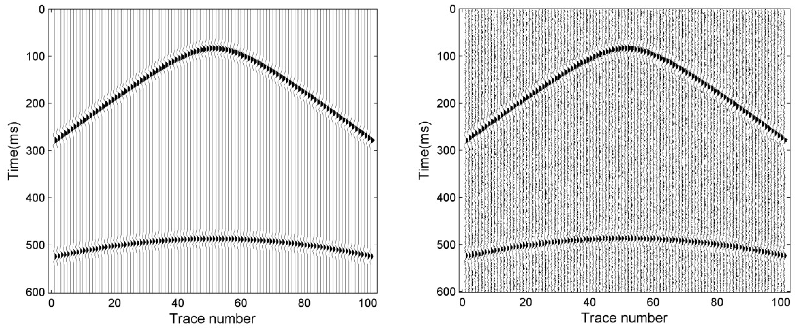
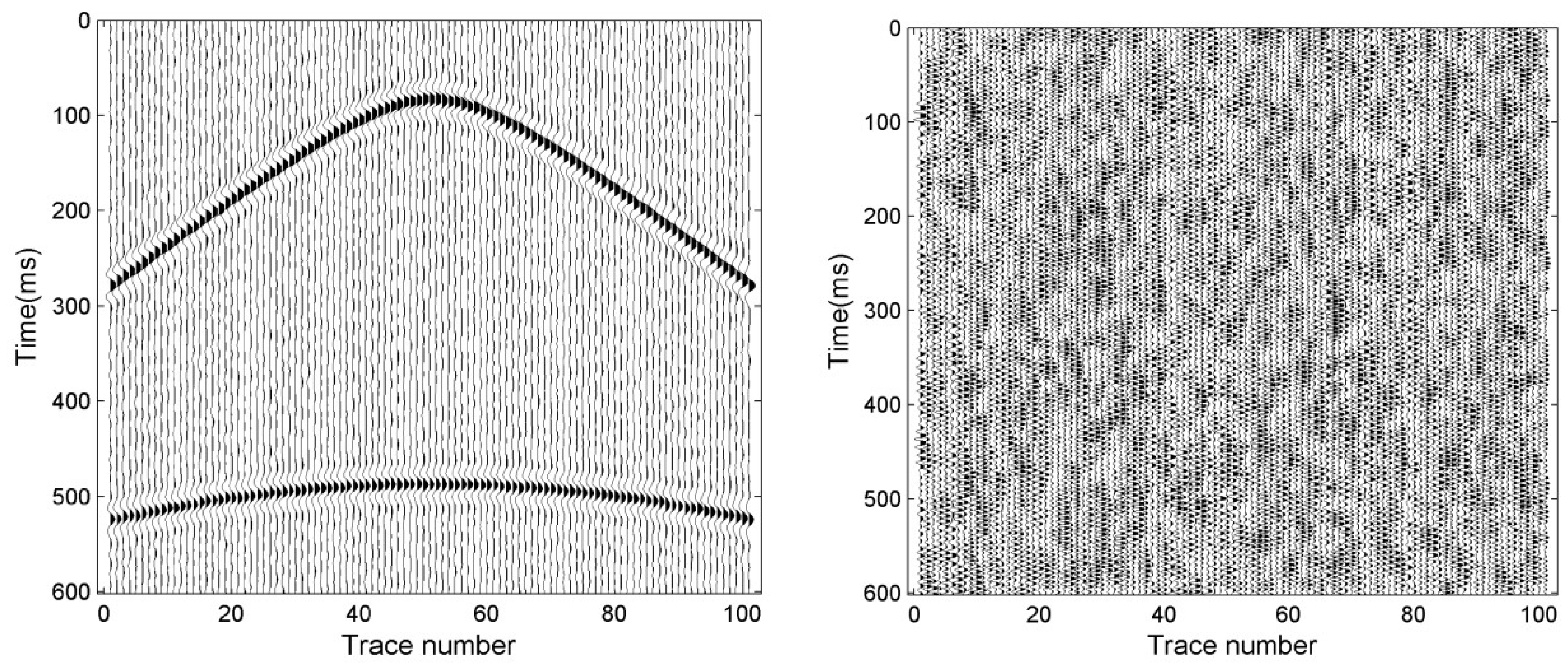
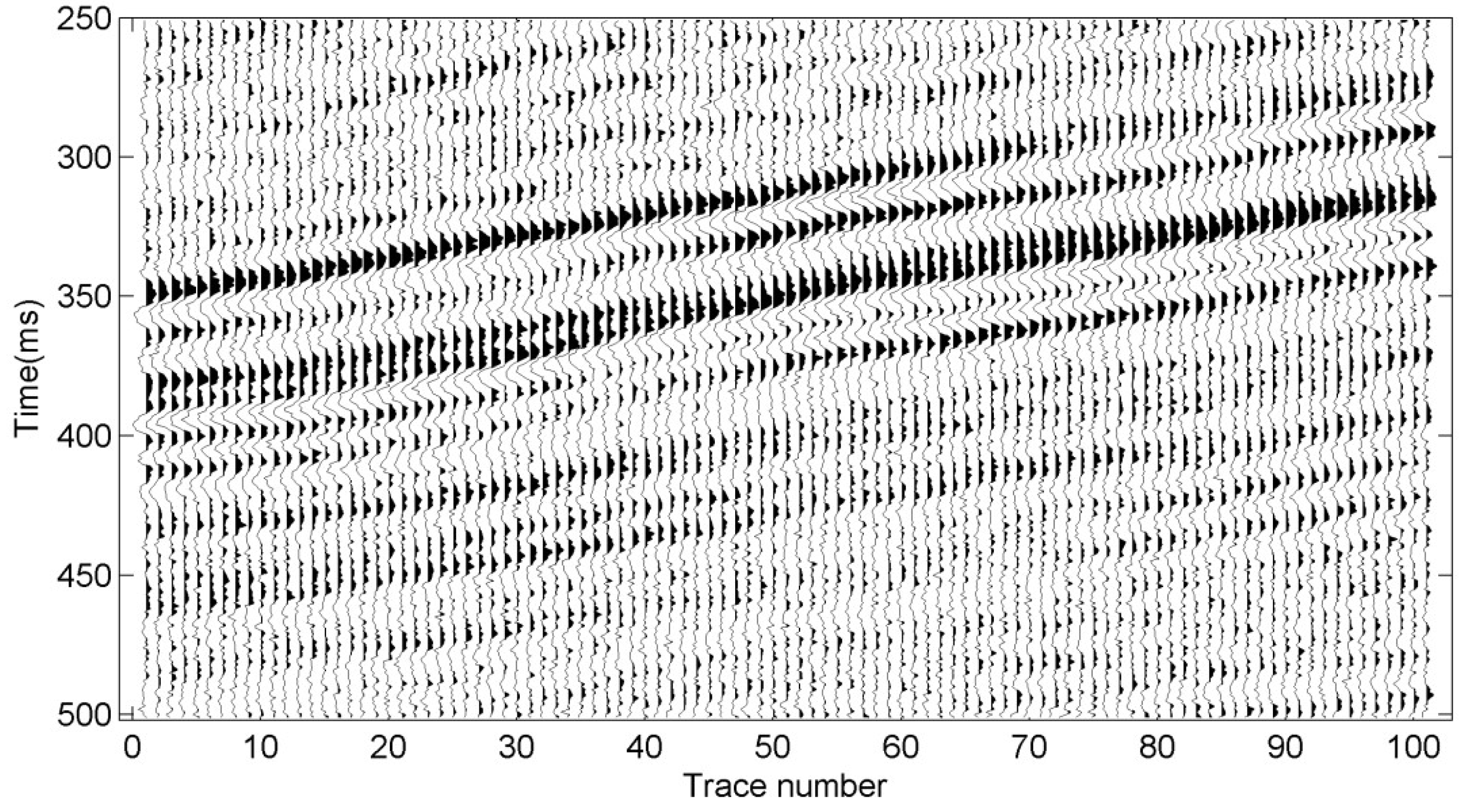
3.2. Synthetic Seismic Records Model Test

To further test the new method’s application effects in seismic data processing, the synthetic seismic records model test was conducted after adding random noise. This paper established synthetic seismic records with the sampling interval of 0.1 ms and the dominant frequency of the wavelet of 45 HZ, and the synthetic seismic records with 20% random noise, as shown in Figure 7. The comparison in Figure 7 shows that after adding noise, the SNR of the synthetic seismic records was reduced, the events became blurred and some information of seismic horizons was masked by the random noise.

The decomposition of synthetic seismic records with 20% random noise by ICEEMD could obtain the seismic records and noise profiles, as shown in Figure 8. It could be seen that there was strong random noise in the profile after suppressing the random noise. Figure 9 shows the seismic records after suppressing the random noise by the VMDC. Compared with the noise attenuation results by ICEEMD and VMDC, the de-noising effects by the VMDC are superior to the effects by ICEEMD. In Figure 9, the seismic events were better restored and the SNR was greatly improved. In addition, the noise in Figure 8 contained a small amount of effective waves, while noise was dominant in Figure 9.

The above results show that, under the synthetic seismic records with the random noise, the reconstructed events by the VMDC are more obvious and continuous, and the random noise reduction effects are better.

4. Case Study

To fully verify the application effects of the proposed VMDC in real-world seismic data, this paper selected the 3-D seismic data in Inner Mongolia in China to carry out the test. The acquisition of seismic data was in the winter, so the wind was blowing very hard. At the same time, the gangue field and air shafts were under construction. What is worse, the random noise interference was more serious in this area because there were many vehicles in adjacent industrial areas. Figure 10 shows the actual seismic profiles with random noise. It could be found that the existing random noise reduced the SNR of the seismic data and influenced the continuity of events in seismic records.

The ICEEMD and the VMDC were used for noise attenuation of post-stack seismic data. The signal reconstruction process was introduced by taking the 50th channel as an example. Firstly, ICEEMD and VMDC were used to decompose seismic signals. Then, by ICEEMD, the correlation coefficients between each IMF and the original signal were calculated as 0.1432, 0.5058 and 0.7329. By VMD, the correlation coefficients between each IMF and the original signal were calculated as 0.7221, 0.6611 and 0.1156. Therefore, the IMF2 and IMF3 decomposed by ICEEMD, and IMF1 and IMF2 decomposed by VMDC, participated in the signal constructions. The signals in other seismic traces were reconstructed by similar steps, as shown in Figure 11 and Figure 12. Through the comparative analysis of Figure 10, Figure 11 and Figure 12, it is found that both ICEEMD and the VMDC could suppress the random noise to a certain extent, and the latter could significantly enhance the continuity of events.

Above all, the VMDC method proposed in this paper has obvious noise attenuation effects and could make the events more clear and continuous. What is more, it could improve the SNR of seismic data and the smoothing of each channel of the seismic record. It also could better reflect shapes of strata. It is shown that the method could achieve good effects in random noise attenuation in real-world seismic data.

5. Conclusions

This paper proposed a new method for seismic random noise attenuation based on VMD and correlation coefficients, called VMDC. Under the situation of simple sine signals without noise, both ICEEMD and VMDC have better decomposition results, and VMDC has better calculation efficiency. After adding random noise to the simple sine signals and the synthetic seismogram, the testing results show that the VMDC has better noise attenuation effects. The application results in real-world seismic data indicate that the new method could significantly improve the SNR of seismic data, enhance the continuity of events as well as provide reliable basic data for further seismic data interpretation.

References

1. Yan, Z.H.; Luan, X.W.; Wang, Y.; Pan, J.; Fang, G.; Shi, J. Seismic random noise attenuation based on empirical mode decomposition of fractal dimension. Chin. J. Geophys. 2017, 60, 2845–2857. (In Chinese) [Google Scholar] [CrossRef]
2. Liu, C.; Liu, Y.; Yang, B.J.; Wang, D.; Sun, J.G. A 2D multistage median filter to reduce random seismic noise. Geophysics 2006, 71, V105–V110. [Google Scholar] [CrossRef]
3. Liu, Y.K. Noise reduction by vector median filtering. Geophysics 2013, 78, 79–86. [Google Scholar] [CrossRef]
4. Abbas, K.; Abdolrahim, J. Random noise reduction by F-X deconvolution. J. Earth 2010, 5, 61–68. [Google Scholar]
5. Liu, G.C.; Chen, X.H.; Li, J.Y.; Du, J.; Song, J.W. Seismic noise attenuation using nonstationary polynomial fitting. Appl. Geophys. 2011, 8, 18–26. [Google Scholar] [CrossRef]
6. Zhang, Z.H.; Sun, C.Y.; Tang, J.; Xiao, G.R.; Li, L.J. A denoising method based on combined Curvelet and Wavelet transform. In Proceedings of the Beijing 2014 International Geophysical Conference and Exposition, Beijing, China, 21–24 April 2014. [Google Scholar]
7. Huang, Y.P.; Di, H.B.; Malekian, R.; Qi, X.M.; Li, Z.X. Noncontact measurement and detection of instantaneous seismic attributes based on complementary ensemble empirical mode decomposition. Energies 2017, 10, 1655. [Google Scholar] [CrossRef]
8. Dragomiretskiy, K.; Zosso, D. Variational mode decomposition. IEEE Trans. Signal Process. 2014, 62, 531–544. [Google Scholar] [CrossRef]
9. Glowacz, A.; Glowacz, W.; Glowacz, Z.; Kozik, J. Early fault diagnosis of bearing and stator faults of the single-phase induction motor using acoustic signals. Measurement 2018, 113, 1–9. [Google Scholar] [CrossRef]
10. Glowacz, A. Fault diagnosis of single-phase induction motor based on acoustic signals. Mech. Syst. Signal Process. 2019, 117, 65–80. [Google Scholar] [CrossRef]
11. Li, Z.X.; Jiang, Y.; Guo, Q.; Hu, C.; Peng, Z.X. Multi-dimensional variational mode decomposition for bearing-crack detection in wind turbines with large driving-speed variations. Renew. Energy 2016, 116, 55–73. [Google Scholar] [CrossRef]
12. Li, F.Y.; Zhao, T.; Qi, X.; Marfurt, K.J.; Zhang, B. Lateral consistency preserved Variational Mode Decomposition. In SEG Technical Program Expanded Abstracts 2016; Society of Exploration Geophysicists: Dallas, TX, USA, 21 October 2016. [Google Scholar]
13. Liu, W.; Cao, S.Y.; Chen, Y.K. Applications of variational mode decomposition in seismic time-frequency analysis. Geophysics 2016, 81, V365–V378. [Google Scholar] [CrossRef]
14. Li, F.Y.; Zhang, B.; Verma, S.; Marfurt, K.J. Seismic signal denoising using thresholded variational mode decomposition. Explor. Geophys. 2017, 49, 450–461. [Google Scholar] [CrossRef]
15. Li, F.Y.; Zhang, B.; Zhai, R.; Zhou, H.L.; Marfurt, K.J. Depositional sequence characterization based on seismic variational mode decomposition. Interpretation 2017, 5, SE97–SE106. [Google Scholar] [CrossRef]
16. Jia, J.F.; Chen, X.H.; Jiang, S.H.; Jiang, W.; Zhang, J. Resolution enhancement in the generalized S-transform domain based on variational-mode decomposition of seismic data. In Proceedings of the International Geophysical Conference, Qingdao, China, 17–20 April 2017. [Google Scholar]
17. Zhao, T.; Li, F.Y.; Marfurt, K.J. Constraining self-organizing map facies analysis with stratigraphy: An approach to increase the credibility in automatic seismic facies classification. Interpretation 2017, 5, T163–T171. [Google Scholar] [CrossRef]
18. Lyu, B.; Li, F.Y.; Zhao, T.; Marfurt, K.J. Highlighting discontinuities with variational-mode decomposition-based coherence. In SEG Technical Program Expanded Abstracts 2018; Society of Exploration Geophysicists: Anaheim, CA, USA, 19 October 2018. [Google Scholar]
19. Huang, N.E.; Shen, Z.; Long, S.R.; Wu, M.C.; Shih, H.H.; Zheng, Q.; Liu, H.H. The empirical mode decomposition and the Hilbert spectrum for nonlinear and non-stationary time series analysis. Proc. R. Soc. Lond. A Math. Phys. Eng. Sci. 1998, 454, 903–995. [Google Scholar] [CrossRef]
20. Tary, J.B.; Herrera, R.H.; Han, J.; Baan, M.V.D. Spectral estimation—What is new? what is next? Rev. Geophys. 2014, 52, 723–749. [Google Scholar] [CrossRef]
21. Han, J.; Mirko, V.D.B. Microseismic and seismic denoising via ensemble empirical mode decomposition and adaptive thresholding. Geophysics 2015, 80, KS69–KS80. [Google Scholar] [CrossRef]
22. Wang, Z.G.; Gao, J.H.; Wang, P.; Jiang, X.D. The analytic wavelet transform with generalized Morse wavelets to detect fluvial channels in the Bohai Bay Basin, China. Geophysics 2016, 81, O1–O9. [Google Scholar] [CrossRef]
23. Chen, W.; Song, H. Automatic noise attenuation based on clustering and empirical wavelet transform. J. Appl. Geophys. 2018, 159, 649–665. [Google Scholar] [CrossRef]
24. Chen, Z.A.; Wu, X.Y. Accuracy of measuring velocity improved by correlative analysis method. Prog. Geophys. 2001, 16, 101–103. (In Chinese) [Google Scholar] [CrossRef]
25. Cui, Z.J.; Li, Z.X.; Chen, Z.L. A study on the new method for determining small earthquake sequence type-Correlation analysis of spectral amplitude. Chin. J. Geophys. 2012, 55, 1718–1724. (In Chinese) [Google Scholar] [CrossRef]
26. Yin, C.C.; Sun, S.Y.; Cao, X.H.; Liu, Y.H.; Chen, H. 3D joint inversion of magnetotelluric and gravity data based on local correlation constraints. Chin. J. Geophys. 2018, 61, 358–367. (In Chinese) [Google Scholar] [CrossRef]
27. Rodgers, J.L.; Nicewander, W.A. Thirteen ways to look at the correlation coefficient. Am. Stat. 1988, 42, 59–66. [Google Scholar] [CrossRef]
28. Colominas, M.A.; Schlotthauer, G.; Torres, M.E. Improved complete ensemble emd: A suitable tool for biomedical signal processing. Biomed. Signal Process. Control 2014, 14, 19–29. [Google Scholar] [CrossRef]
Figure 1. Flow chart of VMDC.
Electronics 07 00280 g001
Figure 2. Decomposition of the artificially mixed signal by improved complementary ensemble empirical mode decomposition (ICEEMD): (a) the mixed signal; (b) IMF1 (intrinsic mode function 1) of the signal; (c) IMF2 of the signal.
Electronics 07 00280 g002
Figure 3. Decomposition of the artificially mixed signal by variational mode decomposition (VMD): (a) the mixed signal; (b) IMF1 of the signal; (c) IMF2 of the signal.
Electronics 07 00280 g003
Figure 4. Decomposition of the artificially mixed signal with 20% additive noise by ICEEMD: (a) the signal; (b) IMF1 of the signal; (c) IMF2 of the signal; (d) IMF3 of the signal; (e) IMF4 of the signal; and (f) IMF5 of the signal.
Electronics 07 00280 g004
Figure 5. Decomposition of the artificially mixed signal with 20% additive noise by VMD: (a) the signal; (b) IMF1 of the signal; (c) IMF2 of the signal; (d) IMF3 of the signal.
Electronics 07 00280 g005
Figure 6. Reconstruction results by VMDC (red) and the original signals without noise (blue).
Electronics 07 00280 g006
Figure 7. Synthetic seismic records without noise (left) and with 20% noise (right).
Electronics 07 00280 g007
Figure 8. Random noise attenuation results (left) and the noise (right) by ICEEMD.
Electronics 07 00280 g008
Figure 9. Random noise attenuation results (left) and the noise (right) by VMDC.
Electronics 07 00280 g009
Figure 10. The original seismic data.
Electronics 07 00280 g010
Figure 11. Random noise attenuation results by ICEEMD.
Electronics 07 00280 g011
Figure 12. Random noise attenuation results by VMDC.
Electronics 07 00280 g012