Near Field Antenna Measurement Sampling Strategies: From Linear to Nonlinear Interpolation

Abstract

The aim of this review paper is to discuss some of the advanced sampling techniques proposed in the last decade in the framework of planar near-field measurements, clarifying the theoretical basis of the different techniques, and showing the advantages in terms of number of measurements. Instead of discussing the details of the techniques, the attention is focused on their theoretical bases to give a gentle introduction to the techniques. For each sampling method, examples on a liner array are discussed to clarify the advantages and disadvantages of the method.

1. Introduction

Antenna measurement is an active field of research, with large industrial impact. Effective measurement techniques include Far-Field (FF), compact range, and Near-Field (NF) systems [1]. Among them, NF techniques are becoming the most commonly adopted method in both industries and universities. These facilities allow performing accurate measurements of the NF distribution in a controlled environments and, in the next step, an accurate evaluation of the far field using Near Field-Far Field (NF-FF) transformation [2]. In this process, some signal processing methods can be applied to improve the far-field accuracy, which is discussed in Section 4.

Near field measurements can be affected by many causes of uncertainty, including the finite size of the scanning area where the field radiated by the Antenna Under Test (AUT) is measured, the presence of reflections and scattering from the environment, small shifts of the measurement positions, the use of non-ideal probes, the presence of multiple reflection between the AUT and the probe, and an erroneous sampling of the near-field that does not allows collecting all the information required for the NF-FF transformation process [3].

This paper is focused on the last aspect, i.e., the sampling process of the electromagnetic field radiated by the AUT. Indeed, how many measurements points and where to measure the field in the space are fundamental problems in NF measurements [4,5].

As is well known, in planar NF systems, the relationship between NF and FF is basically a Fourier Transform [6]. Starting from this observation, theorems for data sampling were developed using the Nyquist–Shannon theory of bandlimited functions. The result is the $\lambda /2$ spatial sampling step [1] that is currently universally adopted in planar near-field measurements.

This paper presents some novel sampling strategies developed in the last decades. It must be stressed that the description of these techniques is available in the open literature, and consequently this paper is, strictly speaking, a review. However, these methods are little known by practitioners, and still not used in measurement set-ups. One of the reasons is their mathematical complexity prevents an “intuitive” understanding of the method. The aim of this paper is to present these techniques in a hopefully more intuitive way. Instead of discussing the details of the techniques, the attention is focused on the theoretical basis of the different sampling strategies. For each technique, examples on a liner array are discussed to better clarify theory at the basis of the different methods.

The paper is organized in the following way.

The goal of Section 2 is to identify an optimal linear representation of the field. In particular, the approach allows identifying the lower bound of the number of measurements required to represent the field of a continuous source, or of an array with inter element distance not larger than $\lambda /2$, and is used as “benchmark” for the techniques described in the subsequent sections. The analysis outlined in the section parallels the analytic approach to identify the amount of information associated to the electromagnetic field [7].

Section 3 describes the standard sampling approach, based on a $\lambda /2$ spatial sampling step [1], where $\lambda$ is the wavelength in free space. The analysis clearly shows that the number of samples using $\lambda /2$ spatial sampling turns out to be much larger than the lower bound identified in Section 2.

Section 4 introduces the Minimum Redundant Sampling Strategy (MRSS) [8]. The method, which allows using a number of samples only slightly higher than the lower bound obtained in Section 2, is based on a bandlimited approximation of the electromagnetic field on general observation manifolds. The rigorous theory is discussed in [8,9,10,11]. In these papers, the properties of the electromagnetic field are introduced using the elegant but mathematically complex framework of almost bandlimited function theory, obtaining tight upper bounds for the field representation error [9]. Section 4 follows a different approach, starting from the physics of the problem to obtain an intuitive explanation of the reasons at the basis of the spatial band limitation properties of the field radiated by the Antenna Under Test (AUT).

Section 5 describes the use of Compressed Sensing/Sparse Recovery (CS/SR) techniques in field representations. CS/SR is based on a quite complex mathematical theory using stochastic analysis [12]. This paper focuses its attention on the practical aspects of the use of CS/SR, with particular emphasis toward array diagnosis, showing that CS/SR allows an effective interpolation of the field using a number of samples much lower than linear interpolation. The interested readers can do some numerical simulations using a program that is freely available at the u.r.l. indicated in [13].

Comparison among the techniques in terms of number of measurement points and computational burden required to interpolate the data are reported in Section 6. In this section, some further advances in planar near-field field representations are also presented.

Finally, in Appendix A, the CS examples tool program [13] is briefly introduced. The program can be freely downloaded at the URL reported in the reference.

2. The Optimal Linear Representation of the Field and the Minimum Number of Measurements

The aim of this section is to identify a lower bound for the number of measurements required to represent the field using linear representations of a source whose geometry is known. In the following, the observation surface is supposed to be planar, but the approach can be used for any (sufficiently smooth) observation surface.

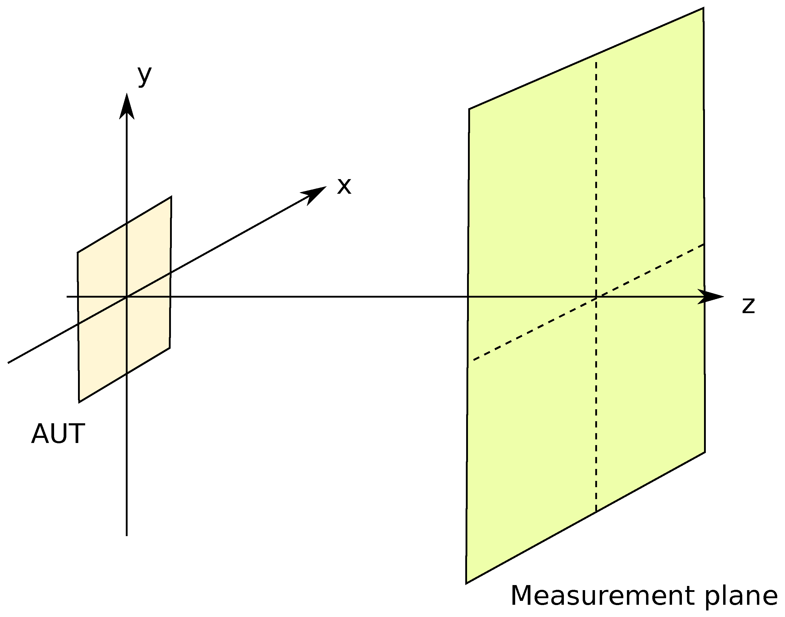
To identify the optimal representation in mean square error sense (i.e., in $L_2$ norm), let us model the AUT as a harmonic electromagnetic source placed in a domain D (see Figure 1). The field, observed on the plane Ω (supposing not intersecting D) is given by [7,14]

$$\begin{array}{c}\hfill \mathbf{E}\left(\mathbf{r}\right)={\int }_D\mathbf{G}(\mathbf{r},{\mathbf{r}}^{\prime })·\mathbf{J}\left({\mathbf{r}}^{\prime }\right)d{\mathbf{r}}^{\prime }\end{array}$$

(1)

where $\mathbf{r}\in \mathsf{\Omega }$, $\mathbf{J}$ is the source current density, $\mathbf{G}$ is the dyadic free space Green’s function [1] and the dot denotes the matrix-vector product.

Following the approach outlined in [7,14], we recast the problem in functional spaces. We consider $\mathbf{J}$ as an element $\overline{x}$ of the set X and $\mathbf{E}$ an element $\overline{y}$ of the set Y, while we call $\mathcal{A}:X\to Y$ the radiation operator mapping X onto the set Y, whose elements are the electric field $\mathbf{E}$ on the measurement plane $\mathsf{\Omega }$. The radiation operator $\mathcal{A}$ is completely continuous (called also compact) [15] (p. 234). In the following discussion, we suppose that the currents and the fields belong to separable Hilbert spaces equipped with $L_2$ norm. Furthermore, the set of the currents is supposed to be bounded with unit radius, i.e., $\parallel x\parallel <1\forall x\in X$.

Let us consider the adjoint of $\mathcal{A}$, denoted as ${\mathcal{A}}^{+}$. The operators $\mathcal{A}{\mathcal{A}}^{+}$ and ${\mathcal{A}}^{+}\mathcal{A}$ are non-negative, compact self-adjoint operators in X and Y, respectively, and admit a countable infinite set of positive eigenvalues, $\{{\sigma }_1\ge {\sigma }_2\ge \dots \}$, that are the same for the two operators and have same multiplicity for the two operators. Using the well know spectral representation of a compact, self-adjoint operator [16] (p. 14, Equation (21)), we have

$$\begin{array}{c}\hfill \mathcal{A}{\mathcal{A}}^{+}{u}_k={\sigma }_k^2{u}_k\end{array}$$

(2)

$$\begin{array}{c}\hfill {\mathcal{A}}^{+}\mathcal{A}{v}_k={\sigma }_k^2{v}_k\end{array}$$

(3)

where $v_k$ and $u_k$ are called left and right singular functions. The compactness of the operator implies that ${lim}_{k\to \infty }{\sigma }_k=0$. The $span(v_1,v_2,\dots )$ is an orthonormal basis for the null space of $\mathcal{A}$, called the subspace of visible objects since it contains all the elements of X that are “observable” in Y, while the $span(u_1,u_2,\dots )$ is an orthonormal basis of the orthogonal complement of the null space of ${\mathcal{A}}^{+}$, i.e., the closure of the subspace of the images of the “visible” objects. The set $({\sigma }_k,u_k,v_k)$ with $k=1,\dots \infty$, is called the singular system of $\mathcal{A}$.

Consequently, it is possible to obtain the following shifted eigenvalue problem:

$$\begin{array}{c}\hfill \mathcal{A}{v}_k={\sigma }_k{u}_k\end{array}$$

(4)

$$\begin{array}{c}\hfill {\mathcal{A}}^{+}{u}_k={\sigma }_k{v}_k\end{array}$$

(5)

By expanding $x\in X$ using the $\left\{v_k\right\}$ basis, from Equation (4), we obtain [16] (p. 14, Equation (23))

$$\begin{array}{c}\hfill \mathcal{A}x=\sum _{k=0}^{\infty }{\sigma }_k\langle x,v_k\rangle u_k\end{array}$$

(6)

where $\langle ·\rangle$ denotes the inner product and $x\in X$.

From Equation (6), we have

$$\begin{array}{c}\hfill \langle \mathcal{A}x,u_k\rangle ={\sigma }_k\langle x,v_k\rangle \end{array}$$

(7)

which is a simple proportionality between the inner product between x and the kth singular function $v_k$ and the inner product between the image of x and the kth singular function $u_k$. From a geometrical perspective, the operator $\mathcal{A}$ maps the unit $L_2$-norm ball into an hyperellipsoid, whose kth semi-axis length is equal to the kth singular value of the Hilbert–Schmidt decomposition of the $\mathcal{A}$ operator.

Since the singular values ${\sigma }_k$ tend to zero for $k\to \infty$, the length of the semi-axes of the hyperellipsoid tend to zero, and the operator $\mathcal{A}$ maps a bounded set X into a (pre-)compact set Y. In practice, we can represent the elements of Y within any desired precision considering a finite-dimensional subspace. Consequently, it is of interest to identify the subspace having the minimum dimensionality assuring that the ($L_2$) approximation error for any element of Y is not larger than a desired quantity. A subspace having this property is called an optimal subspace and its dimensionality is called the Kolmogorov n-width (or also Kolmogorov n-diameter) of Y. The n-width turns out to be equal to the number of singular values above the approximation level plus one, while $span(u_1,u_2,\dots ,u_{n-width})$ is an optimal basis [17] (Chap. 31).

Note that in finite-dimensional Euclidean spaces the linear operator can be represented by a matrix $\mathbf{A}$ and the Hilbert–Schmidt expansion becomes the well known Singular Value Decomposition (SVD) of a matrix [18] (Chap. 8).

From the point of view of the energy concentration, the Hilbert–Schmidt transformation concentrates the energy in the fewesr coefficients for any ($L_2$) desired approximation error. The number of basis, N, is finite for any (not null) degree of approximation, and turns out to be practically equal to the number of singular values greater than the required approximation error [19] (p. 6, Theorem 2).

Consequently, the Hilbert–Smith decomposition allows obtaining both the optimal basis function to represent the field on the measurement plane $\mathsf{\Omega }$ (i.e., the right singular functions) and the number of basis required to represent the field within a given approximation, which is equal to the number of singular values above the noise level plus one. This number, called the Number of Degrees of Freedom (NDF) of the electromagnetic field [9] (p. 921), is also the lower bound of the number of measurements required to represent the field within the required approximation.

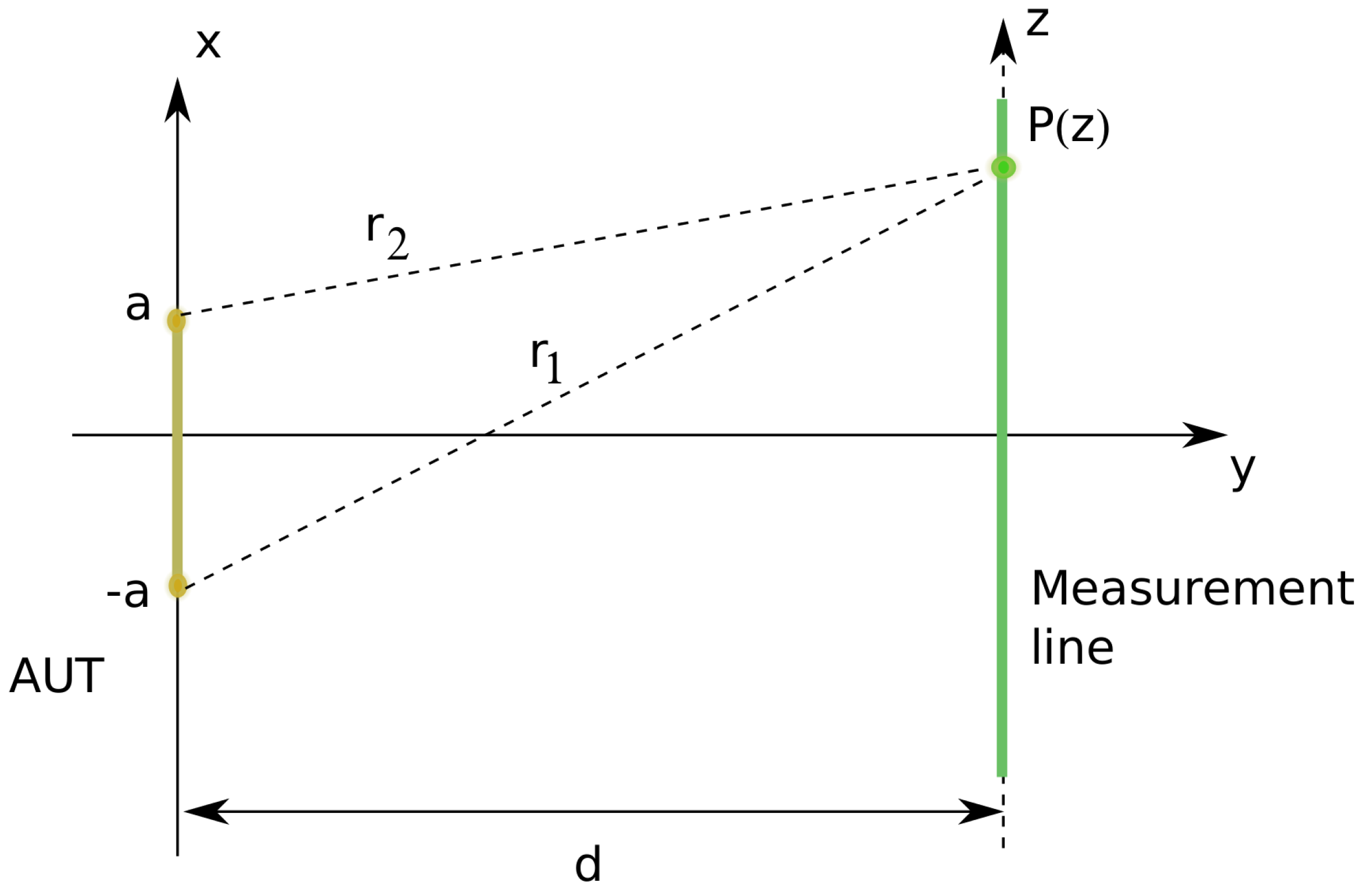
As an example, let us consider a continuous radiating line having length $2a=10\lambda$ (Figure 2). The near-field is measured along a line parallel to the AUT at a distance $d=10\lambda$ from the source.

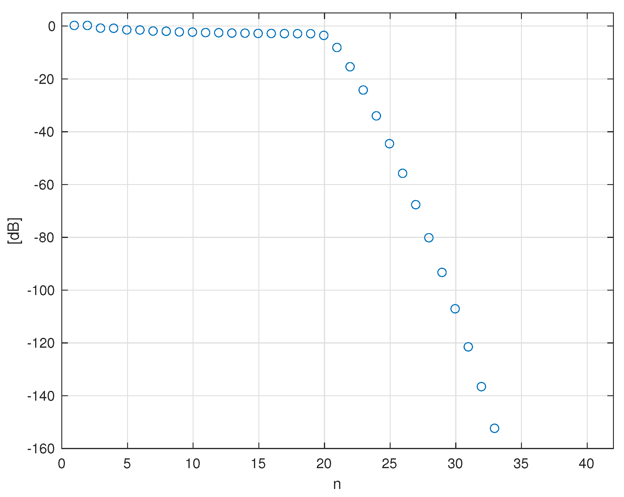
The singular values of the radiation operator normalized to the first one are plotted in Figure 3. The figure shows a knee at the 21st singular value, after which the amplitude of the singular values rapidly decrease to zero. In practice, 21 right singular functions are sufficient to interpolate the field with a high accuracy. Consequently, the number of measurements required to estimate the field configuration using a linear representation is not lower than 21.

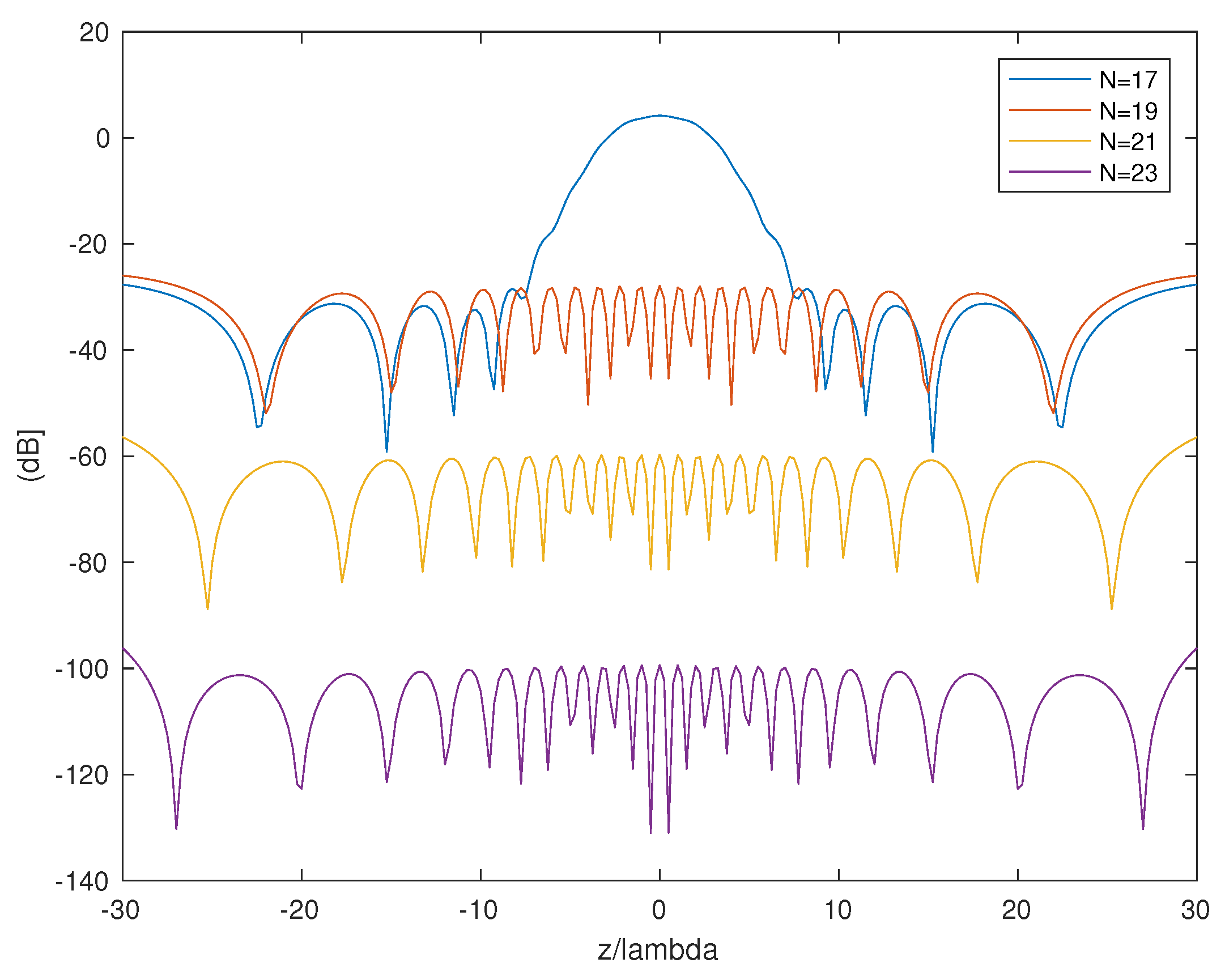
In Figure 4, the error [dB] of the interpolated field considering $N=17,N=19,N=21,N=23$ basis functions is plotted, confirming the good precision of the interpolation using $N=21$.

It is worth noting that the method allows identifying a lower bound in the case of absence of other information on the source but its dimension and shape [20]. Introduction of further a priori information on the source can give linear representations with a lower number of samples.

We use this optimal representation as benchmark to evaluate the sampling techniques. In fact, an array of $\lambda /2$ equispaced elements is basically equivalent to a continuous electromagnetic source in terms of set of radiated field [9]. Accordingly in the following, we consider a linear array of $\lambda /2$ equispaced elements, and we compare the number of samples required to represent the field with the lower bound obtained in this section.

3. Standard Sampling Representation in Planar Near-Field Measurement Systems

The standard sampling representation of the field in planar NF measurements takes advantage of the (almost) finite support of the spectrum of the field [2,4,21].

Let us consider the field the $\mathbf{E}(x,y,z)$ radiated by an electromagnetic source placed at $z=0$ plane and observed on a planar observation surface $\mathsf{\Omega }$ at distance z from the source (Figure 1). The tangent components of the field on the plane

$$\begin{array}{c}\hfill {\mathbf{E}}_t(x,y,z)=E_x(x,y,z)\widehat{x}+E_y(x,y,z)\widehat{y}\end{array}$$

(8)

can be expanded in the plane waves spectrum $\tilde{\mathbf{E}}(k_x,k_y)$ [1] (Ch. 16 p. 856), where

$$\begin{array}{c}\hfill \tilde{\mathbf{E}}(k_x,k_y)={\int }_{-\infty }^{\infty }{\mathbf{E}}_t(x,y,z)exp\left[j(k_{x}x+k_{y}y)\right]\end{array}$$

(9)

obtaining the following Fourier Transform relationship [1] (Ch. 16 p. 856)

$$\begin{array}{c}\hfill \mathbf{E}(x,y,z)=\frac{1}{2\pi }{\int }_{-\infty }^{\infty }\left(\mathbf{I}-\frac{\mathbf{k}}{k_z}\widehat{z}\right){\tilde{\mathbf{E}}}_t(k_x,k_y)exp\left[k_{z}z\right]exp[-j(k_{x}x+k_{y}y)]\end{array}$$

(10)

where $\mathbf{I}$ is the identity matrix and $\mathbf{k}=k_x\widehat{x}+k_y\widehat{y}+k_z\widehat{z}$ is the wavenumber vector. This is basically the Fourier Transform of the function $\mathbf{F}(k_x,k_y,z)={\tilde{\mathbf{E}}}_t(k_x,k_y)exp\left[k_{z}z\right]$.

We recall that $k_x^2+k_y^2+k_z^2={\beta }^2$, where $\beta =2\pi /\lambda$, $\lambda$ is the free space wavenumber. The domain associated to $k_x^2+k_y^2\le {\beta }^2$ is called visible domain. Outside this range, we have that $k_z^2={\beta }^2-k_x^2-k_y^2<0$ and hence the $\tilde{\mathbf{E}}(k_x,k_y)exp[-j{k}_{z}z]$ exponentially decays with the distance z. Consequently, the function $F(k_x,k_y,z)$ is basically concentrated in the visible domain, i.e., in the circle inscribed in the square limited by $|k_x|<\beta$ and $|k_y|<\beta$, and hence it is essentially a band limited function. It is consequently possible to use the Shannon–Whittaker series representation for band limited functions, sampling the field according to the Nyquist sampling step $\pi /w$ where w is the (spatial) angular bandwidth of the field. In our specific case, $w=\beta$, obtaining [1] (Chap. 16 p. 856)

$$\begin{array}{c}\hfill {\mathsf{\Delta }}_x=\frac{\pi }{w}=\frac{\pi }{2\pi /\lambda }=\frac{\lambda }{2}\end{array}$$

(11)

$$\begin{array}{c}\hfill {\mathsf{\Delta }}_y=\frac{\pi }{w}=\frac{\pi }{2\pi /\lambda }=\frac{\lambda }{2}\end{array}$$

(12)

Summarizing, under the hypothesis of negligible value of the plane wave spectrum outside the visible range, the field can be represented by the Shannon–Whittaker sinc series using a uniform $\lambda /2$ sampling step for data acquisition:

$$\begin{array}{c}\hfill E_x(x,y,z)=\sum _m\sum _n{E}_x(x_m,y_n,z)g_{m,n}(x,y)\end{array}$$

(13)

$$\begin{array}{c}\hfill E_y(x,y,z)=\sum _m\sum _n{E}_y(x_m,y_n,z)g_{m,n}(x,y)\end{array}$$

(14)

where $g_{m,n}(x,y)=sinc\left(w(x-x_m)\right)sinc\left(w(y-y_m)\right)$ are the basis functions of the representation, $sinc\left(x\right)=sin\left(x\right)/x$, and $(x_m,y_n)$ are the sampling positions.

Under the hypothesis that the source is not superdirective, the above sampling strategy has an important advantage: it is a “universal”, linear representation, i.e., the field is represented by a linear combination of basis function that do not depend on the specific source. In fact, non-superdirective sources are characterized by negligible value of the plane wave spectrum outside the visible range. It is worth recalling that highly superdirective sources cannot be built, and consequently the above representation can be used in any practical applications. However, it can be noted that it requires, at least theoretically, an infinite number of samples to represent the field on an unbounded surface. This is an indication of a high redundancy of this representation, which is a consequence of the “fixed” basis function and sampling step used.

As an example, an AUT consisting of a linear array of 21 point-like elements having unit excitation with inter element distance equal to $\lambda /2$ is considered (Figure 2). This array has the same length of the continuous source discussed in the example reported in the previous section. The near-field is measured along a line parallel to the AUT at a distance $d=10\lambda$ from the source. The position along the observation line is denoted as z and is normalized to the wavelength.

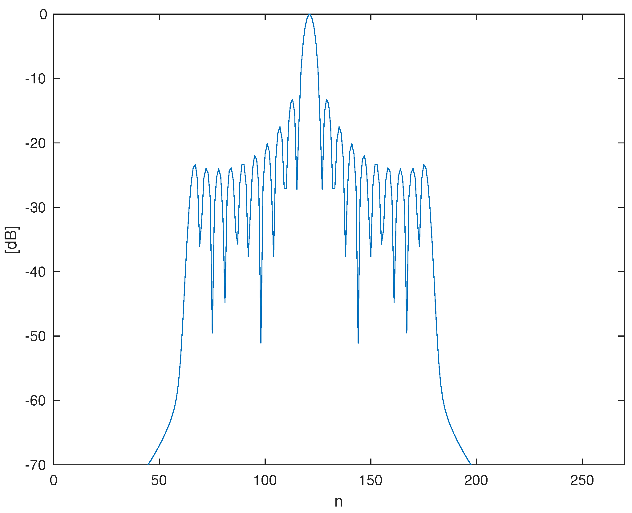
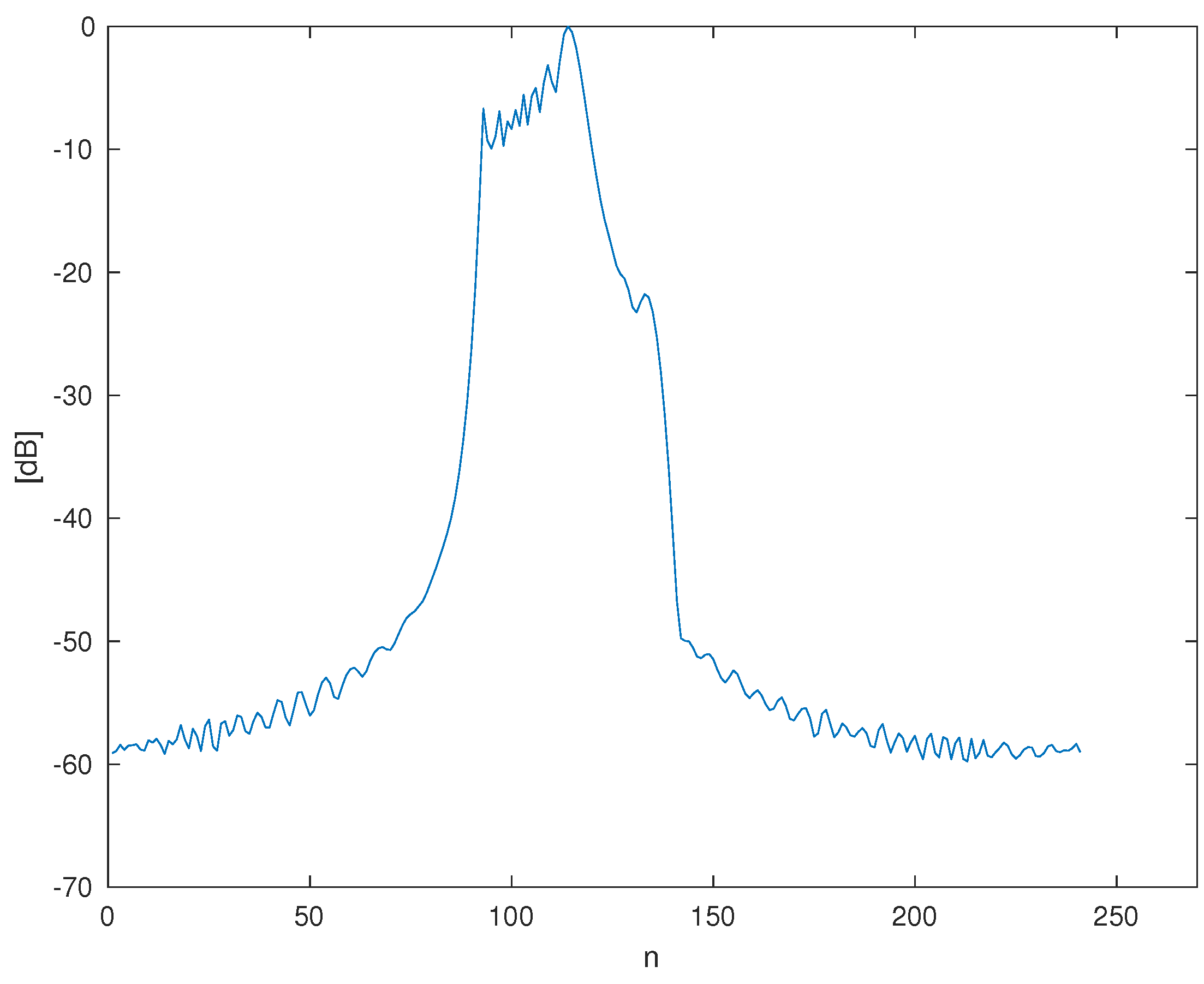
In Figure 5, the amplitude of the Fourier Transform of the field along the observation line is drawn, confirming the concentration of the spectrum in a limited range, that coincides with the visible range.

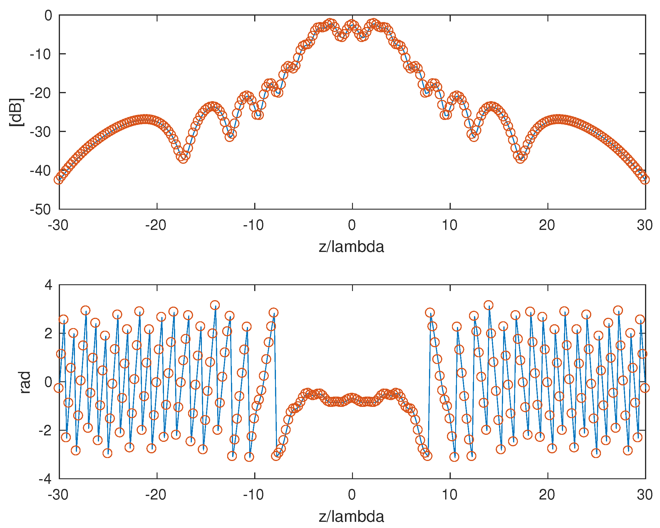
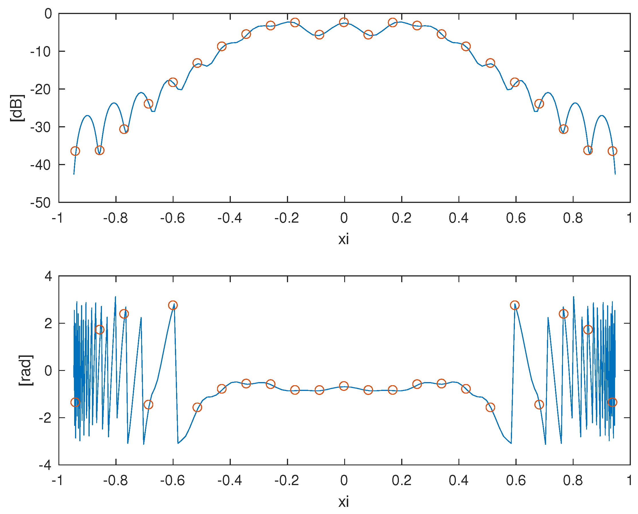
The field radiated by the array and observed along the line is plotted in Figure 6 (top: amplitude in dB; bottom: phase in radiants). The sampling positions are plotted as circles.

The plot shows that 121 samples fall inside the observation range $(-30\lambda ,30\lambda )$. This is a quite large number of samples compared to the lower bound determined in the previous section.

4. The Minimum Redundant Sampling

Minimum Redundant Sampling is a powerful technique developed in the 1990s by Bucci and co-workers. The method can handle many different antenna shapes as well as near-field configurations. The mathematical details are reported in [8,9,11], while experimental validation of the technique is reported in [10]. Extension of the technique to time-domain planar near-field system is reported in [22,23]. In this paper, the technique is introduced using an intuitive approach that clarifies the physics at the basis of the method. The interested reader is invited to refer to [8,9,11] for a rigorous analysis of the technique.

To introduce the method, the analysis is carried out in the time domain. Let us consider a linear source $2a$ long. For sake of simplicity, we suppose that the current density $J(x,t)$ on the source is separable in space domain x and time domain t, i.e., $J(x,t)=g\left(x\right)h\left(t\right)$. We consider the far-field in the point $(R,\theta )$ in a polar system whose origin is in the center of the line source. The field in the observation point is given by the superposition of the retarded contributions of the derivative of the current:

$$\begin{array}{c}\hfill E(\theta ,t)=\frac{{\mu }_0}{4\pi R}{\int }_{-\infty }^{\infty }\frac{\partial J(x,\tau )}{\partial \tau }dx=\\ \hfill =-\frac{{\mu }_{0}c}{4\pi Rsin\left(\theta \right)}{\int }_{-\infty }^{\infty }\frac{\partial g\left(x\right)}{\partial x}h\left(\tau \right)dx\end{array}$$

where $\tau =t-R/c-xsin\theta /c$ is the retarded time and the last expression is obtained by integration by parts.

Let us consider a current density distribution that is constant on $-a\le x\le a$ and is null for $\left|x\right|>a$. The spatial derivative of the current density is the sum of two Dirac delta functionals placed in $x=a$ and in $x=-a$, which represent the “flash points” of the electromagnetic source. The field observed in a point $P\left(z\right)$ is proportional to

$$\begin{array}{c}\hfill E\left(P\right)\propto exp[-j\beta r_1]/r_1+exp[-j\beta r_2]/r_2\end{array}$$

(15)

where, with reference to Figure 2,

$$\begin{array}{c}\hfill r_1=\sqrt{{(x+z)}^2+d^2}\end{array}$$

(16)

$$\begin{array}{c}\hfill r_2=\sqrt{{(x-z)}^2+d^2}\end{array}$$

(17)

and z is the position of the observation point $P\left(z\right)$ on the observation line.

To obtain a simple formula, let us suppose that $r_1\approx r_2$ at the denominator, obtaining

$$\begin{array}{c}\hfill E\left(P\right)\propto 2exp[-j\psi (s\left)\right]cos\left[w\xi \right(s\left)\right]\end{array}$$

(18)

where

$$\begin{array}{c}\hfill \psi \left(z\right)=\beta (r_1+r_2)/2\end{array}$$

(19)

is the mean value of the phase in the point $P\left(z\right)$,

$$\begin{array}{c}\hfill \xi \left(z\right)=\beta (r_2-r_1)/\left(2w\right)\end{array}$$

(20)

is a “parametrization function” of the observation curve (i.e., a nonlinear function of z) and w has the role of a bandwidth.

It is worth noting that the value of the bandwidth w is arbitrary, since the formulas are scaled according to w. The relevant point of this analysis is that choosing the parameterization $\xi \left(s\right)$ the local bandwidth w is constant, i.e., the parameterization compresses the area where the field has lower variation, and expands the area where the field has higher variations.

This property can be analyzed in terms of local variation of the field along the observation point $P\left(z\right)$. Let us linearize $w\xi \left(s\right)$ around $P\left(s\right)$ along the observation line, obtaining $w\left(\xi \right(s\left)\right)ds$. The quantity $w\left(\xi \right(s\left)\right)$ is a spatial “local bandwidth” around P at curvilinear abscissa s. Roughly speaking, we can imagine the local bandwidth as the bandwidth of the field in a “short spatial slot” around $P\left(s\right)$. Basically, the concept of local bandwidth is similar to the Short Time Fourier Transform (STFT) that is widely used in audio signal processing. The transformation $\xi \left(s\right)$ modifies the curve so that the local bandwidth turns out to be constant along the stretched observation curve.

Consequently, the field can be represented along the observation line using the following Shannon–Whittaker series [10] (p. 356, Equation (38)):

$$\begin{array}{c}\hfill E\left(\xi \right)=\sum _k{c}_{k}sinc\left(w(\xi -x{i}_k)\right)exp\left(j\varphi \left(\xi \right)\right)\end{array}$$

(21)

The above simple example, even if not rigorous, shows the physical basis of the method. In practice, there are some “critical” points on the source associated to the radiated field. These points fix the rate of spatial variation of the field around an observation point P, i.e., the “spatial bandwidth” of the field around P. It is interesting to note that the physical mechanism at the base of the method has strong connections to the ones at the basis of the Geometrical Theory of Diffraction [24].

As stressed at the beginning of this section, the above discussion gives only an intuitive explanation of the physical bases of the minimum redundant sampling developed by Bucci and co-workers [8]. The reader is invited to refer to the papers [8,10] for the rigorous analysis of the problem.

Basically, the method is the following one: instead of the field $E\left(z\right)$, the “reduced field” $F\left(z\right)$ is considered; the reduced field is obtained by the field after the extraction of a proper phase function $\psi \left(\xi \right)$ and the introduction of a proper parameterization function $\xi \left(s\right)$ of the observation curve:

$$\begin{array}{c}\hfill F\left(\xi \right)=E\left(\xi \right)exp\left(j\psi \right(\xi \left)\right)\end{array}$$

(22)

The function $F\left(\xi \right)$ is an almost bandlimited function with effective bandwidth w. The functions $\xi \left(z\right)$ and $\psi \left(z\right)$ depend on the shape of the source, and the geometry of the observation plane. The expression of the functions for the main source geometries are reported in [10,11,25,26]. For example, in the case of a simple linear observation curve, the functions are [10] (p. 355, Equations (27) and (28) evaluated for a linear source and a linear observation curve):

$$\begin{array}{c}\hfill \psi \left(z\right)=\pi (r_1+r_2)\end{array}$$

(23)

$$\begin{array}{c}\hfill \xi \left(z\right)=(r_2-r_1)/\left(2a\right)\end{array}$$

(24)

$$\begin{array}{c}\hfill w=2a\end{array}$$

(25)

It is possible to approximate F with a bandlimited function within any degree of approximation considering a slightly larger bandwidth, e.g., $\chi w$, where $\chi$ is a bandlimitation enlargement factor slightly larger than one. The approximation error between F and the $\chi w$ bandlimited version of F rapidly tends to zero with $\chi$ [8] (p. 1451, Equation (43)).

Consequently, the reduced field can be represented as:

$$\begin{array}{c}\hfill F\left(\xi \right)=\sum _{k}F\left({\xi }_k\right)sinc\left(w(\xi -{\xi }_k)\right)+ϵ\left(\chi \right)\end{array}$$

(26)

where $F\left({\xi }_k\right)=E\left({\xi }_k\right)exp\left(j\psi \left({\xi }_k\right)\right)$ are samples ${\xi }_k=n\mathsf{\Delta }\xi$ measured at Nyquist spatial step, equal to $\mathsf{\Delta }\xi =1/\left(2a\chi \right)$ and $ϵ$ is the bandlimitation representation error, which can be reduced to an arbitrarily small value by a proper choice of $\chi$. A value of $\chi$ between 1.1 and 1.2 is generally sufficient to assure a bandlimitation representation much lower than the noise level affecting the measured data.

Finally,

$$\begin{array}{c}\hfill E\left(\xi \right)=exp(-j\psi \left(\xi \right))\sum _{k}E\left({\xi }_k\right)exp\left(j\psi \left({\xi }_k\right)\right)sinc\left(w(\xi -{\xi }_k)\right)+ϵ\left(\chi \right)\end{array}$$

(27)

It turns out that the number of field samples $N=int\left[\right(1+\chi \left)w\right]$ required using the above representation are only slightly larger than the minimum number of samples required in a linear representation (i.e., of the $NDF$) obtained using the method outlined in the previous section.

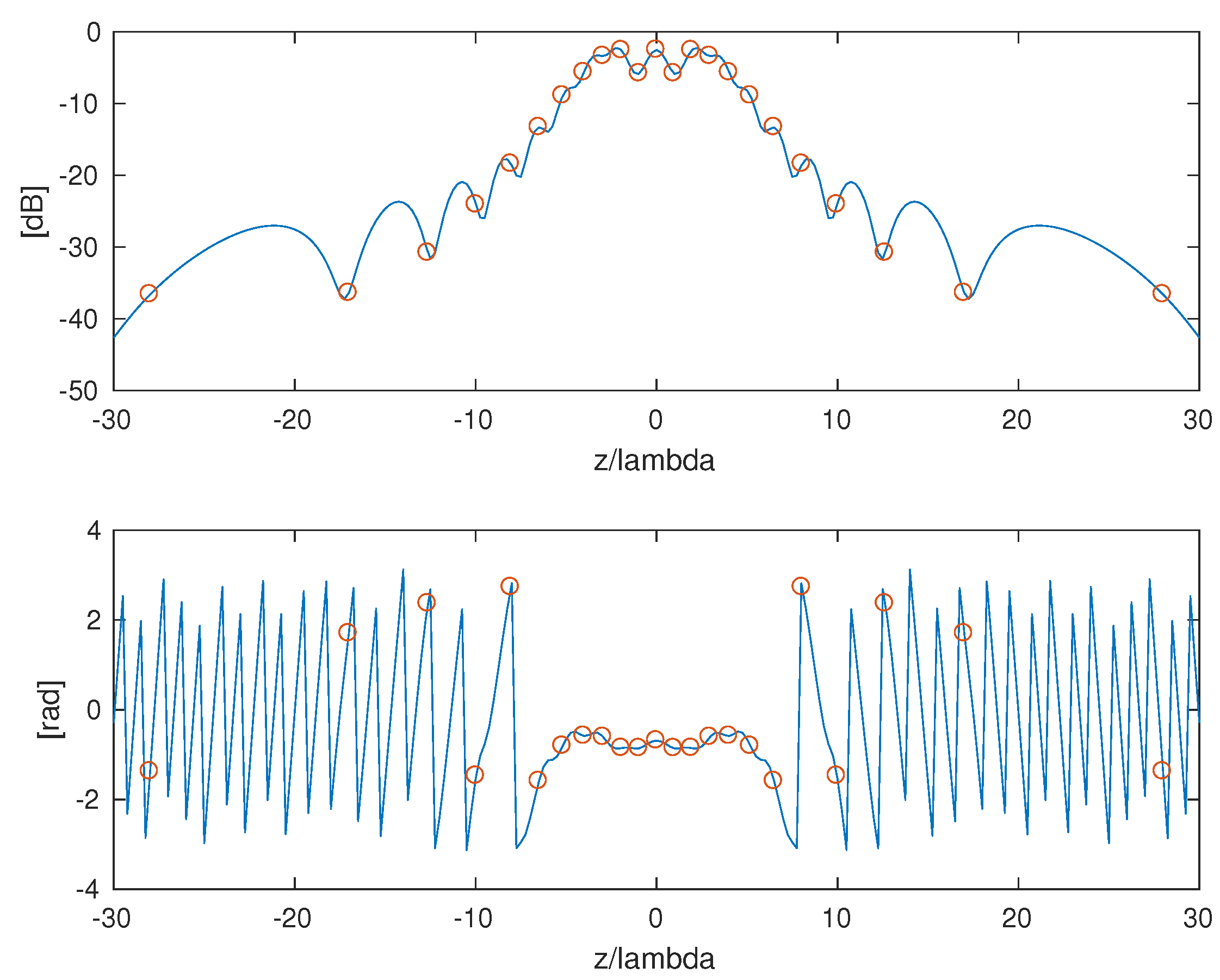
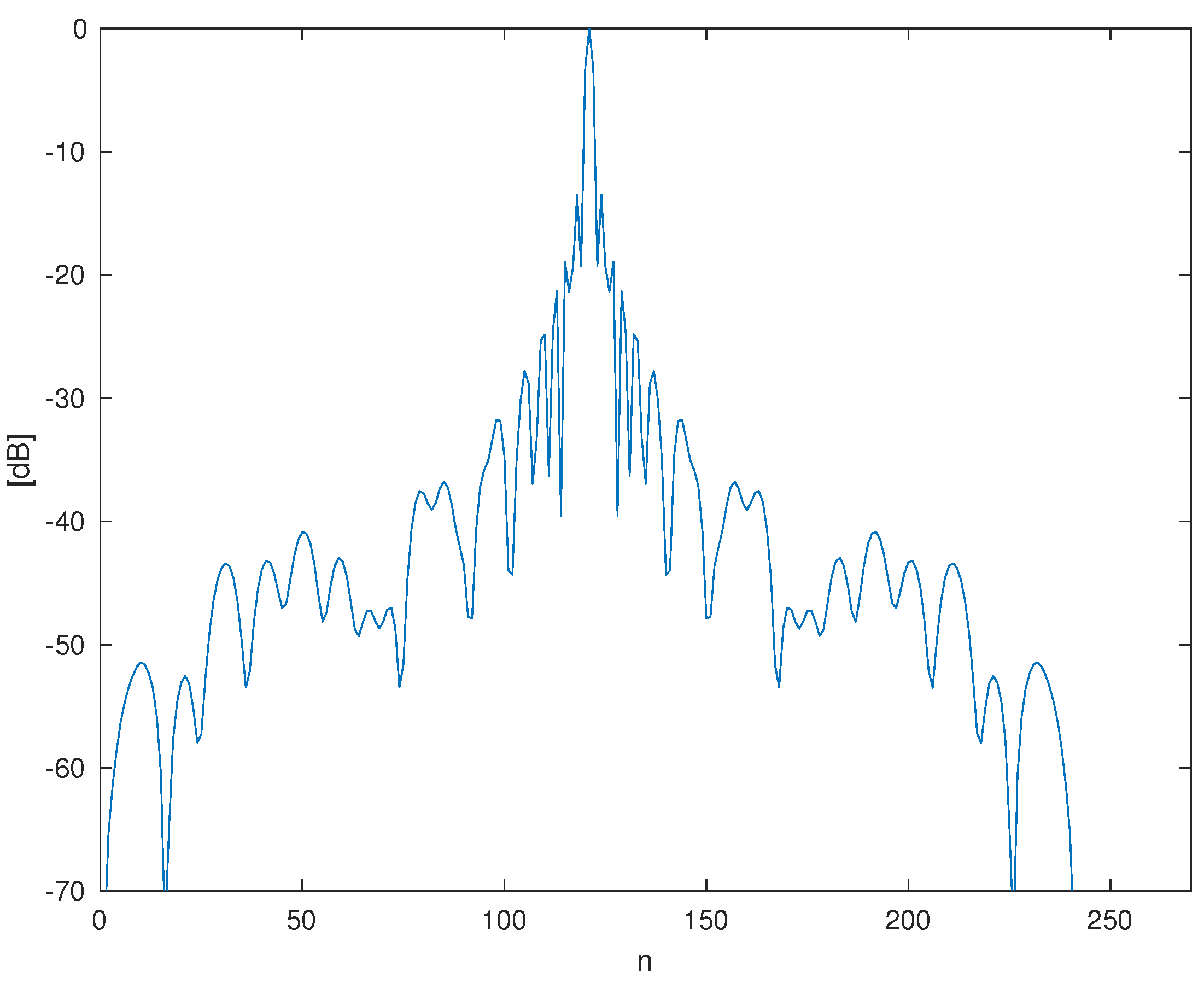
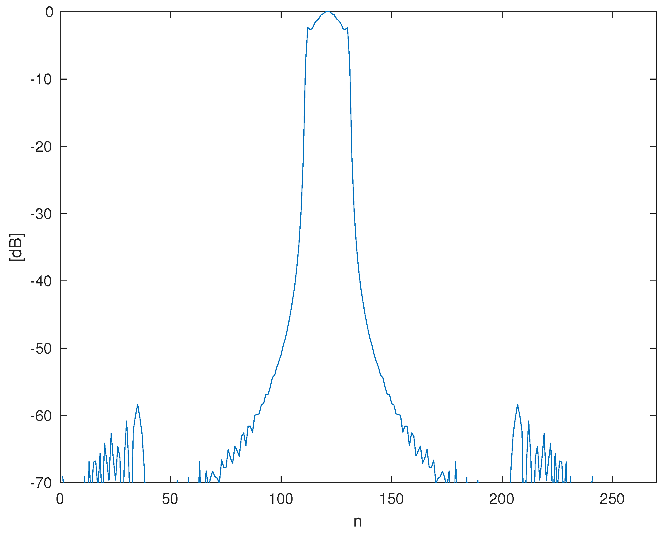
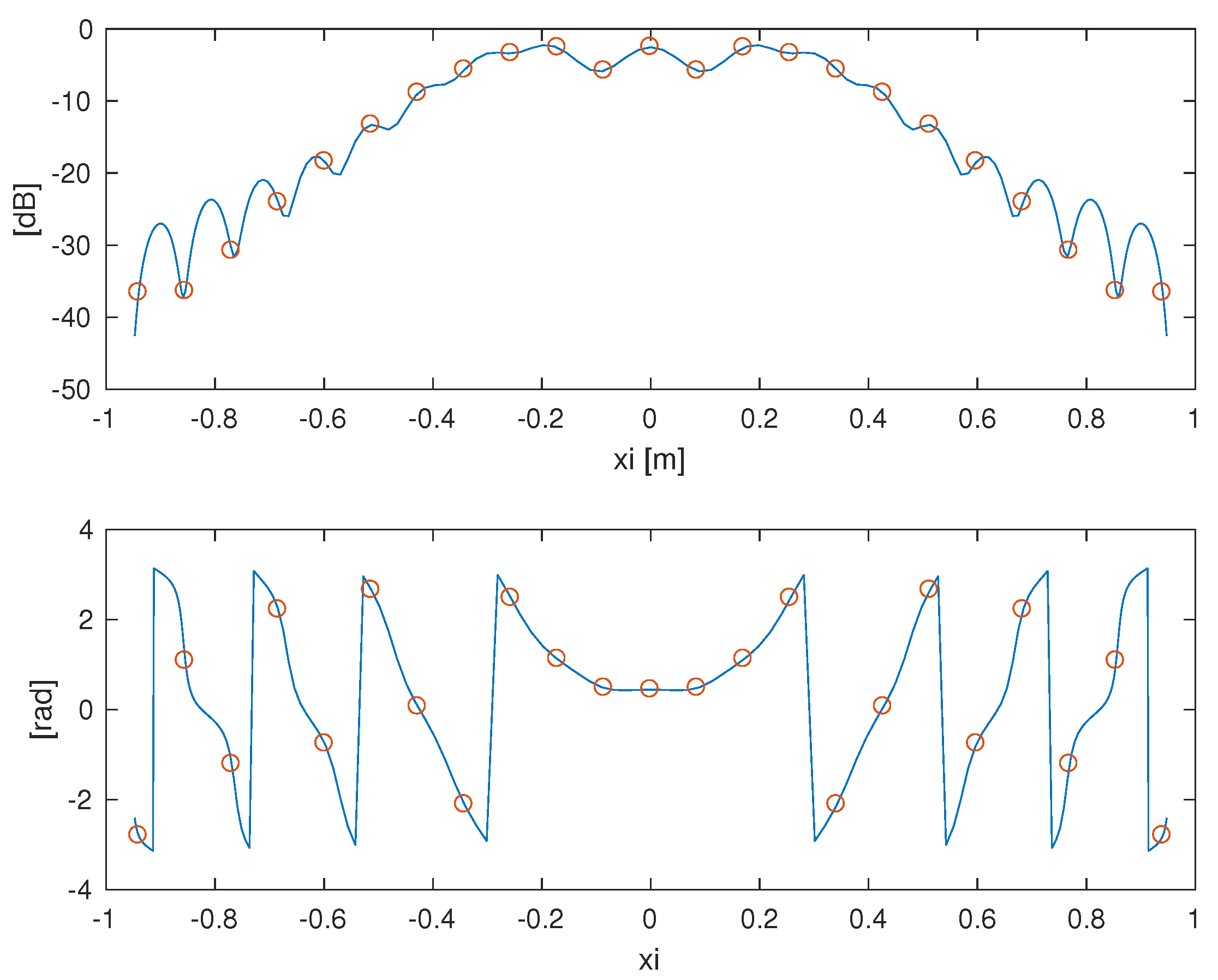
To clarify the method, let us consider the same example regarding a linear array discussed in the previous sections. The field $E\left(z\right)$ (amplitude and phase) along the observation line is plotted as blue curve in Figure 7. The field $E\left(\xi \right)$ (amplitude and phase) is plotted in Figure 8 as blue continuous curve. Note that no phase function extraction has been done at this step. The plot shows a smoother function compared to $E\left(z\right)$, but with a still fast phase variation. The spectrum of $E\left(\xi \right)$ is plotted in Figure 9, showing a quite spread spectrum. Finally, the spectrum of $F\left(\xi \right)$ (i.e., after phase extraction) is shown in Figure 10. The plot confirms the narrow bandwidth of the reduced field. Consequently, the reduced near-field is much smoother, as shown in Figure 11 (amplitude and phase). In the same figure, the samples collected at constant $\mathsf{\Delta }\xi$ step with an oversampling factor $\chi =1.17$ are plotted as circles. The positions of these points on z are shown in Figure 7. We can note that the sampling is uniform in $\xi$ but non-uniform in z. The number of samples required to represent the field in the entire unbounded observation line (i.e.; in the interval $-\infty <z<\infty$ ) is 23, only slightly larger then the minimum possible number that was evaluated in the previous sections, and turned to be 21.

The above representation is of great interest since it gives an almost optimal representation that allows using all the theory of band limited functions developed in the signal processing community with small modifications. As an example of how the theory allows improving the near-field measurement techniques, we consider two practical problems affecting the NF set-ups.

The first problem regards the so-called truncation error [27]. Due to the finite dimension of the scanning surface, the near-field can be measured only on a finite area. The use of truncated data is equivalent to multiplying the data for a window function. Since the FF is obtained from the NF by a Fourier Transform, the effect is an error in the far-field reconstruction and a limitation of the angular region where the far-field is reliably estimated.

Let us suppose for example that the available data are within $-10\lambda <z<10\lambda$. In standard near-field measurements, estimation of the field outside the measurement area requires a huge number of data, since the sampling step is $\lambda /2$. Instead, using the reduced field only six samples (three on the left and three on the right) fall outside the measurement area. They can be estimated from the available measured data using inverse problem techniques with a good accuracy, improving the far-field accuracy [28]. Since the positions of the sampling points required to estimate the field is known in the space around the antenna, it is also possible to collect the missed field in other places that are accessible to the near-field system [29], further improving the far-field estimation.

A further problem that can be handled using MRS is the presence of scattering points in the measurement set-up. In this case, it is possible to exploit the fact that the source must be centered with respect to the $\xi$ and $\psi$ function to reduce the bandwidth. If the source is not centered, the “reduced field” turns to have a larger bandwidth.

As an example, the same linear array considered in the previous examples is shifted of $10\lambda$ with respect to the center of the coordinate system. Consequently, the parameterization and the phase functions are erroneous. The spectrum of $F\left(\xi \right)$ function obtained is shown in Figure 12. This spectrum must be compared with the spectrum in Figure 10. The comparison between the two figures clearly shows that the transformation concentrates the energy of the field in the lower harmonics if the antenna is correctly centered in the reference system, otherwise the energy is spread toward the higher components of the spectrum.

Scattering points are generally placed far form the antenna, so that the most part of their energy is concentrated in the higher components of the spectrum of the reduced field, outside the $(-\chi w,\chi w)$ spatial bandwidth of the source (that is correctly placed in the reference system). Consequently, a simple low-pass filtering of the measured data allows excluding the most part of the energy of the scattering sources affecting the measurement environment [30].

5. Nonlinear Interpolation

The above techniques are based on a linear interpolation of the field. Recently, there is a growing interest toward nonlinear interpolation [31], which in some specific cases allows a decrease of the number of measurements required to interpolate the field.

As an example, let us consider the application of Compressed Sensing/Sparse Recovery to array diagnosis [32]. The goal is to identify possible failures in an array from a small number of measurements.

Let us consider again a uniform linear array of N elements radiating in free space, with inter element distance $d=\lambda /2$, $\lambda$ being the free-space wavelength. We suppose that there are broken elements that do not radiate. The goal is to identify these elements from far-field measurements, hopefully using a small number of measurements. We suppose that the excitations of the failure-free array are available, as well as the far-field radiated by the failure-free array in M measurement points. The failure-free array (i.e., the “gold array”) is denoted as reference array.

Let ${\mathbf{y}}^r\in {\mathbf{C}}^M$ be the vector collecting the far-field of the failure-free array (where the apex r stands for “reference”), and ${\mathbf{x}}^r\in {\mathbf{C}}^N$ the vector of its excitations. The field radiated by the AUT with fault elements is collected in the vector ${\mathbf{y}}^d\in {\mathbf{C}}^M$, while the vector of the excitations of the AUT with fault elements is denoted as ${\mathbf{x}}^d\in {\mathbf{C}}^N$.

Now, we consider the system

$$\mathbf{A}\mathbf{x}=\mathbf{y}$$

(28)

where

$$\begin{array}{c}\hfill \mathbf{x}={\mathbf{x}}^r-{\mathbf{x}}^d\end{array}$$

(29)

$$\begin{array}{c}\hfill \mathbf{y}={\mathbf{y}}^r-{\mathbf{y}}^d\end{array}$$

(30)

are “innovation” vectors and $\mathbf{A}\in {\mathbf{C}}^{M\times N}$ is the radiation matrix relating the excitations to the far-field data. If the number of fault elements S is much smaller than N (as usually happens), we have an equivalent problem involving a highly sparse array, in which only the “fault elements” of the original array radiate.

Sparse problems are characterized by the presence of a large number of null entries (or almost null entries, in which case they are called “compressible problems’) in the unknown vector. The presence of a large number of null entries is a powerful a priori information that can be exploited in the solution of the undetermined linear system.

In the following, the vector $\mathbf{x}$ is called S-sparse if the number of non-null elements is not larger than S. The set of all the S-sparse vectors is called ${\mathrm{\Sigma }}_S$. Our goal is to estimate $\mathbf{x}$ from $\mathbf{y}$.

Following the compressed sensing literature, with abuse of notation, the number of non-null elements is called zero-norm or ${\ell }_0$ norm, of the vector $\mathbf{x}$, and is denoted as ${\parallel \mathbf{x}\parallel }_0$, while the ${\ell }_1$ norm is given by the classic definition

$$\begin{array}{c}\hfill {\parallel \mathbf{x}\parallel }_1:=\sum _{j=1}^N\left|x_j\right|\end{array}$$

(31)

Given a matrix $\mathbf{A}$, the goal is to find the sparsest solution compatible with the measurement vector $\mathbf{y}$, i.e., the solution of the following minimization problem:

$$\begin{array}{c}\hfill arg\underset{x}{min}{\parallel \mathbf{x}\parallel }_{0}s,t,\mathbf{A}\mathbf{x}=\mathbf{y}\end{array}$$

(32)

Unfortunately, no efficient algorithm able to solve the above problem is known. Its solution requires to check all the possible combinations of subspaces whose union gives ${\mathrm{\Sigma }}_S$, with a computational burden exponentially increasing with N.

Instead of minimizing the ${\ell }_0$ norm, it is possible to relax the zero-norm minimization considering $p=1-\mathrm{norm}$, solving the following optimization problem

$$\begin{array}{c}\hfill arg\underset{x}{min}{\parallel \mathbf{x}\parallel }_{1}s.t.\mathbf{A}\mathbf{x}=\mathbf{y}\end{array}$$

(33)

in absence of noise in the data, or the equivalent to the “Ivanov” regularization strategy

$$\begin{array}{c}\hfill arg\underset{x}{min}{\parallel \mathbf{x}\parallel }_{1}s.t.{\parallel \mathbf{A}\mathbf{x}-\mathbf{y}\parallel }_2\le ϵ\end{array}$$

(34)

in presence of noisy data affected by an uncertainty level $ϵ$.

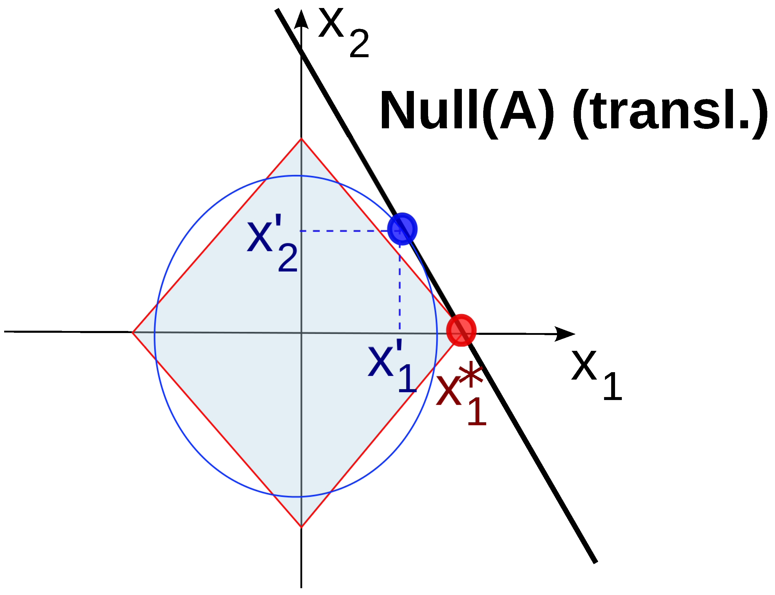
To clarify how the ${\ell }_1$ norm promotes the sparsification of the solution, let us consider a simple geometrical example commonly used to explain ${\ell }_1$ minimization. With reference to a two-dimensional space let us consider $N=2$, $\mathbf{x}=(x_1,x_2)$, $M=1$ and $S=1$. Accordingly, the null space $\mathcal{N}$ is a line. The set of all the solutions of the equation $\mathbf{A}\mathbf{x}=\mathbf{y}$ is the null space translated according to the solution ${\mathbf{x}}^{\ast }=(x_1^{\ast },0)$. The r-radius ball in ${\ell }_1$ is the locus of the points such that $|x_1|+|x_2|=r$ and has a rhombic shape. The solution of the minimization problem is the intersection point between the translated null space of $\mathbf{A}$ and the smallest ${\ell }_1$ ball intersecting the translated null space, as shown in Figure 13.

The figure shows also that generally the sparse solution $(x_1^{\ast },0)$ is not the solution at minimum distance from the origin. This is the reason at the basis of the failure of the least squares approach, given by the point $(x_1^{\prime },x_2^{\prime })$ (drawn in blue in the figure).

As in any inverse problem, an important issue is the stability of the linear problem involving the matrix $\mathbf{A}$, that plays the role of the sensing matrix of the sparse problem [33]. In particular, in our case, we are interested in considering the stability of the solution restricted to set of sparse vectors $\mathbf{x}\in {\mathrm{\Sigma }}_S$, or equivalently the stability of all the possible submatrices of $\mathbf{A}$ obtained by picking up S columns of $\mathbf{A}$. This approach is at the basis of the Restricted Isometry Property, or $RIP$, introduced by Candes and Tao [34].

A (properly normalized) matrix $\mathbf{A}$ is said to satisfy the Restricted Isometry Property ($RIP$) with $RIP$ constant ${\delta }_S$ (${\delta }_S\in (0,1)$) if ${\delta }_S$ is the smallest constant such that for every $\mathbf{x}\in {\mathrm{\Sigma }}_S$ (i.e., for any $S-$sparse vector):

$$\begin{array}{c}\hfill (1-{\delta }_S)\le \frac{{\parallel \mathbf{A}\mathbf{x}\parallel }_2^2}{{\parallel \mathbf{x}\parallel }_2^2}\le (1+{\delta }_S)\end{array}$$

(35)

Intuitively, $RIP\left({\delta }_S\right)$ measures “how well” every set of S columns of $\mathbf{A}$ forms approximately an orthonormal system. Equivalently, $RIP\left({\delta }_S\right)$ requires that the eigenvalues of any ${\mathbf{A}}_S^H{\mathbf{A}}_S$ matrix (where ${\mathbf{A}}_S$ matrix is obtained by picking up S colums of $\mathbf{A}$) are within $1-{\delta }_S$ and $1+{\delta }_S$ so that all the ${\mathbf{A}}_S^H{\mathbf{A}}_S$ are “close” to an isometry. Broadly speaking, the smaller is ${\delta }_S$, the more stable is the linear mapping involving S-sparse vector. We can note that this stability condition must be valid not for any $\mathbf{x}\in C^N$ but only for the restricted set of vectors belonging to ${\mathrm{\Sigma }}_S$. In practice, this condition is a restricted stability condition.

We recall also that the difference vector of two elements belonging to ${\mathrm{\Sigma }}_S$ does not generally belong to ${\mathrm{\Sigma }}_S$ (and in fact ${\mathrm{\Sigma }}_S$ is not a linear space), but belongs to ${\mathrm{\Sigma }}_{2S}$. Consequently, the condition the $RIP$ usually refers to ${\mathrm{\Sigma }}_{2S}$ space.

The interest toward the $RIP$ condition comes from the seminal papers of Tao and Candes [34] and Donoho [12] that discuss the equivalence between ${\ell }_0-{\ell }_1$ minimization equivalence [35] (p. 5411).

In particular, if $\mathbf{x}$ is the $S-$sparse unknown vector and ${\mathbf{x}}^{\ast }$ the solution of the ${\ell }_1$ minimization, the condition $RIP\left({\delta }_{2S}\right)<c$ assures that in case of data affected by $ϵ$-bounded 2-norm uncertainty we have $\parallel {\mathbf{x}}^{\ast }{-\mathbf{x}\parallel }_2\le C_0ϵ$ [12,34] for some constant $C_0$. The first evaluation of c was provided by Candes for ${\delta }_{2k}$ ($c=\sqrt{2}-1$,34] (Theorem 1.1) ), but the research on this subject is very active, and conditions on ${\delta }_k$ are also available [36] (${\delta }_k$ > 0.307, Equation (5)). These bounds are obtained considering real vectors. Sparse vectors can be treated as real vectors having double length.

Similar theorems have been obtained also in the case of “compressible vectors”, i.e., vectors that are not rigorously sparse, but whose elements, sorted in decreasing magnitude, quickly decay [34]. For such vectors, under the hypothesis that $RIP\left({\delta }_{2S}\right)<\sqrt{2}-1$, we have

$$\begin{array}{c}\hfill \parallel {\mathbf{x}}^{\ast }{-\mathbf{x}\parallel }_2\le C_0{\parallel \mathbf{x}-{\mathbf{x}}_S\parallel }_1/\sqrt{S}+C_1ϵ\end{array}$$

(36)

for some constant $C_0$, where ${\mathbf{x}}_S$, called S-best approximation, is the vector $\mathbf{x}$ with all but the largest S components set to zero.

Sampling strategies verifying the $RIP$ conditions in array diagnosis are available for far-field measurements. In Reference [37], N angular measurement directions equispaced in the $u=sin\left(\theta \right)$ space are selected to obtain an unitary (normalized) radiation matrix $\mathbf{U}$ whose $(m,n)$ entry is

$${\left[\mathbf{U}\right]}_{m,n}=\frac{1}{\sqrt{N}}exp\left(-j2\pi \frac{mn}{N}\right)$$

(37)

Starting from $\mathbf{U}$, the radiation matrix $\mathbf{A}$ is obtained selecting M rows uniformly at random among the N rows of the discrete Fourier matrix $\mathbf{U}$. The radiation matrix turns out to be a random partial Fourier matrix, and consequently verifies the so-called concentration inequality [38]

$$\begin{array}{c}\hfill {Prob\left(\right|\parallel \mathbf{A}\mathbf{x}\parallel }_2^2-{\parallel \mathbf{x}\parallel }_2^2{|\ge \delta \parallel \mathbf{x}\parallel }_2^2)\le 2e^{-c{\delta }^{2}M}\end{array}$$

(38)

where $0<\delta <1$, c is a constant and Prob stands for probability. Such an inequality assures that $\mathbf{A}$ verifies also $RIP\left({\delta }_S\right)$ with probability exceeding $1-ϵ$, provided that $M\ge C{\delta }^{-2}(Slog(N/M)+log\left({ϵ}^{-1}\right))$ for some C [38] (Theorem 3.6, p. 18), where ${\delta }_S\le \delta$.

Similar approach have also been proposed in near-field measurements [31]. More recently, non-random strategies assuring the RIP property have also proposed [39].

The CS/SR technique has been applied in many near-field and far-field research, and experimental results [40,41,42] confirm the effectiveness of the techniques.

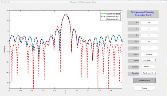
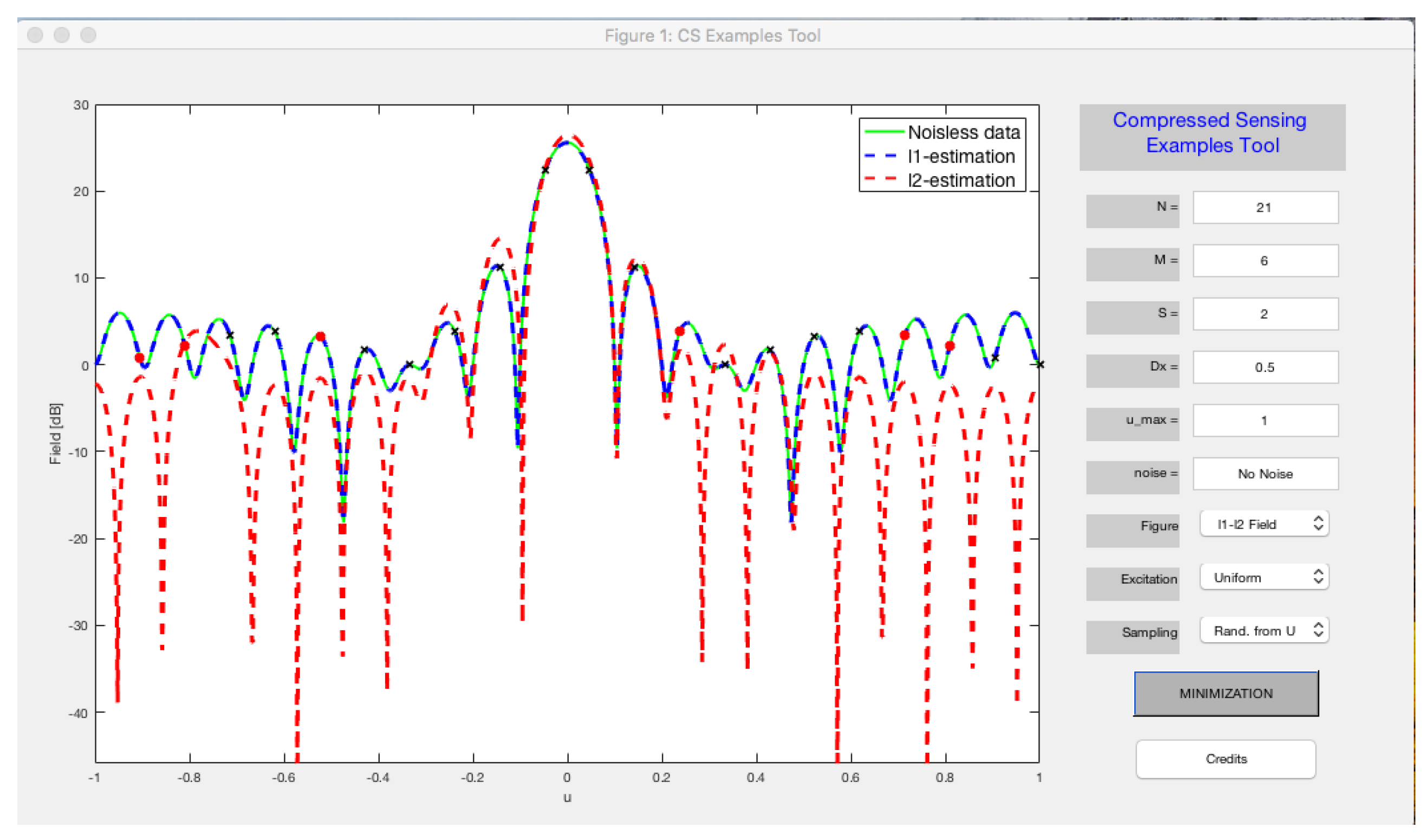
As an example, the same 21-element ULA considered in the previous sections is analyzed. A number of $S=2$ failure and $M=6$ measurements are considered. Despite the quite low number of measurements, the field is correctly reconstructed, as shown in Figure 14 (blue curve, covering the black curve representing the exact field in the case of two failures). In the same figure, the result obtaining using a linear estimation from the six measured data is plotted as red dashed curve, showing poor performance.

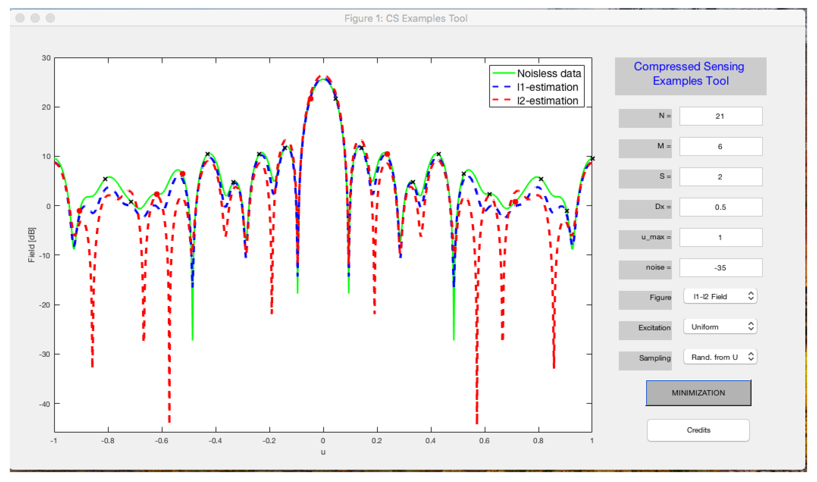
The effectiveness of the technique is confirmed also in presence of data corrupted by noise, as confirmed in Figure 15.

The above figures have been obtained from the free program “CS Examples Tool”. Interested readers can download the program [13] reported in Appendix A and carry out their own investigation on the technique. A short description of the program is reported in Appendix A.

6. Conclusions

In this paper, some sampling techniques for near-field antenna measurements have been discussed.

Table 1. Comparison between sampling techniques for the measurement geometry used in the examples reported in this paper.

Sampling Technique	Number of Samples	A Priori Information	Computational Complexity
Standard $\lambda /2$ sampling	121	-	very low
Minimum redundant sampling ($\chi =1.17$)	23	Shape and size	low
Lower bound using linear representation	21	shape and size	High
Sparse representation (S = 2 failures)	6	Sparse sources	High

shows a comparison among some parameters of interest in practical applications with reference to the measurement geometry considered in the examples discussed in this paper (21-element linear array $\lambda /2$ equispaced and $(-30\lambda ,30\lambda )$ long observation line).

Standard $\lambda /2$ sampling method can be applied to any (non-superdirective) source without needing specific a priori information on the electromagnetic source (of course apart from the frequency). However, the number of samples (second row) is significantly higher than the other technique. Regarding the computational burden required to interpolate the field in a denser lattice, let us consider the “best case”, i.e., the interpolation of the measured data on $N=2^p$ equispaced points, where p is an integer. In this case, the interpolation can be obtained by Fast Fourier Transform (FFT) of the zero padding data vector, and requires a time proportional to $M^{″}log{M}^{\prime }$ where $M^{\prime }$ is the number of interpolation positions.

The minimum redundant sampling method requires a number of samples almost an order of magnitude smaller than the $\lambda /2$ equispaced strategy. Its use requires some information about the source (the general shape and the size) that is easily available. The method can be applied to any (non-superdirective) source with a proper choice of the oversampling factor $\chi$ as indicated in [9]. The samples are non-uniformly placed on the observation plane, and consequently the interpolation on a uniform lattice requires the use of the sampling series with sinc kernel. However, the use of self-truncating functions instead of standard sinc functions, as done in [9], allows using only few samples, e.g., Q, around the interpolation position. Consequently, the computational complexity is proportional to $Q{M}^{\prime }$, where $M^{\prime }$ is the number of interpolation positions.

The Hilbert–Smith decomposition of the radiation operator is reported in the paper to identify the lower bound of the number of measurements, and is not a “practical” sampling method. The required a priori information is the same of the minimum redundant sampling method, with the difference that it is possible to include a much more detailed description of the geometry of the source. In the example reported in this paper, the same a priori information are used for both the methods. The number of samples (21) is only slightly smaller than the minimum redundant sampling method. The computational burden is high, since it basically requires a Singular Value Decomposition. For example, the R-SVD algorithm gives a computational burden of $6M{N}^2+20N^3$ [18] (Chap. 5, p. 254), where N is the number of radiating elements in the case of array or the number of elements in which the source is discretized in the case of continuous source.

Finally, CS/SR requires a number of samples that depends on the sparsity of the unknown vector, and hence on the number of failures in array diagnosis. A “rule of the thumb” is that a number of measurements between 3 and 4 times the number of failures is sufficient to obtain an accurate reconstruction. The method uses the sparseness of the unknown vector to reconstruct the field, and hence requires stronger a priori information. Evaluation of the computational burden is extremely complex, since it depends on the specific algorithm used. For example, CVX allows solving array of several hundreds of elements in less than 10 min. The use of other optimized algorithms allows a further decrease of the computation time.

As noted in the Introduction, electromagnetic sampling is an active field of research, and many new approaches and strategies are under development. These approaches include “blind” interpolation without using any a priori information on the source [43,44], the reduction of the number of measurements using numerical simulations of the AUT [45,46], and the use of adaptive sampling [47]. As a last observation, the optimal linear representation of the field has applications not only in near-field measurements, but in a large number of areas of interest in communication systems, for example MIMO systems [48] and secure wireless communications [49].

References

- Balanis, C. Antenna Theory Analysis and Design; Wiley: New York, NY, USA, 2015. [Google Scholar]
- Wang, J.H. An Examination of the Theory and Practices of Planar Near-Field Measurement. IEEE Trans. Antennas Propag. 1988, 36, 746–753. [Google Scholar] [CrossRef]
- Newell, A.C. Error Analysis Techniques for Planar Near-Field Measurements. IEEE Trans. Antennas Propag. 1988, 36, 756–768. [Google Scholar] [CrossRef]
- Slater, D. Near Field Antenna Measurements; Artech House: New York, NY, USA, 1991. [Google Scholar]
- Johnson, R.; Ecker, H.; Moore, R. Compact range techniques and measurements. IEEE Trans. Antennas Propag. 1969, 17, 568–576. [Google Scholar] [CrossRef]
- Yaghijan, A. An overview of near-field antenna measurements. IEEE Trans. Antennas Propag. 1986, 34, 30–45. [Google Scholar] [CrossRef] [Green Version]
- Migliore, M.D. On electromagnetics and information theory. IEEE Trans. Antennas Propag. 2008, 56, 3188–3200. [Google Scholar] [CrossRef]
- Bucci, O.M.; Franceschetti, G. On the spatial bandwidth of scattered field. IEEE Trans. Antennas Propag. 1987, 36, 1445–1455. [Google Scholar] [CrossRef]
- Bucci, O.M.; Franceschetti, G. On the degrees of freedom of scattered fields. IEEE Trans. Antennas Propag. 1989, 38, 918–926. [Google Scholar] [CrossRef]
- Bucci, O.M.; D’Elia, G.; Migliore, M.D. Advanced Field Interpolation from Plane-Polar Samples: Experimental Verification. IEEE Trans. Antennas Propag. 1998, 46, 204–210. [Google Scholar] [CrossRef]
- Bucci, O.M.; Gennarelli, C.; Riccio, G.; Savarese, C. NF-FF transformation with cylindrical scanning: An effective technique for elongated antennas. IEE Proc. Microw. Antennas Propag. 1998, 145, 369–374. [Google Scholar] [CrossRef]
- Donoho, D.L. Compressed Sensing. IEEE Trans. Inf. Theory 2006, 52, 1289–1306. [Google Scholar] [CrossRef]
- Migliore, M.D. Program CS Examples Tool. (Section: Download/Compressed Sensing). Available online: https://sites.google.com/unicas.it/electromagnetic-information/home (accessed on 14 October 2018).
- Migliore, M.D. On the role of the number of degrees of freedom of the field in MIMO channel. IEEE Trans. Antennas Propag. 2006, 54, 620–628. [Google Scholar] [CrossRef]
- Hanson, G.W.; Yakovlev, A.B. Operator Theory for Electromagnetics; Springer: New York, NY, USA, 2002. [Google Scholar]
- Bertero, M. Linear Inverse and Ill-Posed Problems; Academic Press: New York, NY, USA, 1989. [Google Scholar]
- Kolmogorov, A.; Fomine, S.V. Elements of the Theory of Functions and Functional Analysis; Dover: New York, NY, USA, 1999. [Google Scholar]
- Golub, G.H.; van Loan, C.F. Matrix Computation; The Johns Hopkins Unversity Press: Baltimore, MD, USA, 1996. [Google Scholar]
- Pinkus, A. n-Widths in Approximation Theory; Springer: New York, NY, USA, 1985. [Google Scholar]
- Bucci, O.M.; Migliore, M.D.; Panariello, G.; Sgambato, G. Accurate diagnosis of conformal arrays from near-field data using the matrix method. IEEE Trans. Antennas Propag. 2005, 53, 1114–1120. [Google Scholar] [CrossRef]
- Joy, B.E.; Paris, T.D. Spatial sampling and fil- tering in near-field measurements. IEEE Trans. Antennas Propag. 1972, 20, 253–261. [Google Scholar] [CrossRef]
- Bucci, O.M.; D’Elia, G.; Migliore, D. Optimal time-domain field interpolation from plane-polar samples. IEEE Trans. Antennas Propag. 1997, 45, 989–994. [Google Scholar] [CrossRef]
- Bucci, O.M.; D’Elia, G.; Migliore, M.D. Near-field far-field transformation in time domain from optimal plane-polar samples. IEEE Trans. Antennas Propag. 1998, 46, 1084–1088. [Google Scholar] [CrossRef]
- Keller, B. Geometrical Theory of Diffraction. J. Opt. Soc. Am. 1962, 52, 116–130. [Google Scholar] [CrossRef] [PubMed]
- Bucci, O.M.; Gennarelli, C.; Savarese, C.C. Optimal Interpolation of Radiated Fields Over a Sphere. IEEE Trans. Antennas Propag. 1991, 39, 1633–1643. [Google Scholar] [CrossRef]
- Ferrara, F.; Gennarelli, C.; Guerriero, R.; Riccio, G.; Savarese, C. An efficient near-field to far-field transformation using the planar widemesh scanning. J. Electromagn. Waves Appl. 2007, 21, 341–357. [Google Scholar] [CrossRef]
- Bolomey, J.; Bucci, O.M.; Casavola, L.; D’Elia, G.; Migliore, M.D.; Ziyyat, A. Reduction of truncation error in near-field measurements of antennas of base-station mobile communication systems. IEEE Trans. Antennas Propag. 2004, 52, 593–602. [Google Scholar] [CrossRef]
- Bucci, O.M.; D’Elia, G.; Migliore, M.D. New strategy to reduce the truncation error in near-field/far-field transformations. Radio Sci. 2000, 35, 3–17. [Google Scholar] [CrossRef]
- Bucci, O.M.; Migliore, M.D. A new method for avoiding the truncation error in near-field antennas measurements. IEEE Trans. Antennas Propag. 2006, 54, 2940–2952. [Google Scholar] [CrossRef]
- Bucci, O.M.; D’Elia, G.; Migliore, M.D. A general and effective clutter filtering strategy in near-field antenna measurements. IEE Proc. Microw. Antennas Propag. 2004, 151, 227–235. [Google Scholar] [CrossRef]
- Migliore, M.D. On the Sampling of the Electromagnetic Field Radiated by Sparse Sources. IEEE Trans. Antennas Propag. 2015, 63, 553–564. [Google Scholar] [CrossRef]
- Migliore, M.D. A compressed sensing approach for array diagnosis from a small set of near-field measurements. IEEE Trans. Antennas Propag. 2011, 59, 2127–2133. [Google Scholar] [CrossRef]
- Migliore, M.D. A simple introduction to compressed sensing/sparse recovery with applications in antenna measurements. IEEE Antennas Propag. Mag. 2014, 56, 14–26. [Google Scholar] [CrossRef]
- Candes, E. The Restricted Isometry Property and its Implications for Compressed Sensing. C. R. Math. 2008, 346, 589–592. [Google Scholar] [CrossRef]
- Candes, E.J.; Tao, T. Near-optimal Signal Recovery from Random Projections: Universal encoding strategies? IEEE Trans. Inf. Theory 2006, 52, 5406–5425. [Google Scholar] [CrossRef]
- Cai, T.; Wang, L.; Xu, G. New Bounds for Restricted Isometry Constants. IEEE Trans. Inf. Theory 2010, 56, 4388–4394. [Google Scholar] [CrossRef] [Green Version]
- Migliore, M.D. Array diagnosis from far-field data using the theory of random partial Fourier matrices. IEEE Antennas Wirel. Propag. Lett. 2013, 12, 745–748. [Google Scholar] [CrossRef]
- Fornasier, M.; Rauhut, H. Compressed Sensing. In Handbook of Mathematical Methods in Imaging; Scherzer, O., Ed.; Springer: New York, NY, USA, 2011. [Google Scholar]
- Li, W.; Deng, W.; Migliore, M.D. A Deterministic Far-Field Sampling Strategy for Array Diagnosis Using Sparse Recovery. IEEE Antennas Wirel. Propag. Lett. 2018, 17, 1261–1265. [Google Scholar] [CrossRef]
- Fuchs, B.; le Coq, L.; Migliore, M.D. Fast Antenna Array Diagnosis from a Small Number of Far-Field Measurements. IEEE Trans. Antennas Propag. 2016, 64, 2027–2035. [Google Scholar] [CrossRef]
- Fuchs, B.; le Coq, L.; Rondineau, S.; Migliore, M.D. Fast Antenna Far-Field Characterization via Sparse Spherical Harmonic Expansion. IEEE Trans. Antennas Propag. 2017, 65, 5503–5510. [Google Scholar] [CrossRef]
- Costanzo, S.; Borgia, A.; di Massa, G.; Pinchera, D.; Migliore, M.D. Radar array diagnosis from undersampled data using a compressed sensing/sparse recovery technique. J. Electr. Comput. Eng. 2013, 2013, 627410. [Google Scholar] [CrossRef]
- Migliore, M.D. Minimum Trace Norm Regularization (MTNR) in Electromagnetic Inverse Problems. IEEE Trans. Antennas Propag. 2016, 64, 630–639. [Google Scholar] [CrossRef]
- Fuchs, B.; Coq, L.L.; Migliore, M.D. On the interpolation of electromagnetic near field without prior knowledge of the radiating source. IEEE Trans. Antennas Propag. 2017, 65, 3568–3574. [Google Scholar] [CrossRef]
- Salucci, M.; Migliore, M.D.; Oliveri, G.; Massa, A. Antenna Measurements-by-Design for Antenna Qualification. IEEE Trans. Antennas Propag. 2018, in press. [Google Scholar] [CrossRef]
- Giordanengo, G.; Righero, M.; Vipiana, F.; Vecchi, G.; Sabbadini, M. Fast Antenna Testing With Reduced Near Field Sampling. IEEE Trans. Antennas Propag. 2014, 6, 2501–2513. [Google Scholar]
- Qureshi, M.A.; Schmidt, C.H.; Eibert, T.F. Adaptive sampling in multilevel plane wave based near-field far-field transformed planar near-field mea- surements. Prog. Electromag. Res. 2012, 126, 481–497. [Google Scholar] [CrossRef]
- Migliore, M.D.; Pinchera, D.; Lucido, M.; Schettino, F.; Panariello, G. MIMO channel-state estimation in the presence of partial data and/or intermittent measurements. Electronics 2017, 6, 33. [Google Scholar] [CrossRef]
- Migliore, M.D.; Pinchera, D.; Lucido, M.; Schettino, F.; Panariello, G. An electromagnetic analysis of noise-based intrinsically secure communication in wireless systems. Electronics 2018, 7, 13. [Google Scholar] [CrossRef]
Figure 1.
Geometry of a planar measurement system.
Figure 2.
Relevant for the linear source example.
Figure 3.
Linear source: normalized singular value [dB].
Figure 4.
Error [dB] of the interpolated field versus the number of basis functions considered.
Figure 5.
Amplitude of the spectrum of the near field along the observation line; since the support of the spectrum is concentrated in the “visible range” interval, the field is an essentially bandlimited function.
Figure 6.
Near field amplitude (top) and phase (bottom) along the observation line; the sampling points using standard spatial sampling step are plotted as circles.
Figure 7.
Near field amplitude (top) and phase (bottom) along the observation line; the sampling points using the minimum redundant spatial sampling strategy are plotted as circles.
Figure 8.
Near field amplitude (top) and phase (bottom) along the observation line plotted according to the observation curve parameterization; the sampling points using the minimum redundant spatial sampling strategy are plotted as circles.
Figure 9.
Amplitude of the spectrum of the near field along the observation line after applying the parameterization .
Figure 10.
Amplitude of the spectrum of the reduced near field.
Figure 11.
Reduced near field amplitude (top) and phase (bottom) along the observation line; the sampling points using the minimum redundant spatial sampling strategy are plotted as circles.
Figure 12.
Spectrum of the reduced field in the case that the antenna is not centered in the reference system.
Figure 13.
The solution of the minimization problem is the intersection point between two convex sets, the ball drawn as a red curve and the set of the points solution of the equations ; in the figure, the solution of the minimization problem is also plotted, which is the intersection point between the ball drawn as a blue curve and the set of the points solution of the equations . The figures shows that, while solution is parse, is not sparse.
Figure 14.
CS/SR reconstraction from noiseless measured; N = 21 radiating elements, S = 2 failures, M = 6 measurement points (plotted as red circles in the figures); figure from the CS Examples Tool program.
Figure 15.
CS/SR reconstruction from −35 dB level noise affected data; N = 21 radiating elements, S = 2 failures, and M = 6 measurement points (plotted as red circles in the figures); figure from the CS Examples Tool program.