Article

Fault Diagnosis Based on Tensor Computing and Meta-Learning for Smart Grid and Power Communication Network

1
Information & Telecommunications Company, State Grid Shandong Electric Power Company, Jinan 250013, China
2
State Grid Shandong Electric Power Company, Jinan 250013, China
3
Shandong Provincial Key Laboratory of Wireless Communication Technologies, The School of Information Science and Engineering, Shandong University, Qingdao 266237, China
*
Authors to whom correspondence should be addressed.
Electronics 2024, 13(9), 1655; https://doi.org/10.3390/electronics13091655
Submission received: 27 March 2024 / Revised: 16 April 2024 / Accepted: 23 April 2024 / Published: 25 April 2024

Abstract

:
Fault diagnosis (FD) is a critical challenge for the smart grid and the power communication network, especially when both heterogeneous networks are exponentially becoming enormous and complicated. Consequently, some conventional FD schemes based on labor seem inefficient, even disabled, because they usually cannot efficiently utilize multi-dimensional and heterogeneous big data from both networks. To deal with this challenging technical problem, a novel FD scheme based on tensor computing and meta-learning is proposed for the smart grid and the power communication network. In the proposed scheme, tensor computing is used to process tensor big data from both networks, and a new data fusion scheme is designed to complete and analyze the incomplete and sparse big data. Based on the fused data, a meta-learning approach is used to construct the FD scheme, especially when the target fault samples are inadequate and sparse. In meta-learning, the convolutional neural network is employed as a base learner to generate an FD training model, and the model-agnostic meta-learning algorithm is utilized to fine-tune and further train the pre-trained model. Simulation results and theoretical analysis indicate that the proposed DF scheme based on tensor computing can efficiently process sparse and heterogeneous big data from both networks. Furthermore, the meta-learning-based FD scheme provides an efficient way to diagnose faults with inadequate target samples. The proposed FD scheme based on tensor computing and meta-learning provides a novel solution to detect and analyze the potential faults for smart grid and power communication networks.

1. Introduction

The smart grid is an innovative power grid that integrates information technology, communication technology, computer technology, and existing transmission and distribution power infrastructure. It offers various advantages, such as enhanced energy efficiency, reduced environmental impact, improved power supply safety and reliability, and minimized transmission power losses [1]. Intelligence operations within the context of a smart grid are primarily manifested through observability, controllability, real-time analysis, adaptability, and self-healing capabilities [2].
The power communication network is a specialized communication network that provides communication service to the smart grid [3]. It supports essential operations such as protection, automatic control, precision control, automation, scheduling data transfer, dispatching telephone services, and so on [4]. As a vital infrastructure for data transmission in power scheduling and production, the power communication network constitutes a critical component of the secondary system within the smart grid. The reliable operation of secondary systems, including protection and automatic control, is crucial for the stable functioning of the smart grid [5]. Such reliability is heavily dependent on the robust support provided by the power communication network, leading to strong interconnections and interdependent relationships between two networks.
As information and communication technologies rapidly evolve, there exists a profound interconnection between the power system and the power communication network. The monitoring and scheduling operations between two networks exhibit a high degree of interdependence, necessitating a natural fusion of these domains. Due to the high integration of smart grid and power communication network, faults occurring during operation may trigger a cascade effect, expanding the scope and severity of accidents leading to major system failures such as grid collapse and widespread power outages. Therefore, timely FD and ensuring prompt resolution are of utmost importance [6,7,8].
The smart grid has established data collection systems and fault information systems, which can provide event information and waveform data during faults, laying the data foundation for the application of artificial intelligence algorithms [9]. In addition, when faults occur in the power communication network, dispatch centers issue alarms, which serve as the basis for fault localization and diagnosis [10]. In various operating conditions of the actual system, there are often limited fault samples, leading to poor diagnostic performance with traditional deep learning methods. For both networks, it is a critical issue to quickly locate and diagnose system faults with stable and safe methods. However, some conventional system FD schemes usually depend on manpower, leading to low efficient operations. Moreover, the system fault information is not enough, that is, only a small amount of practical data can be used to diagnose system faults. Therefore, a new and efficient FD scheme should be studied with inadequate fault information.
This paper introduces a data fusion model with the primary objective of enhancing system reliability and robustness, expanding the spatiotemporal scope of observations, and augmenting the system’s resolution capabilities. Furthermore, the inherent complexity of the system can introduce potential risks, posing threats to the normal operations of both the smart grid and power communication network. Motivated by the practical issues in smart grid and power communication networks, this paper designs a newfangled FD scheme with tensor computing and meta-learning, in order to provide an efficient diagnosis scheme with a small amount of system information.
The contributions of this paper can be summarized as follows:
  • An innovative fault diagnosis (FD) scheme with tensor computing and meta-learning is proposed for smart grid and power communication networks. The tensor data model is used to compact multi-dimensional and heterogeneous data from both networks. The meta-learning method is used to detect and locate system faults for both networks.
  • Tensor computing is used to deal with the data fusion (DF) problem for smart grid and power communication networks. Employing a tensor completion approach aids in filling in missing data to augment sparse tensor big data sets, while tensor decomposition facilitates the data fusion process.
  • The meta-learning scheme is used to diagnose system faults with a small quantity of fused data. The fused data from both networks can be analyzed by the meta-learning scheme in order to conquer the limitations of inadequate fault information.
  • The suggested FD scheme can attain superior detection accuracy using a modest dataset, offering an effective diagnostic approach for future smart grid maintenance and ensuring stable power provision.
The paper continues with the following sections. Section 3 presents the whole system model and discusses the DF and FD issues. Section 4 introduces tensor computing and proposes an efficient DF scheme utilizing tensors. Section 5 outlines the FD scheme with meta-learning and introduces the model-agnostic meta-learning algorithm for designing an optimal FD policy. Simulation outcomes are furnished to showcase the efficacy of the FD scheme in Section 6. In Section 7, the paper is concluded.
Notations: Constants, vectors, matrices and tensors are denoted by lowercase letters, bold lowercase letters, bold uppercase letters and Euler script letters, respectively. The superscript ( · ) T denotes the transpose. [ X ] i , j , [ X ] i , and [ X ] i : j denote the element ( i , j ) of X , the i th row of X , and the submatrix of X from the ith to the jth rows. X R I 1 × I 2 × × I N denotes the tensor of order N with dimension I n for each order, and × n denotes the n-mode product.

2. Related Work

2.1. Data Fusion

DF is recognized as information fusion or multi-source data fusion. [11]. Under this concept, the DF is regarded as maximizing the utilization of the data obtained by the sensors in different times and spaces, conducting a comprehensive analysis of the observed object, and finally obtaining a unified description of that. In recent years, many DF schemes have been proposed, especially based on machine learning [12,13]. However, different from the above typical DF schemes, the DF presented in this paper utilizes the mapping idea to obtain mixed data from heterogeneous data of multi-sensors while retaining their data characteristics. Tensor computing is used in the DF, especially tensor decomposition and completion. Firstly, through the inverse process of tensor decomposition, the heterogeneous data of different domains from multi-sensors are mapped to the tensor structure of the same domain. Secondly, tensor completion is carried out on the generated tensor data to make up for the data missing caused by sensor failure and transmission loss. Finally, tensor decomposition is performed on the completed data to realize the data compression and generate the fusion data, which retain the features of the original data [14].

2.2. Deep Learning and Meta-Learning

Deep learning has recently attained excellent performance in many fields with large amounts of data [15,16,17,18], but it tends to struggle when the scenario changes or training data are scarce. To solve this problem, meta-learning [19] aims to build efficient algorithms that can quickly learn new tasks with an insufficient volume of training data.
Meta-learning is an emerging research framework within the realm of machine learning [20]. The primary objective of meta-learning is to endow models with the capability to acquire learning abilities, which allow them to automatically assimilate meta-knowledge, encompasses information that can be learned outside the standard model training process, such as model hyperparameters, the initial parameters of the neural network, network architectures, and optimization strategies, among other elements [21]. In the context of few-shot learning, meta-learning is particularly centered on acquiring meta-knowledge from a diverse set of prior tasks [22,23]. This acquired meta-knowledge is then leveraged to facilitate faster learning on new tasks. Within the meta-learning framework, datasets are typically divided into meta-training and meta-testing sets, both of which contain the requisite training and testing data for the base model.

3. System Model and Fault Diagnosis

This section introduces the system model for smart grid and power communication networks. In this setup, DF is utilized for managing multidimensional big data, and meta-learning techniques are applied to tackle FD issues. Additionally, faults occurring in both networks are analyzed.

3.1. System Model

As the smart grid evolves, the interconnection between the smart grid and the power communication network has become increasingly intricate. The smart grid supplies electrical energy to network components like routers within the power communication network. Conversely, the management, operation, and intelligent decision-making of the smart grid are reliant on the capabilities of the power communication network. Serving as a prototypical cyber-physical fusion system, the smart grid yields heightened operational efficiency to the power system while concurrently introducing augmented operational security vulnerabilities [24]. The smart grid-communication network emerges as a high-speed, real-time, bidirectional, and integrated heterogeneous network, branching from the foundational smart grid concept, as illustrated in Figure 1. Electricity generated at power plants and the generation methods of the smart grid are diverse, encompassing wind power [25], solar power [26], and hydropower [27]. The transformer substations are dispatched upon receiving commands, converging, and relaying through hub transformer substations within the transmission network for regional coordination. Ultimately, the distribution network allocates electricity to diverse sectors, such as railway traction and industrial facilities. Consequently, hub nodes accommodate disparate data types, necessitating a DF strategy to ensure optimal network efficiency.
Based on the descriptions of the relationships between the aforementioned networks, a comprehensive fault diagnosis model incorporating tensor computation and meta-learning is introduced for addressing the fault diagnosis problem, as depicted in Figure 2. This comprehensive model mainly consists of a data fusion module based on tensor computation and a fault diagnosis module based on meta-learning. Firstly, a tensor model is established for the big data in the two networks, and tensor completion and tensor decomposition are performed, followed by data fusion. Secondly, the fused data are used as the input sample set for the meta-learning network, where feature extraction is conducted, and then training is performed using a meta-classifier. The model’s performance is evaluated by the accuracy of the training results.

3.2. Data Fusion and Fault Diagnosis

3.2.1. Data Fusion

In the smart grid and power communication network, sensors of diverse functionalities generate a range of big data types, which can be organized into matrix structures [28]. As shown in Figure 1, the entire system relies on the smart grid and the power communication network needs to process the big data. Establishing a data center and devising an effective DF scheme is imperative. The target that DF needs to achieve can be briefly outlined as
D = f ( S , C )
where D , S , and C are the fused data, the smart grid data, and the power communication network data, respectively. The smart grid data are denoted by a matrix S R I s × J s , which is mapped from the big data of the smart grid. Following the same way, the power communication network data are denoted by a matrix C R I c × J c . The fused data D R I d × J d can be viewed as a data repository with a predefined structure, where I d = m a x ( I s , I c ) , J d = m a x ( J s , J c ) , and m a x ( : , : ) is the maximum function. The fusion function, represented as f ( : , : ) , serves to amalgamate and integrate two types of big data.

3.2.2. Fault Diagnosis

Fault refers to the situation where at least one important variable or characteristic of a system deviates from its normal range [29]. FD technology monitors the operation of the system to determine whether a fault has occurred, while also identifying the time, location, magnitude, and type of the fault. In recent times, the ongoing development of computers and artificial intelligence has furnished fresh theoretical foundations for FD technology, leading to significant achievements in various industrial fields [30,31,32]. This section introduces the types of faults in smart grid and power communication networks, and proposes the use of meta-learning for FD.
The challenges associated with the FD in power communication networks predominantly arise from two core factors. Firstly, the network topology is progressively growing in complexity, accompanied by an escalating count and diversification of network elements. Secondly, an inherent disparity exists between positive and negative fault samples, with a deficiency in the variety of labeled fault instances. Faults in power communication networks are infrequent, leading to a paucity of available fault samples. Given that machine learning methodologies necessitate a substantial volume of fault sample data for effective training, this context aligns with the characteristics of a small sample problem. In response, the application of meta-learning emerges as a viable strategy for addressing fault challenges within the transmission network.
Fault sources within power communication networks can be divided into two categories: uncontrollable factors and controllable factors. Communication failures triggered by natural phenomena such as hurricanes, storms, and snow-related disasters fall into the domain of uncontrollable scenarios [33]. Conversely, maintenance activities performed on communication equipment represent an instance of controllable factors. Both classifications of fault sources can potentially contribute to power communication network failures, thereby introducing errors in the transmission of power-related operational data.
In the event of a fault occurrence within the power communication network, the network’s dispatch center initiates an alarm. Alarms serve as direct indicators of anomalous situations and are communicated to higher-level network management systems by subordinate network management systems. Alarms constitute a specialized category of notifications. Due to the interconnectedness between physical and logical attributes of network elements, a solitary fault often generates a multitude of alarm notifications across associated network components [34]. This phenomenon renders the tasks of fault identification and localization intricate. Thus, a need arises to extract pertinent information from the amassed alarm notifications. In the phase of alarm data processing, the convergence of network topology relationships and alarm specifics results in the creation of a fault state matrix. This matrix is then subjected to feature extraction through the utilization of a Convolutional Neural Network (CNN). The outcome is a classification model capable of discerning distinctive features for different fault categories. This model facilitates both the localization and diagnosis of faults within the power communication network.
Faults occurring in the smart grid can be categorized into two main types: balanced and unbalanced. Unbalanced faults, in turn, can be subdivided into single-phase ground faults, two-phase short-circuit faults, and three-phase ground faults. These unbalanced faults carry a higher level of risk; thus, our diagnostic efforts are concentrated on addressing and resolving these three specific fault types. During instances of various fault occurrences in transmission lines, the features present within the voltage and current at both ends of the line exhibit distinctions. This distinction is grounded in the amplitude of electrical quantities, serving as the basis for discerning the specific type of line fault. Furthermore, in scenarios where a short-circuit fault arises within the network, the current and voltage of the line generate high-frequency components. The identification of these high-frequency components permits the classification and localization of the fault.

4. Data Fusion Based on Tensor Computing

Tensor computing is a feasible way to realize the DF, which is based on tensor to solve the problem shown in (1). The big data of the smart grid and power communication network is mapped into matrices, S and C . For generating the fused data, a tensor is used as a transition state to associate two big data matrices, tensor completion realizes the completion of missing data in the original data, and tensor decomposition compresses the data from the perspective of feature extraction to combine the tensor, which contains two data matrices, into a fusion matrix D .

4.1. Preliminary

The notion of tensor is defined as a higher-order multi-dimensional array, which is regarded as a term in mathematics. The tensor is the general case of the vector or the matrix, where the first-order tensor is the vector and the second-order tensor is the matrix. Arrays of order three or more are higher-order tensors, called Nth-order or N-way tensors. The definitions of tensor-related concepts in this paper are based on [14].

4.1.1. Rank-1 Tensor

An Nth-order tensor X R I 1 × I 2 × × I N is rank-1 when it can be expressed by the outer product of N vectors, i.e.,
X = a ( 1 ) a ( 2 ) a ( N )
where “∘” denotes the operation of the outer product, and a ( n ) denotes a vector, of which length is I n . In other words, each element of X is the product of corresponding vector elements
[ X ] i 1 , i 2 , . . . , i N = [ a ( 1 ) ] i 1 [ a ( 2 ) ] i 2 . . . [ a ( N ) ] i N , 1 < i n < I n .

4.1.2. Cubical Tensor

An Nth-order tensor X R I 1 × I 2 × × I N is cubical when I 1 = I 2 = = I N , that is, the dimensions of the tensor are equal. The notion X R [ m , n ] is used to represent that the tensor X is an mth-order n-dimension tensor, where I 1 = I 2 = = I m = n .

4.1.3. Diagonal Tensor

An Nth-order tensor X R I 1 × I 2 × × I N is diagonal, if [ X ] i 1 , i 2 , . . . , i N 0 only when i 1 = i 2 = . . . = i N 
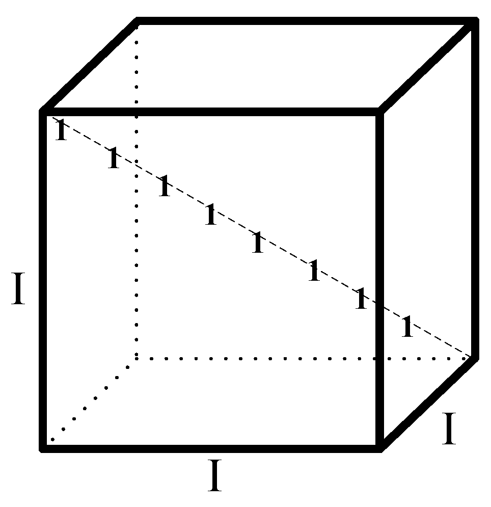
. If a tensor satisfies the conditions of both a cubical tensor and a diagonal tensor, the tensor is super-diagonal. On this basis, the tensor X is an identity tensor if and only if X is super-diagonal and [ X ] i , i , . . . , i = 1 for all i [ 1 , n ] . The 3rd-order identity tensor is shown in Figure 3.

4.1.4. n-Mode Product

The n-mode product of X R I 1 × I 2 × × I N with a matrix A R J × I n is denoted by X × n A , and the size of the result is I 1 × × I n 1 × J × I n + 1 × × I N . Elementswise, we have
[ X × n A ] i 1 , , i n 1 , j , i n + 1 , , i N = i n = 1 I n [ X ] i 1 , i 2 , , i N [ A ] j , i n .

4.2. Tensor Decomposition

Tensor decomposition can realize dimensionality reduction to solve the problem of dimensionality disaster in various tensor calculations and to dig the implicit relations in tensors. Two typical decomposition schemes in tensor decomposition are the CP Decomposition (CPD) and the Tucker decomposition.

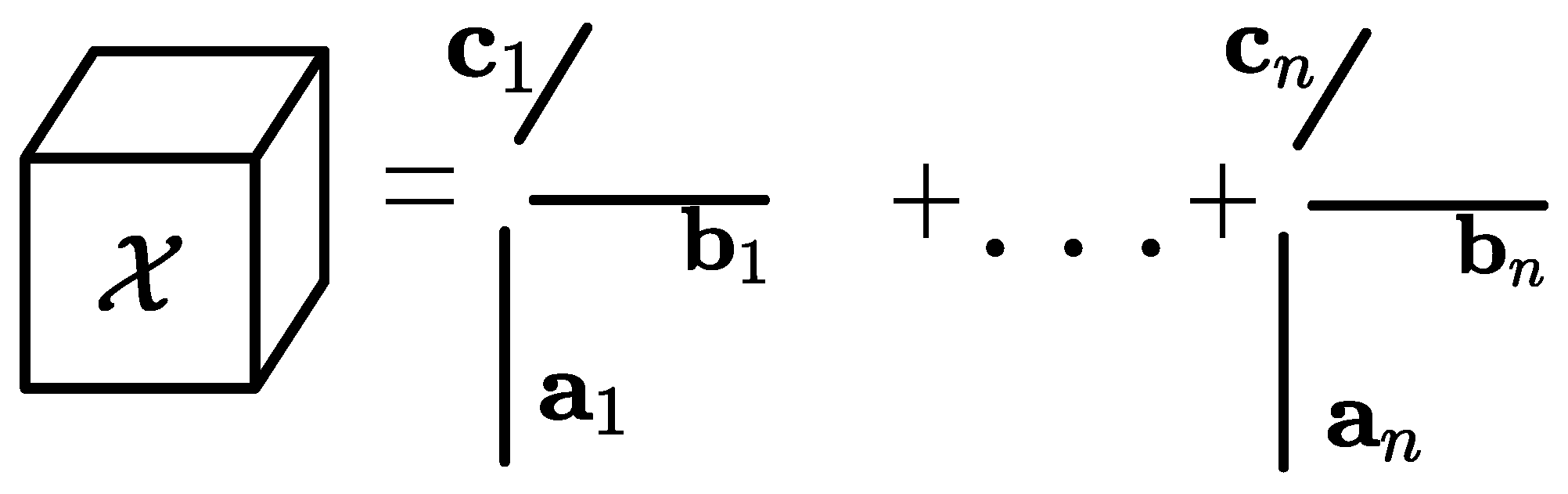
4.2.1. CP Decomposition

The CPD is to transform tensors into sums of rank-1 tensors. Set a third-order tensor X R I 1 × I 2 × I 3 , and the CPD of X can be written as
X = r = 1 R a r b r c r
where R is the tensor CP-rank, a r R I 1 , b r R I 2 , c r R I 3 . The process of CPD is illustrated in Figure 4.
The matrix composed of vectors that form rank-1 tensors is referred to as the factor matrix of CPD, such as A = a 1 , a 2 , a 3 a R , and the factor matrices B and C are defined the same. Based on the factor matrix, CPD can be more simply expressed as follows
X [ [ A , B , C ] ] r = 1 R a r b r c r .

4.2.2. Tucker Decomposition

Tucker decomposition can be expressed as
X G × 1 A × 2 B × 3 C = p = 1 P q = 1 Q r = 1 R [ G ] p , q , p a p b q c r = [ [ G ; A , B , C ] ]
where G R P × Q × R denotes the core tensor, and A R I × P , B R J × Q , C R K × R are three-factor matrices from three dimensions, as shown in Figure 5.
The scalar form is expressed as
[ X ] i , j , k p = 1 P q = 1 Q r = 1 R G p , q , r [ A ] i , p [ B ] j , q [ C ] k , r , i = 1 , 2 , , I ; j = 1 , 2 , , J ; k = 1 , 2 , , K .
When the core tensor G is a super-diagonal tensor, Tucker decomposition degenerates into CPD.

4.3. Tensor Completion

Considering the actual emergencies such as sensor failure, there is often some data loss in the data matrix, named missing values. Completion is to fulfill these missing values completely, and completion in the tensor is called tensor completion. The central issue in completion revolves around uncovering the association between missing values and observed values.
In order to introduce tensor completion, we take a classic tensor completion algorithm for the third-order tensors as an example, which is called high-accuracy low-rank tensor completion (HaLrTC), where the algorithm associates missing values with observed values through low rank based on the data sparsity hypothesis [35]. Given a sparse tensor X of size n 1 × n 2 × n 3 , the index set of the observed values is set to { Ω : ( i , j , k ) Ω } . Let the index tensor S with the same size of X satisfy
[ S ] i , j , k = 1 , ( i , j , k ) Ω 0 , ( i , j , k ) Ω .
The objective function of tensor completion is formulated as follows
min X ^ , A 1 , A 2 , A 3 A 1 ( 1 ) * + A 2 ( 2 ) * + A 3 ( 3 ) *
where X ^ denotes the estimation of the original tensor X , the size of tensors A 1 , A 2 , A 3 are n 1 × n 2 × n 3 , the matrix A 1 ( 1 ) with the size of n 1 × ( n 2 n 3 ) represents the mode-1 unfolding of tensor A 1 under mode-1 unfolding, and the meaning of matrix A 2 ( 2 ) and the matrix A 3 ( 3 ) is uniform as the former. In the objective function, the symbol · * is the norm for trace, which is the sum of the matrix singular values.
The optimization model is subject to two constraints, as illustrated in Equation (11). The initial constraint ensures equality between the elements of estimated tensor X ^ and original tensor X within Ω . The secondary constraint sets the intermediate variables A 1 , A 2 , and A 3 equal to the estimated tensors, serving as an optimization termination condition. The constraints are formulated as follows
S X ^ = S X X ^ = A q , q = 1 , 2 , 3
where the notation * represents the dot product, which means that the same index elements are directly multiplied.
The HaLrTC algorithm [35] is indicated in the Algorithm 1, in which fold q { } is the inverse process of tensor unfolding, that is, folding the matrix into the tensor in the order of unfolding.
Algorithm 1 HaLrTC algorithm
1:
Input index tensor S , adaptively changing ρ , residual threshold γ and maximum iteration number K.
2:
Initialize estimated tensor X ^ that [ X ^ ] i , j , k = [ X ] i , j , k , ( i , j , k ) Ω 0 , ( i , j , k ) Ω and the iteration number k = 0 .
3:
set zero transitional tensor T 1 , T 2 , T 3 R n 1 × n 2 × n 3 .
4:
Update A q : A q = fold q D α ̲ q ρ X ^ ( q ) + 1 ρ T q ( q ) , q = 1 , 2 , 3 , where D α q ρ ( X ) = U Σ α q ρ V T .
5:
Update X ^ : X ^ = ( 1 S ) 1 3 q = 1 3 A q 1 ρ T q + S * X .
6:
Update T q : T q = T q + ρ X ^ A q , q = 1 , 2 , 3 .
7:
If q = 1 3 A q X ^ γ , stop and output estimated tensor X ^ .
8:
If k < K , k = k + 1 , return to step 4. If not, stop and output estimated tensor X ^ .
9:
End.

4.4. Algorithm for Data Fusion

Data fusion, as a means of data processing, aims to transform two multi-dimensional heterogeneous mapping data matrices into a unified fusion matrix by tensor computing. Compared with the traditional data fusion scheme of direct splicing, the new data fusion scheme completely retains the original data information without matrix clipping. In the following meta-learning algorithm, the data information of the smart grid and power communication network can be obtained simultaneously by using the fusion data matrix.
The data of the smart grid and power communication network in Figure 1 can be mapped into the smart grid data matrix S R I S × J S and the power communication network data matrix C R I C × J C . Here, we assume that I S > J S and I C > J C . Then, the work to be completed is to combine these two data matrices into a fusion matrix while preserving the validity and structural relationship of the two data, that is, the fusion matrix can lossless restore two original data matrices after DF is complete. To complete the above work and achieve f ( : , : ) in (1), the algorithm is designed as follows.
After completing DF, the size of the fused data matrix D is I D × I D . In order to obtain a larger compression ratio, the columns of the matrix are completed to m a x ( J S , J C ) during the second step of the algorithm. However, this change will cause the fused matrix to lack a block of size ( I D m a x ( J S , J C ) ) × 2 I D / 3 . Without changing the fusion matrix arrangement, there is no difference between the two schemes in actual storage.
The third step reverses the Tucker decomposition. The identity matrix is used in the third-order direction to ensure the sparsity of the fusion tensor D without changing the value so as to facilitate the subsequent tensor completion operation, which is based on the sparsity of tensors. As mentioned in the Tucker decomposition above, Tucker decomposition degenerates to CP decomposition when the core tensor is hyper-diagonal. The core tensor D i n i in the algorithm is an identity tensor that satisfies the condition, and the resulting fusion tensor D can be reduced to the original matrices S and C by CP decomposition. Due to the uniqueness of CP decomposition, it is provable that the whole fusion algorithm is reversible. The specific algorithm is shown in Algorithm 2.
Algorithm 2 Data fusion algorithm based on tensor computing
1:
Input the smart grid data matrix S R I S × J S and the communication network data matrix C R I S × J S , adaptively changing ρ , fit index γ and maximum iteration number K.
2:
Initialize identity tensor D i n i R [ 3 , I D ] , where I D = m a x ( I S , I C ) , set the number of iterations k = 0 , and fulfill S and C with zero row vectors and zero column vectors to get S ^ R I D × I D and C ^ R I D × I D .
3:
Compute D = D i n i × 1 ( S ^ ) T × 2 ( C ^ ) T × 3 I , where I R I D × I D is a identity matrix.
4:
Use Algorithm 1 to generate D ^ .
5:
Set CP-rank R = I D / 3 , A 1 R I D × R , A 2 R I D × R , and A 3 R I D × R .
6:
Compute three sets of equations in sequence
V 1 = ( A 2 ) T A 2 ( A 3 ) T A 3 , A 1 = D ^ ( 1 ) ( A 3 A 2 ) V 1 ;
V 2 = ( A 1 ) T A 1 ( A 3 ) T A 3 , A 2 = D ^ ( 2 ) ( A 3 A 1 ) V 2 ;
V 3 = ( A 1 ) T A 1 ( A 2 ) T A 2 , A 3 = D ^ ( 3 ) ( A 2 A 1 ) V 3 .
7:
Compute D ^ = [ [ A 1 , A 2 , A 3 ] ] and f i t = 1 ( D ^ D ^ / ( D ^ .
8:
If f i t > γ , stop and output fused data matrix D = [ A 1 A 2 A 3 ] .
9:
If k < K , k = k + 1 , return to step 6. If not, stop and output fused data matrix D = [ A 1 A 2 A 3 ] .
10:
End.

5. Fault Diagnosis Based on Meta Learning

5.1. Meta Learning

Meta-learning introduces a range of concepts, including support set, query set, and N-way K-shot problems. The dataset of meta-learning can be divided into meta-training sets and meta-testing sets which, respectively, contain support sets and query sets used to support the training and testing of tasks.
When assessing the effectiveness of meta-learning models, the results of N-way K-shot problems are commonly used. Here, N signifies the number of classes, while K denotes the number of samples per class. Assuming there are N t r a i n classes in the meta-training set, with each class containing K t r a i n samples, and N t e s t classes in the meta-testing set, with each class containing K t e s t samples. N typically refers to the number of categories taken from the support set in the meta-testing set, while K represents the number of samples per class, where N < N t e s t and K < K t e s t . To maintain consistency between the meta-training and meta-testing stages, the model is trained on the meta-training set with the same number of categories and samples.
The Model-Agnostic Meta-Learning (MAML) algorithm is an outstanding algorithm in the field of meta-learning [36], continually optimizing the model’s generalization ability on new tasks by guiding the initialization parameters of the base learners. MAML is versatile, working well with various neural networks and different types of loss functions. It is similar to a learn skill that trains the initialization parameters of the model to achieve rapid convergence with limited sample data.
We assume that the MAML algorithm is applied to an image classification task. It is usually handled by the CNN model, so we use this model as the base-learner M b a s e to process image classification problems. Then MAML learns the parameters in the model training process as meta-knowledge and adjusts the initialization parameters on the new image classification task. Finally, we obtain the model M f i n e t u n e that is adapted to the new task.
The base-learner M b a s e can be represented as a function f θ with parameter θ . When the learner fits the new task T i , the parameters become θ . Based on the training samples in task T i , the base-learner M b a s e performs one or several gradient update iterations to update parameter θ . Assuming that one gradient update is required [36]
θ i = θ α θ L T i f θ
where α is the hyperparameter learning rate and L T i f θ is the loss function. The model parameter θ is updated by training the test samples from T i to optimize the performance of f θ i . Its objective function is
min θ T i p ( T ) L T i f θ i = T i p ( T ) L T i f θ α θ L T i f θ
The MAML aims to update the model parameters to produce the most efficient behavior. The model parameters θ are updated as
θ θ β θ T i p ( T ) L T i f θ i
where β represents the meta-update step size.
In practical applications, MAML demonstrates strong scalability across different datasets, but it also has some limitations. There needs to be a certain degree of similarity between the training and testing datasets; otherwise, it may lead to a decrease in generalization performance. Additionally, the multiple gradient updates performed in each iteration can result in longer training times and substantial computational resource consumption. Despite these limitations, MAML remains a highly effective meta-learning approach, particularly in terms of sample efficiency and generalization capabilities.

5.2. Fault Diagnosis in Power Communication Network and Smart Grid

5.2.1. Power Communication Network

When malfunctions occur within the power communication network, a substantial number of alarms are generated. These alarm notifications provide detailed information, including alarm device, alarm type, alarm level, alarm cause, and more. The alarm data primarily comprise three distinct categories: communication alarms, device-related alarms, and security alarms. Moreover, the alarm source and alarm name designate the unique identifier for the originating alarm and the nomenclature of the associated network element. These attributes constitute pivotal criteria for activities such as fault localization and fault classification.
To prepare the alarm information for subsequent utilization in feature vector extraction and training neural networks, a preprocessing stage is imperative. Initially, from the original alarm information database, relevant alarm information fields that exhibit substantial relevance to FD are meticulously selected. Furthermore, any redundant fields present within the original alarm database are systematically eliminated. Following this, standardization procedures are applied to ensure uniformity and consistency. Subsequently, the processed alarm dataset is subjected to a temporal and spatial synchronization procedure, employing a time window mechanism. Distinct alarms exert varying influence upon the ultimate determination of faults, signifying that these alarms possess disparate weights. These weights are utilized to establish a hierarchical order of priority, with higher weights signifying augmented precedence. Each distinct type of alarm is then subjected to a Boolean encoding process.
To depict the intricate topological interconnections existing between various sites within the power communication network, a graph theoretical approach involving an adjacency matrix is employed. Let G represent a graph encompassing m vertices (corresponding to sites), N ( G ) = n 1 , n 2 , . . . , n m represents the set of vertices within G, and E ( G ) signifies the set of edges. The adjacency matrix for G is denoted as A ( G ) = ( a i j ) m × m
a i j = 1 v i v j E ( G ) 0 v i v j E ( G ) i , j = 1 , 2 , , m .
When a malfunction occurs, the alarm transaction encodings of each site form a matrix T ( G ) = d i a g ( t 11 , t 22 , . . . , t m m ) , where t i i represents the alarm transaction encoding of the site n i . The mathematical expression for the fault state encoding matrix F ( G ) is
F ( G ) = A ( G ) T ( G ) .
After encoding the fault state matrix F ( G ) , the matrix is transformed into grayscale images and annotated with corresponding root cause fault labels. Finally, the fault state images from all instances of faults are compiled to form the training dataset. In the context of FD for the power communication network, the objective involves achieving fault localization and fault classification. As a result, for each fault state matrix, the corresponding root cause fault label is two-dimensional. This necessitates defining and encoding fault type labels and fault site labels.
Taking the power communication network of some cities in Shandong Province of China as an example, which is shown in Figure 6, there are a total of 30 network element sites. We select 12 sites among them and define fault site labels. The set of defined fault site labels is S 1 , S 2 , . . . , S 12 . As shown in Table 1, the simulated fault types in this study encompass five categories, and the set of defined fault type labels is F 1 , F 2 , F 3 , F 4 , F 5 . Train separately on the fault site label set and fault type label set to ultimately achieve the goal of fault localization and fault classification.

5.2.2. Smart Grid

We build a small current grounding fault simulation model within the Matlab Simulink module, utilizing the fault module to define various types of circuit faults, including single line-to-ground faults, double line faults, double line-to-ground faults and three-phase faults, comprising a total of 10 fault types. In which, single line-to-ground faults include Line A to Ground (AG), Line B to Ground (BG) and Line C to Ground (CG). Double line faults include Lines A and B (AB), Line B and C (BC) and Line A and C (AC). Double line-to-ground faults include Line A, B and Ground (ABG), Lines B, C and Ground(BCG), and Line A, C and Ground(ACG). Three phase faults include Lines A, B, C (ABC).
When the faults occur, fluctuations are observed in the voltage and current at both ends of the line. Thus, different fault types can be distinguished by observing changes in the magnitude and nature of these electrical parameters. We collect three-phase currents and voltages at both ends of the faulty line, denoted as V a , V b , V c , I a , I b , I c , and configure various system parameters to generate a dataset through batch simulations. The parameters for the fault samples are defined in Table 2.
The sampler is configured with a frequency of 1 kHz, a sampling time of 0.3 s, a fault initiation time of 0.1 s, and a fault clearing time of 0.15 s. Within a single sampling period, each sample contains 1800 data points. We extract 50 data points each from the six electrical parameters before and after the fault occurrence. The acquired data are then subjected to grayscale transformation according to Equation (18), resulting in the formation of grayscale images
x = x ( i ) min ( x ( i ) ) max ( x ( i ) ) min ( x ( i ) ) × 255
where x ( i ) represents the sequentially acquired electrical parameters, and x denotes the data after grayscale transformation. By altering parameters such as frequency and voltage, we obtain distinct fault grayscale images corresponding to different fault occurrences. These images collectively constitute the training dataset. The fault labels (AG, AB, etc.) are encoded, and the classification can be achieved using a meta-learning model.

6. Simulation Results and Theoretical Analysis

6.1. Evaluation Metrics and Model Parameters

The experimental setup includes a PC with Windows 10 operating system, an Intel(R) Xeon(R) Platinum 8255C CPU @ 2.50 GHz, two RTX 3080 (10 GB) GPUs, a development environment with Python 3.9.16, and a learning framework with PyTorch 1.11.0. For a 5-way 1-shot task, it requires GPU resources of at least 3 GB.
The experiment evaluates the performance of the model using accuracy ( A c c ), which is calculated as the ratio of correctly predicted samples to the total number of samples, as depicted in the following formula,
A c c = T P + T N T P + T N + F P + F N
where T P signifies true positive samples predicted by the model, T N signifies true negative samples predicted by the model, F P signifies false positive samples predicted as positive by the model, and F N signifies false negative samples predicted by the model.
Before conducting the experiment, it is essential to fine-tune the parameters of the model. While keeping other parameters constant, optimization is performed on the number of epochs, learning rate, and the minimum batch size. An epoch represents the process of training all training samples once. The model tends to stabilize after 30 epochs, so the number of epochs is set to 35. Fine-tuning the accuracy from 0.001 to 0.1 reveals that its impact on accuracy is minimal; thus, a learning rate of 0.001, which yields the optimal model performance, is selected. Additionally, adjusting the minimum batch size produces the results shown in Figure 7. The trends of both curves show an initial increase followed by a decrease, with both reaching their peak when the minimum batch size is set to 64. At this point, the model performs optimally, and thus, this parameter is chosen for subsequent experiments.

6.2. Performance of MAML Algorithm

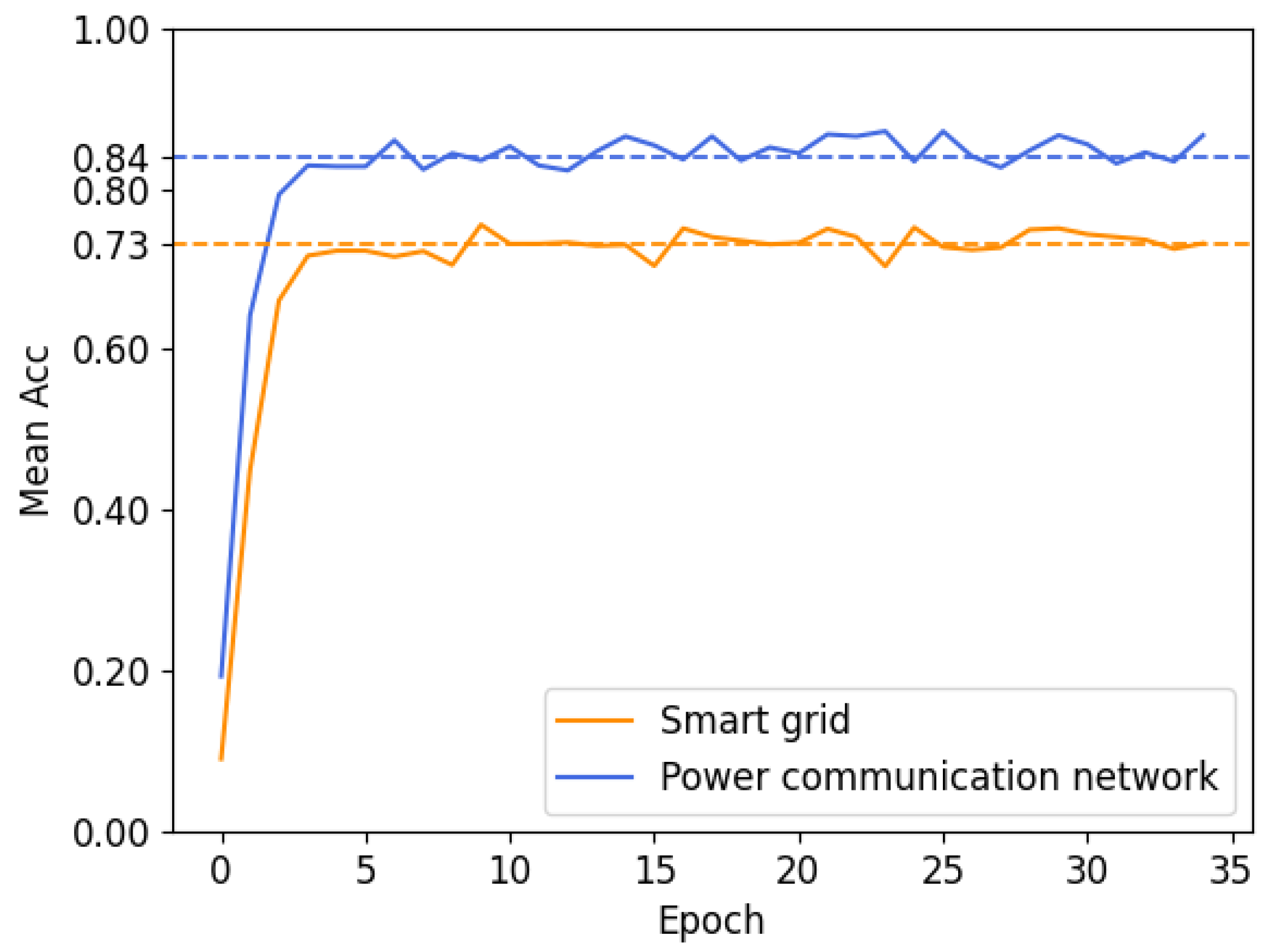
In this section, the performance of meta-learning is evaluated by comparing it with CNN. The results of model training are depicted in Figure 8. As shown in Figure 8, the blue line represents the power communication network, and the yellow line represents smart grid.
As the number of epochs increases, the model quickly converges, with the diagnosis accuracy reaching its peak as early as the fourth iteration. Due to differences in the number of fault types in the smart grid and the power communication network, the difficulty of fault diagnosis varies. As a result, the diagnosis accuracy for the power communication network is higher, fluctuating around 84%. In contrast, the diagnosis accuracy for the smart grid converges to 73%.
The performance of the MAML algorithm was assessed through a comparative analysis with a CNN model that was not equipped with MAML. The training results are depicted in Figure 9. It is clear that both smart grid and power communication networks experienced varying degrees of reduced diagnosis accuracy. The diagnosis accuracy of the smart grid decreased from the original 73% to 68%, and that of the power communication network dropped from the initial 84% to 66%.
In the simulation experiments for the smart grid, we sampled electrical quantities at different fault occurrences, processed them into grayscale samples, and modified system parameters such as frequencies and voltages to simulate the source and target domains. The dataset for the power communication network includes fault state matrices containing topological relationships and fault information. The disparities in topological relationships between the source and target domains necessitate the model to possess superior transferability. As a result, in the comparison between CNN and MAML, the diagnosis accuracy improvement for the power communication network was more pronounced than that of the smart grid.

6.3. Contribution of Data Fusion

The data processed by the DF model is a form of multi-modal heterogeneous data, comprising 10 fault types for the smart grid and five fault types for the power communication network. If converted into one-dimensional labels, the number of fault categories would increase to 50, which could adversely affect the model’s classification performance. Therefore, we chose to independently train networks for these two label categories. This approach allows for a more comprehensive utilization of the dataset and yields superior classification results. However, it is worth noting that training the same dataset twice requires more time.
After processing the feature-layer data with the DF model, we trained the fused data, which is based on Algorithm 2, and obtained model accuracy results based on various DF strategies. As shown in Figure 10 and Figure 11, both fusion approaches have improved diagnosis accuracy, but the extent of improvement varies. For the smart grid, using the CP decomposition scheme resulted in an increase of approximately 3% in accuracy, while the DF tensor scheme led to an improvement of around 6%. In the case of the power communication network, the CP decomposition approach raised accuracy by about 3%, while the DF tensor approach boosted it by approximately 8%. This demonstrates that, whether for the smart grid or the power communication network, the DF tensor scheme is superior.
Fused multi-modal data provide the model with additional information for decision-making, consequently enhancing diagnosis accuracy. CP decomposition addresses redundancy issues in the input space by reducing dimensions but can result in information loss. In contrast, the DF tensor retains all the original data’s information and exhibits superior diagnosis accuracy.

7. Conclusions

This paper explores DF and FD in smart grid and power communication networks based on tensor computing and meta-learning. For heterogeneous and multi-dimensional big data from two networks, after using matrix mapping, a tensor has been made use of operating the big data matrices and the tensor computing including tensor decomposition and tensor completion has been utilized to fuse those big data and generate the fused matrix. For the fused matrix, the meta-learning method has been used to train the two-network fused data fault detection scheme to sense the network fault state, under the case of insufficient training samples. Furthermore, the MAML algorithm has been proposed to address the FD problems, thereby tackling the challenge of limited and hard-to-obtain fault samples. The fault diagnosis accuracy of the MAML algorithm reaches 73% and 84% on the smart grid and power communication network, respectively, surpassing the accuracy of the CNN model. Additionally, among the two tensor fusion schemes, the DF tensor scheme exhibits superior optimization of the meta-learning model performance compared to the CP decomposition strategy. This paper offers practical guidance for managing big data in smart grids and power communication networks through DF and FD techniques.

Author Contributions

Conceptualization, M.S. and B.Q.; methodology, Q.Y. and M.S.; software, Q.Y. and L.L.; validation, T.G., Y.J. and Y.Z.; formal analysis, L.L.; investigation, T.G. and B.Q.; resources, A.T and Y.Z.; data curation, A.T.; writing—original draft preparation, Q.Y., M.S. and B.Q.; writing—review and editing, Y.J. and W.Z.; supervision, W.Z.; project administration, W.Z. All authors have read and agreed to the published version of the manuscript.

Funding

This research was funded by the Science and Technology project of State Grid Corporation of China (Research on Dispatching Fusion Communication Oriented to Power Communication Network and Its Cooperative Control with Power Network Operation, 52060022001B).

Institutional Review Board Statement

Not applicable.

Informed Consent Statement

Not applicable.

Data Availability Statement

Data are contained within the article.

Conflicts of Interest

Authors Qiusheng Yu, Anqi Tian, Yingjie Jiang, Yan Zhang, and Li Li are employed by the company Information & Telecommunications Company, State Grid Shandong Electric Power Company. Author Ti Guan is employed by State Grid Shandong Electric Power Company. The remaining authors declare that the research was conducted in the absence of any commercial or financial relationships that could be construed as a potential conflict of interest.

References

  1. Li, Y.; Duan, N.; Liu, Z.; Hu, J.; He, Z. Impedance-Matching-Based Maximum Power Tracking for Magnetic Field Energy Harvesters Using Active Rectifiers. IEEE Trans. Ind. Electron. 2023, 70, 10730–10739. [Google Scholar] [CrossRef]
  2. Butt, O.M.; Zulqarnain, M.; Butt, T.M. Recent advancement in smart grid technology: Future prospects in the electrical power network. Ain Shams Eng. J. 2021, 12, 687–695. [Google Scholar] [CrossRef]
  3. Zhou, M.; Rui, L.; Qiu, X.; Xia, Z.; Li, B. Evaluation of the Node Importance in Power Grid Communication Network and Analysis of Node Risk. In Proceedings of the 2018 IEEE/IFIP Network Operations and Management Symposium (NOMS 2018), Taipei, Taiwan, 23–27 April 2018; pp. 1–5. [Google Scholar]
  4. Wu, G.; Li, B.; Niu, J.; Gao, D.; Zhang, R. Study on Service Demand Model of Backbone Communication Network in New Power System. In Proceedings of the 2023 International Conference on Smart Electrical Grid and Renewable Energy (SEGRE), Changsha, China, 16–19 June 2023; pp. 153–159. [Google Scholar]
  5. Zhu, J.; Lu, W. Research on Converged Communication of Power Line and Wireless in Electric Power Communication System. In Proceedings of the 2021 IEEE 5th Information Technology, Networking, Electronic and Automation Control Conference (ITNEC), Xi’an, China, 15–17 October 2021; pp. 627–631. [Google Scholar]
  6. Wang, M.; Qu, Z.; He, X.; Li, T.; Jin, X.; Gao, Z.; Zhou, Z.; Jiang, F.; Li, J. Real Time Fault Monitoring and Diagnosis Method for Power Grid Monitoring and Its Application. In Proceedings of the 2017 IEEE Conference on Energy Internet and Energy System Integration (EI2), Beijing, China, 26–28 November 2017; pp. 1–6. [Google Scholar]
  7. Khalid, H.M.; Qasaymeh, M.M.; Muyeen, S.M.; El Moursi, M.S.; Foley, A.M.; Tha’er, O.S.; Sanjeevikumar, P. WAMS Operations in Power Grids: A Track Fusion-Based Mixture Density Estimation-Driven Grid Resilient Approach Toward Cyberattacks. IEEE Syst. J. 2023, 17, 3950–3961. [Google Scholar] [CrossRef]
  8. Khalid, H.M.; Flitti, F.; Mahmoud, M.S.; Hamdan, M.M.; Muyeen, S.M.; Dong, Z.Y. Wide area monitoring system operations in modern power grids: A median regression function-based state estimation approach towards cyber attacks. Sustain. Energy Grids Netw. 2023, 34, 101009. [Google Scholar] [CrossRef]
  9. Mao, X.; Shen, J.; He, J.; Fan, C.; Lou, J.; You, Q. Research on Fault Diagnosis Model Based on the Fusion of Communication Network and Grid Data. In Proceedings of the 2022 4th International Conference on Frontiers Technology of Information and Computer (ICFTIC), Qingdao, China, 2–4 December 2022; pp. 498–501. [Google Scholar]
  10. Liang, R.; Liu, F.; Qu, J.; Zhang, Z. A Bayesian-based Self-Diagnosis Approach for Alarm Prognosis in Communication Networks. In Proceedings of the 2019 8th International Symposium on Next Generation Electronics (ISNE), Zhengzhou, China, 9–10 October 2019; pp. 1–3. [Google Scholar]
  11. Hall, D.L.; Llinas, J. An Introduction to Multisensor Data Fusion. Proc. IEEE 1997, 85, 6–23. [Google Scholar] [CrossRef]
  12. Meng, T.; Jing, X.; Yan, Z.; Pedrycz, W. A Survey on Machine Learning for Data Fusion. Inf. Fusion 2020, 57, 115–129. [Google Scholar] [CrossRef]
  13. Liu, H.; Chen, Y.; Cui, N.; Xu, D.; Li, J. An Effective Data Fusion Model for Detecting the Risk of Transmission Line in Smart Grid. IEEE Internet Things J. 2022, 9, 22256–22266. [Google Scholar] [CrossRef]
  14. Kolda, T.G.; Bader, B.W. Tensor Decompositions and Applications. SIAM Rev. 2009, 51, 455–500. [Google Scholar] [CrossRef]
  15. Roy, S.; Menapace, W.; Oei, S.; Luijten, B.; Fini, E.; Saltori, C.; Huijben, I.; Chennakeshava, N.; Mento, F.; Sentelli, A.; et al. Deep Learning for Classification and Localization of COVID-19 Markers in Point-of-Care Lung Ultrasound. IEEE Trans. Med. Imaging 2020, 39, 2676–2687. [Google Scholar] [CrossRef]
  16. Zhu, K.; Zhang, T. Deep Reinforcement Learning Based Mobile Robot Navigation: A review. Tsinghua Sci. Technol. 2021, 26, 674–691. [Google Scholar] [CrossRef]
  17. Mahmud, M.; Kaiser, M.S.; Hussain, A.; Vassanelli, S. Applications of Deep Learning and Reinforcement Learning to Biological Data. IEEE Trans. Neural Netw. Learn. Syst. 2018, 29, 2063–2079. [Google Scholar] [CrossRef] [PubMed]
  18. Inayat, U.; Zia, M.F.; Mahmood, S.; Khalid, H.M.; Benbouzid, M. Learning-Based Methods for Cyber Attacks Detection in IoT Systems: A Survey on Methods, Analysis, and Future Prospects. Electronics 2022, 11, 1502. [Google Scholar] [CrossRef]
  19. Hospedales, T.; Antoniou, A.; Micaelli, P.; Storkey, A. Meta-Learning in Neural Networks: A Survey. IEEE Trans. Pattern Anal. Mach. Intell. 2022, 44, 5149–5169. [Google Scholar] [CrossRef] [PubMed]
  20. So, C. Exploring Meta Learning: Parameterizing the Learning-to-Learn Process for Image Classification. In Proceedings of the 2021 International Conference on Artificial Intelligence in Information and Communication (ICAIIC), Jeju Island, Republic of Korea, 13–16 April 2021; pp. 199–202. [Google Scholar]
  21. Metz, L.; Maheswaranathan, N.; Cheung, B.; Sohl-Dickstein, J. Meta-Learning Update Rules for Unsupervised Representation Learning. In Proceedings of the International Conference on Learning Representations (ICLR 2019), New Orleans, LA, USA, 6–9 May 2019; pp. 1–27. [Google Scholar]
  22. Ravi, S.; Larochelle, H. Optimization as A Model for Few-Shot Learning. In Proceedings of the International Conference on Learning Representations (ICLR 2017), Toulon, France, 24–26 April 2017; pp. 1–11. [Google Scholar]
  23. Lai, N.; Kan, M.; Han, C.; Song, X.; Shan, S. Learning to Learn Adaptive Classifier-Predictor for Few-Shot Learning. IEEE Trans. Neural Netw. Learn. Syst. 2020, 32, 3458–3470. [Google Scholar] [CrossRef] [PubMed]
  24. He, H.; Yan, J. Cyber-physical Attacks and Defences in the Smart Grid: A Survey. IET Cyber-Phys. Syst. Theory Appl. 2016, 1, 13–27. [Google Scholar] [CrossRef]
  25. Du, C.; Du, X.; Tong, C.; Li, Y.; Zhou, P. Stability Analysis for DFIG-Based Wind Farm Grid-Connected System under All Wind Speed Conditions. IEEE Trans. Ind. Appl. 2023, 59, 2430–2445. [Google Scholar] [CrossRef]
  26. Bessa, R.J.; Trindade, A.; Miranda, V. Spatial-Temporal Solar Power Forecasting for Smart Grids. IEEE Trans. Ind. Inform. 2015, 11, 232–241. [Google Scholar] [CrossRef]
  27. Qu, J.; Shi, W.; Luo, K.; Feng, C.; Mou, J. Day-Ahead Generation Scheduling Method for New Energy and Hydro Power System. In Proceedings of the 2018 International Conference on Power System Technology (POWERCON), Guangzhou, China, 6–8 November 2018; pp. 1899–1902. [Google Scholar]
  28. Fan, D.; Yi, Y.; Chen, S.; Song, L.; Li, J. Transmission Line Fault Type Identification based on Transfer Learning and Deep Learning. In Proceedings of the 2021 6th International Conference on Power and Renewable Energy (ICPRE), Shanghai, China, 17–20 September 2021; pp. 202–207. [Google Scholar]
  29. Isermann, R.; Ballé, P. Trends in the application of model-based fault detection and diagnosis of technical processes. Control Eng. Pract. 1996, 5, 709–719. [Google Scholar] [CrossRef]
  30. Vittori, A.D.; Cipollone, R.; Lizia, P.D.; Massari, M. Real-time space object tracklet extraction from telescope survey images with machine learning. Astrodynamics 2022, 6, 205–218. [Google Scholar] [CrossRef]
  31. Chen, H.; Jiang, B. A Review of Fault Detection and Diagnosis for the Traction System in High-Speed Trains. IEEE Trans. Intell. Transp. Syst. 2020, 21, 450–465. [Google Scholar] [CrossRef]
  32. Ran, G.; Chen, H.; Li, C.; Ma, G.; Jiang, B. A Hybrid Design of Fault Detection for Nonlinear Systems Based on Dynamic Optimization. IEEE Trans. Neural Netw. Learn. Syst. 2023, 34, 5244–5254. [Google Scholar] [CrossRef] [PubMed]
  33. Guo, Q.; Xin, S.; Wang, J.; Sun, H. Comprehensive Security Assessment for A Cyber Physical Energy System: A Lesson from Ukraine’s Blackout. Autom. Electr. Power Syst. 2016, 40, 145–147. [Google Scholar]
  34. Sun, X.; Zhan, W.H.; Li, Y. Fault Alarm Communication Scheduling Architecture and Method for Power System. In Proceedings of the 2022 IEEE 5th International Conference on Computer and Communication Engineering Technology, Beijing, China, 19–21 August 2022; pp. 271–274. [Google Scholar]
  35. Liu, J.; Musialski, P.; Wonka, P.; Ye, J. Tensor Completion for Estimating Missing Values in Visual Data. IEEE Trans. Pattern Anal. Mach. Intell. 2013, 35, 208–220. [Google Scholar] [CrossRef] [PubMed]
  36. Finn, C.; Abbeel, P.; Levine, S. Model-Agnostic Meta-Learning for Fast Adaptation of Deep Networks. In Proceedings of the International Conference on Machine Learning (ICLR 2017), Toulon, France, 24–26 April 2017; pp. 1126–1135. [Google Scholar]
Figure 1. Smart grid with power communication network.
Electronics 13 01655 g001
Figure 2. Framework of the system model.
Electronics 13 01655 g002
Figure 3. The 3rd-order identity tensor with size I × I × I .
Electronics 13 01655 g003
Figure 4. CPD for the 3rd-order tensor X .
Electronics 13 01655 g004
Figure 5. Tucker decomposition for the third-order tensor X .
Electronics 13 01655 g005
Figure 6. Power communication network topology in Shandong Province.
Electronics 13 01655 g006
Figure 7. Diagnosis accuracy for different batch sizes.
Electronics 13 01655 g007
Figure 8. Diagnosis accuracy of smart grid and power communication network based on MAML.
Electronics 13 01655 g008
Figure 9. Metatraining comparison results.
Electronics 13 01655 g009
Figure 10. Comparison of different DF approaches for smart grid.
Electronics 13 01655 g010
Figure 11. Comparison of different DF approaches for power communication network.
Electronics 13 01655 g011
Table 1. Fault types and labels.
Fault LabelFault Type
F1No fault
F2Ethernet interface not connected
F3Application board not installed
F4Board type mismatch
F5Device abnormal power loss
Table 2. Parameters of fault simulation model.
Parameter TypeParameter ValueParameter Quantity
Fault typeAG, BG, CG, AB, BC, AC,
ABG, BCG, ACG, ABC
10
Transient resistance/ Ω 1, 100, 200, 300, 400, 500,
600, 700, 800, 900
10
System frequency/Hz49, 50, 513
System voltage/kV400, 450, 5003
Disclaimer/Publisher’s Note: The statements, opinions and data contained in all publications are solely those of the individual author(s) and contributor(s) and not of MDPI and/or the editor(s). MDPI and/or the editor(s) disclaim responsibility for any injury to people or property resulting from any ideas, methods, instructions or products referred to in the content.

