1. Introduction
With the continuous development and progress of society, people have higher and higher requirements for power quality. Frequency stability is an important indicator to measure the power quality of power systems [
1,
2]. Automatic generation control (AGC) has received widespread attention from scholars as an important means to maintain system frequency stability, ensure system power balance, and improve power quality in modern power systems [
3]. Load frequency control [
4] (LFC) is usually regarded as the core part of AGC in the power system. It aims to ensure that the frequency of the power system and the exchange power of inter-regional tie lines are maintained near the rated value, thereby allowing the interconnected power system to operate safely and reliably.
In today’s society, the demand for fossil energy such as coal and oil is increasing year by year, leading to the continued deterioration of the global environment and the increasing depletion of fossil energy. In response to this problem, countries around the world have turned their attention to the development and utilization of new energy. On the one hand, new energy has the innate advantage of being green, low-carbon, and renewable; on the other hand, it also has certain disadvantages. With the large-scale integration of renewable energy sources such as wind and light into the power grid with randomness and uncertainty, frequency controllers designed for conventional power systems can no longer meet the control needs. Therefore, the interconnection of large-scale renewable energy power generation units is crucial to conduct LFC strategy research on power systems.
The emergence of the interconnected power system has made the distribution of energy in various regions more reasonable and the distribution of electricity more balanced, effectively solving a series of problems caused by uneven energy distribution in various regions and the tight power supply in some areas. Interconnected power systems have significant advantages in solving the problem of uneven energy and load distribution, making them an important trend in the development of modern power systems. However, there are inevitably some potential risks in interconnected power systems. On the one hand, as the scale of interconnected systems becomes larger and larger, the structure of the power system becomes more complex, which is not conducive to system state observation; on the other hand, due to the large amount of wind power, photovoltaic and other new energy sources have been integrated into the power grid, which has brought great challenges to the stability of the system frequency [
5]. Therefore, in order to make the interconnected power system more widely used, we urgently need to solve the problems of frequency stability of the interconnected power system and safe operation of large-scale power systems.
As the scale and complexity of modern power systems gradually increase, various advanced control algorithms have been studied to varying degrees in LFC, such as sliding mode control [
6,
7,
8], robust control [
9,
10], automatic adaptive control [
11,
12] and model-predictive control [
13,
14,
15], etc. However, although the advanced control methods mentioned above have improved the LFC performance of the power system, these methods are not suitable for application in engineering practice because of their complex structures and excessive information requirements. Therefore, in most practical projects, the classic PI controller with its simple structure and easy implementation is still used [
16]. However, considering the randomness and uncertainty of renewable energy sources, such as wind energy and solar energy, which have a series of impacts on the frequency control of interconnected power systems, this article will propose a simple and practical control strategy to meet the needs of existing power systems. The problem of correct frequency control is difficult.
In recent years, active disturbance rejection control [
17] (ADRC) has developed rapidly due to its strong immunity to disturbance and its independence from mathematical models of controlled objects. Its core idea is mainly through expanded state observation. The device estimates and compensates the system model and external disturbances in real time, thereby ensuring that the system has strong anti-disturbance capabilities [
18]. However, although ADRC can show good control performance in many fields, its parameter-tuning process is cumbersome and its structure is complex. Therefore, Dr. Gao Zhiqiang from Cleveland State University proposed a simple structure Linear Active Disturbance Rejection Control (LADRC) [
19,
20]. In addition to being beneficial to its parameter adjustment, the proposal of LADRC also greatly promotes the application of active disturbance rejection control theory in engineering practice. In view of this, this article will use LADRC to control the load frequency of interconnected power systems containing large-scale renewable energy in order to achieve better control effects.
For the parameter optimization problem of LADRC, this paper uses Particle Swarm Optimization (PSO). This algorithm is simple in concept, easy to program, and has fast convergence speed. However, it also inevitably has the problem of a premature algorithm, making it easy to settle for the local optimal solution. In view of this, this paper proposes an improved PSO algorithm based on Levy flight and chaotic mapping, aiming to improve its optimization effect.
This paper constructs a load frequency control model of a three-region interconnected power system containing renewable energy in MATLAB, uses LADRC to control the model, and uses the improved PSO algorithm to optimize its parameters. The simulation results show that the improved algorithm outperforms the original one. Compared with the original algorithm, the active disturbance rejection controller has better tracking performance and smaller deviation value, thus showing its good control performance.
2. Load Frequency Control
As a key component of AGC, LFC is mainly responsible for regulating the generation power of generators in response to changes in system frequency. Specifically, the core goal of load frequency control is to maintain the system frequency within the specified value range to ensure the stable operation of the power system. To achieve this, the LFC monitors the system frequency and automatically adjusts the output power of the generator based on its changes to bring the system frequency back to the normal range.
In an interconnected power system, area control error (ACE) can effectively reflect the imbalance between power generation and load supply and demand through the deviation of current load active power, generation active power and frequency. During the operation of the power system, because the active power load of the power system changes irregularly every moment, the generator set cannot respond in time with the change of the load, which will lead to the deviation of the system frequency and the exchange power of the liaison line. In order to make the deviation of the system frequency and the exchange power of the liaison line zero in the steady state, it is necessary to control and adjust the generator set according to the regional control deviation
ACE. In general, the area control deviation
ACE can be expressed by Equation (1):
where: Δ
Ptiei is the switch-line power deviation, Δ
fi is the system frequency deviation, and
Bi is the frequency deviation coefficient.
This paper studies a three-area interconnected power system including wind power and photovoltaic, and the mathematical models of each system will be introduced successively in the following sections.
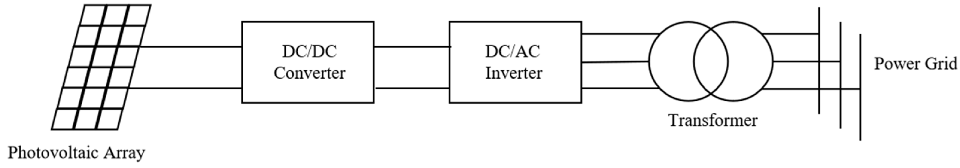
2.1. Model of Photovoltaic Power Generation System
Photovoltaic Generator (PVG) is a device that converts solar light energy directly into electrical energy, and its basic principle is the photoelectric effect. The structure of a photovoltaic grid-connected system mainly includes photovoltaic panel, maximum power point tracking (MPPT) controller, DC/DC converter and inverter. The realization process is that the sun shines on the photovoltaic panel, the photovoltaic cell in the panel absorbs the light energy, generates direct current, and then the direct current is boosted by the DC/DC converter as the DC power supply of the inverter, in this process, to achieve the maximum power point tracking of the photovoltaic cell, and then converted into alternating current by the inverter to the power grid. The grid-connected structure of photovoltaic power generation is shown in
Figure 1:
The DC/DC converter controls the power output of the PVG by adjusting the DC terminal voltage. In order to make the photovoltaic array still output at maximum power when the external light changes, it is necessary to change the output voltage of the photovoltaic array to make it work at the maximum power point; this control method, which involves changing the output voltage of the photovoltaic array to track the maximum power point, is called the maximum power point tracking control. This allows the control system of the DC/DC converter to operate below the MPPT value so that the PVG has sufficient power reserves to enable it to participate in frequency regulation. The transfer function of the photovoltaic power generation system involved in frequency regulation can be expressed as follows [
21,
22]:
where: Δ
Ppv is the change in the generated electric power; Δ
Pref is the system control signal.
The literature [
23] proposes a PVG model suitable for LFC research, which regards PVG as a “negative” load and its transfer function can be expressed as follows:
where: Δ
Ppv is the change in the generated electric power; Δ
G is for changes in the sun’s illumination;
Kpv = 1;
Tpv = 1.8 s.
2.2. Wind Power System Model
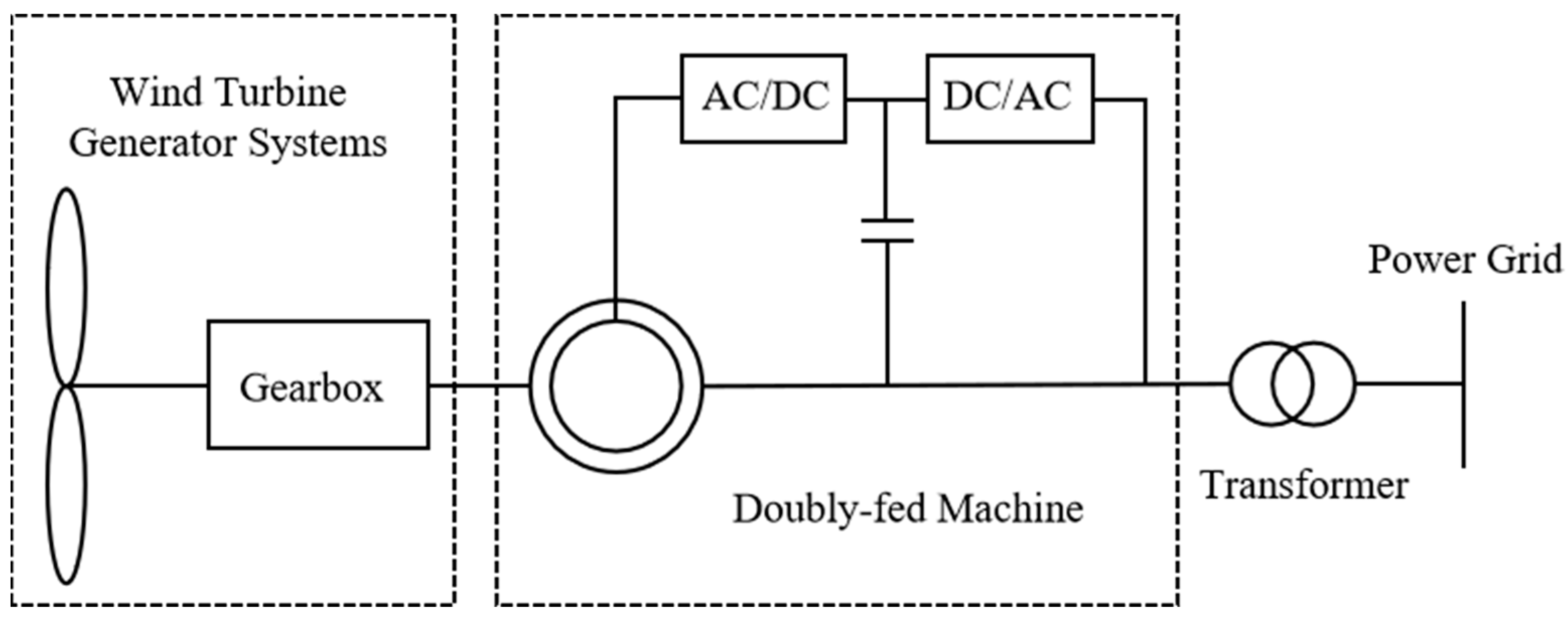
Wind Turbine Generator (WTG) is the core component of the wind power system, mainly by capturing the wind to drive the turbine blade rotation, so as to prompt the mechanical transmission system to convert the rotational kinetic energy into electricity. The wind power generation system can be divided into two categories according to the grid-connected mode: constant speed constant frequency wind generator and variable speed constant frequency wind generator, of which the variable speed constant frequency wind generator usually uses permanent magnet synchronous motor or a Doubly-Fed Induction Generator (DFIG). Since DFIG allows wind turbines to operate at a wide range of wind speeds, thereby enabling them to capture wind energy more efficiently, and can maintain high power generation efficiency over a wide range of wind speeds, reducing the loss of energy capture, this paper will introduce DFIG into the load frequency control model of interconnected power systems. The basic structure of DFIG is shown as follows (
Figure 2):
Similar to PVG, it is assumed that WTG operates below its maximum power point, reserving a certain uplink and downlink frequency modulation capacity. When the system needs frequency modulation support, WTG can participate in the adjustment of the system frequency by increasing or reducing the generation power. A linear WTG model suitable for LFC research was introduced in the literature [
24], which consists of two transfer functions:
where:
Gwp(
s) is the first transfer function;
Gwl(
s) is the second transfer function; parameter
KPC is called the blade characteristic and has a constant value of 0.8.
Gwp(
s) changes in output power are simulated by changing the pitch angle of the blade using a variable pitch actuator, which can be expressed as follows:
where:
.
Gwl(
s) is a first-order lag used to match the phase/gain characteristics of the model to the experimental data, which can be expressed as follows:
where:
KP2 is a constant.
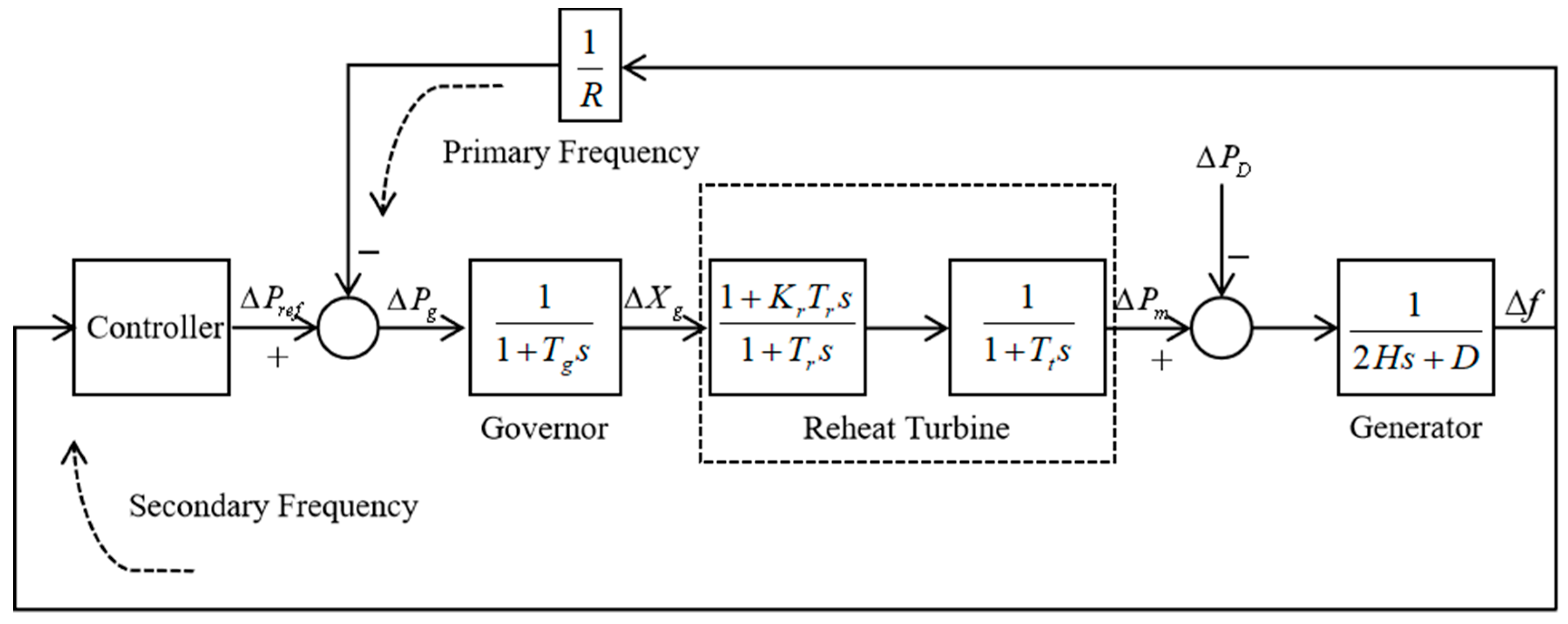
2.3. Thermal Power System Model
A thermal power system is usually composed of a governor, steam turbine and generator; its specific composition is shown in
Figure 3.
In
Figure 3, Δ
Pref is the system control signal;
Tg is the time constant of the governor; Δ
Xg is the change of valve position;
Tr is the reheat time constant;
Kr is the ratio of the power generated by steam in the high-pressure cylinder segment to the total power of the turbine;
Tt is the turbine time constant; Δ
Pm is the prime mover output mechanical power deviation;
R is the adjustment coefficient; h is the system frequency deviation.
The transfer function of a turbine governor can usually be expressed as follows:
where: Δ
Xg is the change of valve position;
Tg is the time constant of the governor.
The working principle of the steam turbine is to use high-temperature and high-pressure water vapor to drive the rotor to rotate, so as to achieve the conversion of thermal energy to mechanical energy. Because the steam volume phenomenon exists in the operation of the steam turbine, the change of the valve cannot immediately affect the mechanical power, so a first-order inertia link is often used to express the regulation process of the steam volume to the steam turbine.
For reheating the steam turbine, the reheat stage filling delay should also be considered, and its transfer function can be expressed as follows:
where:
Tt is the time constant of the steam boiling process;
Tr is the reheat time constant, generally about 10 s;
Kr is the ratio of the power generated by the steam in the high-pressure cylinder segment to the total power of the turbine, generally 0.2 to 0.3 times the total power of the turbine.
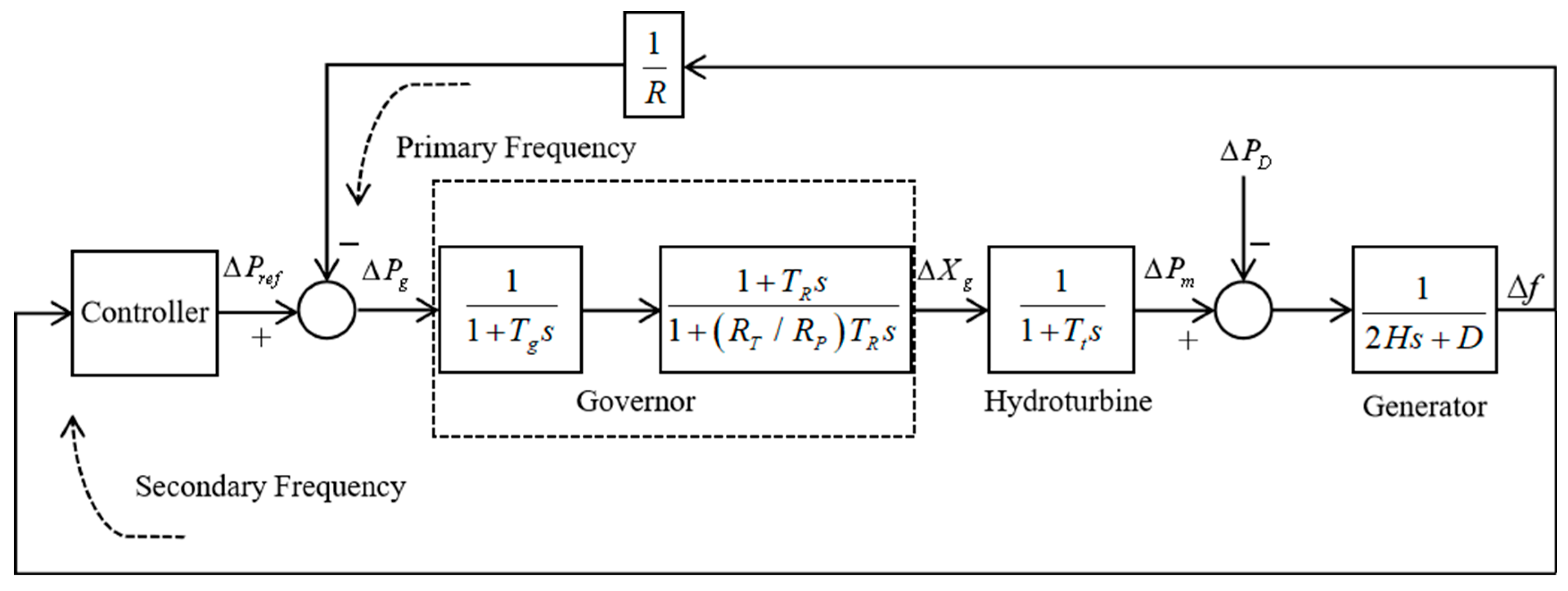
2.4. Hydropower System Model
A hydropower system is usually composed of a governor, turbine and generator; the specific composition is shown in
Figure 4.
In
Figure 4, Δ
Pref is the system control signal;
Tg is the time constant of the governor; Δ
Xg is the change of valve position;
TR is reset time constant;
RT is the transient decline rate;
RP is the permanent decline rate;
Tt is the time constant of the turbine; Δ
Pm is the prime mover output mechanical power deviation;
R is the adjustment coefficient; Δ
f is the system frequency deviation.
Due to the strong lag of the hydraulic turbine, the traditional hydraulic turbine governor usually adopts the governor, including the transient slope compensation, so its transfer function model can be expressed as follows:
where:
TR is reset time constant;
RT is the transient decline rate;
RP is the permanent decline rate.
Different from the steam turbine, the water turbine also needs to consider the water hammer effect, and its transfer function can be expressed as follows:
where:
Tw is the water hammer time constant.
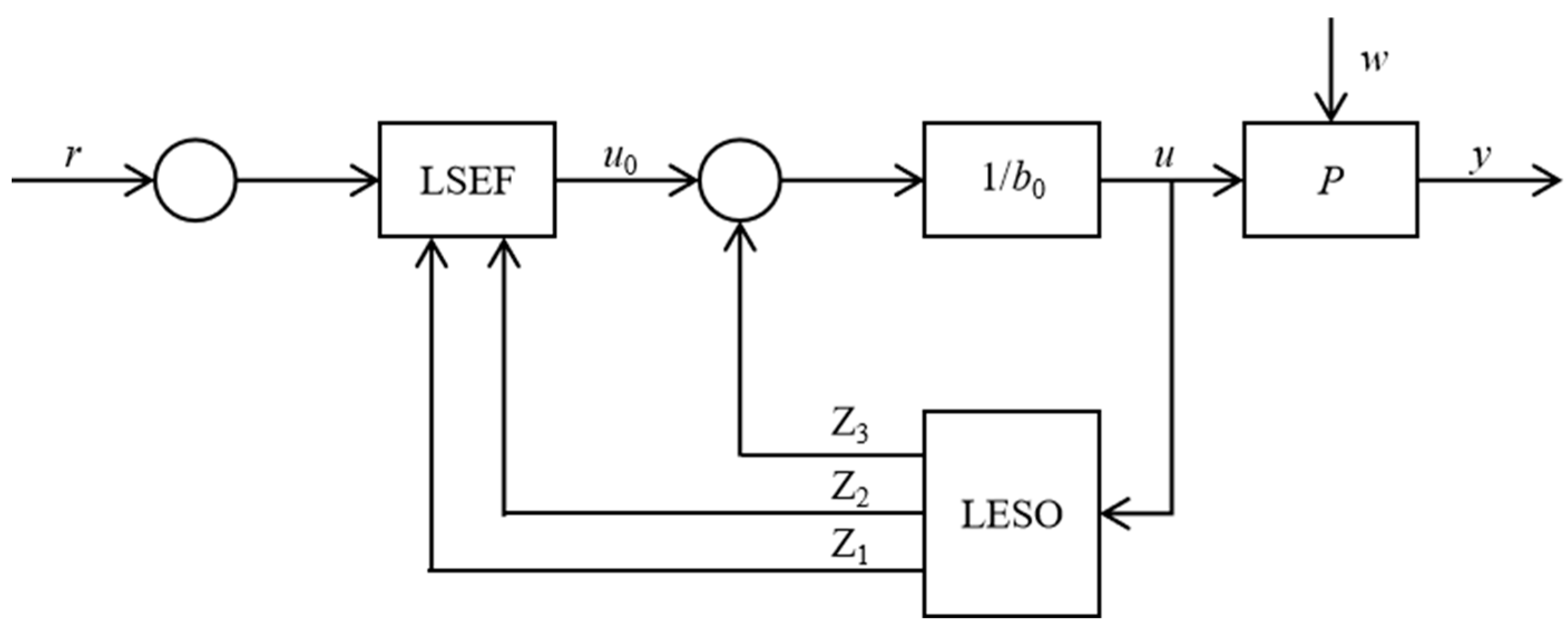
3. Linear Active Disturbance Rejection Control
The essence of active disturbance rejection control is that when the disturbance of the system has a great impact on the output, it can actively extract relevant disturbance information from the input or output signal of the controlled object and eliminate it, thereby effectively reducing the impact on the controlled variable. While LADRC retains the original advantages of ADRC, it can also simplify the parameters that need to be tuned to only three, making it more advantageous in engineering practice. On the one hand, the use of nonlinear functions is reduced, and the control structure is made simpler by linearizing each link, which is beneficial to the parameter setting of the controller and the performance analysis of the system; on the other hand, it has stronger stability and robustness when dealing with system disturbances, can better estimate system disturbances, and maintain stable control effects when the system is disturbed. The basic idea of LADRC is to treat the generalized disturbance of the system as an expanded state and use a linear expanded state observer to achieve state estimation. The advantage of this method is that it can estimate various disturbances of the control system in real time, and, through simplified design, it makes the process of tuning the state observer and controller easier.
Taking the second-order system as an example, the simplified basic structure of LADRC is shown in
Figure 5.
Assume that the mathematical model of the controlled object is as follows:
In Equation,
y,
u and
w are, respectively, the output, input and disturbance of the system, b contains part of known information
b0, and r is the set value, that is:
where:
f is the sum of unknown dynamics and external disturbances of the system.
Choose, as the state variable of the system, the following:
where:
z3 is the new state variable of the system expanded by total disturbance. Assuming
f is differentiable, Equation (11) can be expressed as follows:
where:
After the extended state, A designs a full-order state observer for the system:
where:
is the observer error feedback gain, which can be obtained by sorting out the following:
When
in Equation (16) is asymptotically stable,
, it indicates that the system has estimated the disturbance, and the following control law can be designed to reduce the influence of the disturbance on the system:
By substituting Equation (17) into Equation (12), we achieve the following:
When the observer is properly designed,
, then Equation (18) becomes as follows:
Use the PD control combination to control the system:
where:
is a set of controller parameters that need to be designed.
The controller parameter-tuning problem is essentially a multi-objective optimization problem, which needs to consider the characteristics of load interference suppression, measurement noise attenuation, setpoint tracking and robustness at the same time. In process control, on the premise of ensuring the stability of the system, load interference suppression is the main problem to be considered.
For LADRC, the controller parameters can be tuned by adjusting the ESO and feedback control bandwidth, so, similar to PID controllers, LADRC can be considered a fixed-structure controller with multiple tuning parameters.
According to the above principle analysis process, the whole LADRC controller only needs to set the following two sets of parameters: the error feedback gain L0 of the extended state observer and the control parameter K of the PD control combination.
For Equation (16), the poles of its characteristic Equation are placed on the observer bandwidth:
In this case, the gain matrix of the extended state observer is as follows:
For the PD control combination, when the observer can accurately estimate the system disturbance, Equation (20) is substituted into Equation (15) to obtain the following:
Similarly, the poles of the characteristic equation of Equation (23) are placed at the controller bandwidth:
After the simplification of the above parameters, it can be seen that the parameters that LADRC needs to adjust are observer bandwidth, controller bandwidth and disturbance compensation gain.
4. Improved Particle Swarm Algorithm
4.1. Basic Principles of Particle Swarm Algorithm
The particle swarm algorithm is a swarm intelligence optimization algorithm proposed by American scholars James Kenendy and Russel Eberhart in 1995 through the analysis and research of bird foraging behavior. In this algorithm, a particle refers to each individual in the entire population, which can be represented by its position and speed in the population. Based on this, the basic principle of PSO can be expressed as that in a given multi-dimensional search space; each particle in the population learns based on its own experience to learn the optimal position combined with the optimal position unanimously recognized by other members of the entire population. It adjusts its position to determine its own flight speed and direction, thereby gradually optimizing group behavior. Assume that, in a multi-dimensional search space, group
X is composed of m particles. The position of each particle in the group represents a solution to the optimization problem. Select an appropriate fitness function as an evaluation criterion for its optimization. If the best position searched by each particle in the
KTH iteration is
Pid, combined with the best positions searched by all the other particles in the population, a best position is selected as the group’s best position
Pgd, then the
i+. The velocity and position formulas that need to be updated for a particle at the
k + 1 iteration can be expressed as follows:
In the Equation, k is the current number of iterations, w is the inertia weight, c1 and c2 are learning factors, r1 and r2 are two random numbers in the range of (0, 1) to ensure the diversity of the group, and is the particle swarm. The local optimal solution of a particle is the global optimal solution of the particle swarm; the position of the particle when iterating k times is the speed of the particle when iterating k times, where the position and speed of the particle will be limited to and respectively.
4.2. Improved Particle Swarm Algorithm
In view of the shortcomings of the PSO algorithm, such as fast early convergence and easy falling into local optimality, scholars from all over the world have proposed various improved PSO algorithms through continuous research. Through continuous practice and application, they have found that these methods can indeed greatly improve the optimization performance of the PSO algorithm. But these methods also have their unavoidable limitations. In view of this, this section proposes a particle swarm optimization algorithm based on Levy flight and chaotic mapping, aiming to solve the problem of fast early convergence and easy falling into local optimality. Research has found that the introduction of chaotic mapping can bring randomness to the PSO algorithm, allowing particles to jump out of the local optimal solution area, thereby preventing the particle swarm from falling into the local optimum. It can also increase the diversity of the particle swarm, allowing the particle swarm to expand its search space; the introduction of Levy flight can improve the search accuracy of the PSO algorithm through its random step characteristics and help particles jump out of the local optimal solution area.
4.2.1. Levy Flight
The PSO algorithm is an optimization algorithm that simulates the foraging behavior of a flock of birds. It finds the optimal solution through collaboration and information sharing between particles. There are many advantages to introducing Levy’s flight into the PSO algorithm. The unconventional jump of Levy’s flight can show higher efficiency when exploring complex search spaces, improve the performance of the algorithm, and is suitable for many applications in complex optimization problems, etc.
Considering that the Levy distribution is relatively complex, Mantegna algorithm simulation is usually used to obtain the Levy flight step size in practical applications:
In the equation,
and
v obey the normally distributed random numbers of the following Equation:
where:
where:
is a scalar;
is the gamma function;
is usually 1.5.
According to the characteristics of Levy’s flight, random step length and keeping its flight speed unchanged, the position update formula of the improved PSO algorithm can be expressed as follows:
where:
is the step factor;
s is a random step.
4.2.2. Tent Chaotic Mapping
Chaos is an extremely complex nonlinear theory in nature. Chaos theory believes that, in a chaotic system, when an extremely small change in the initial conditions occurs, after continuous development, it will bring unpredictable random effects to its future state. The core of chaos theory lies in its unpredictability and sensitivity to initial conditions. These characteristics allow chaotic mapping to generate pseudo-random sequences that have good uniformity and randomness in spatial distribution. By introducing chaotic variables to replace or adjust certain parameters in PSO (such as the position and velocity of particles), the coverage of the search space can be effectively increased, preventing the algorithm from prematurely converging to the local optimal solution, thereby improving the overall performance of the algorithm. Specifically, the advantages of introducing chaotic mapping are mainly reflected in the following aspects:
- (1)
Enhance global search capabilities: Improving the randomness and diversity of the algorithm will help the algorithm jump out of the local optimal solution and enhance global search capabilities.
- (2)
Improve the convergence speed: Through chaos search, you can converge to the global optimal solution or approximate optimal solution faster.
- (3)
Strong adaptability: Being able to adapt to various types of optimization problems, especially showing good performance when dealing with complex and multi-peak optimization problems.
There are many types of chaos mapping rules, and different chaos mappings also have different chaos intervals and sensitivities.
Table 1 lists several common chaos mapping formulas.
Precisely because each chaotic mapping has its own unique properties, different chaotic mappings will definitely bring about different optimization effects. Logistic mapping has been favored by many scholars because of its simplicity, easy implementation, and uniform distribution. However, compared with logistic mapping, Tent mapping also has its unique and excellent attributes, such as good correlation and uniform probability density distribution. Therefore, this article decided to use Tent mapping as the mapping rule to improve particle swarm initialization. This article will introduce the Tent chaos map to perform a chaotic search on the particle position variables, and then compare the fitness values before and after the search, so as to achieve the purpose of updating the particle position variables.
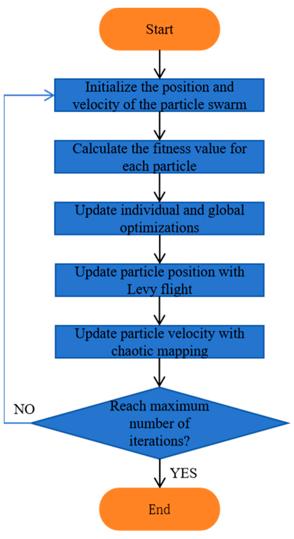
4.2.3. IPSO Algorithm Principle and Process
The particle swarm optimization algorithm based on Levy flight and Tent chaos mapping aims to find optimal solutions by simulating complex phenomena in nature. This algorithm introduces the fractal structure of Levy’s flight and the sensitivity of Tent chaos mapping, so that the particle swarm can better explore the solution space during the search process, avoid falling into the local optimal solution, and improve the search efficiency.
The flow chart of the particle swarm optimization algorithm based on Levy’s flight and Tent chaos mapping involves combining the long-step search characteristics of Levy’s flight with the ability to quickly traverse the initial solution space of Tent chaos mapping to enhance the global search of the PSO algorithm. The IPSO algorithm flow chart is shown in
Figure 6.
4.2.4. IPSO Algorithm Performance Test
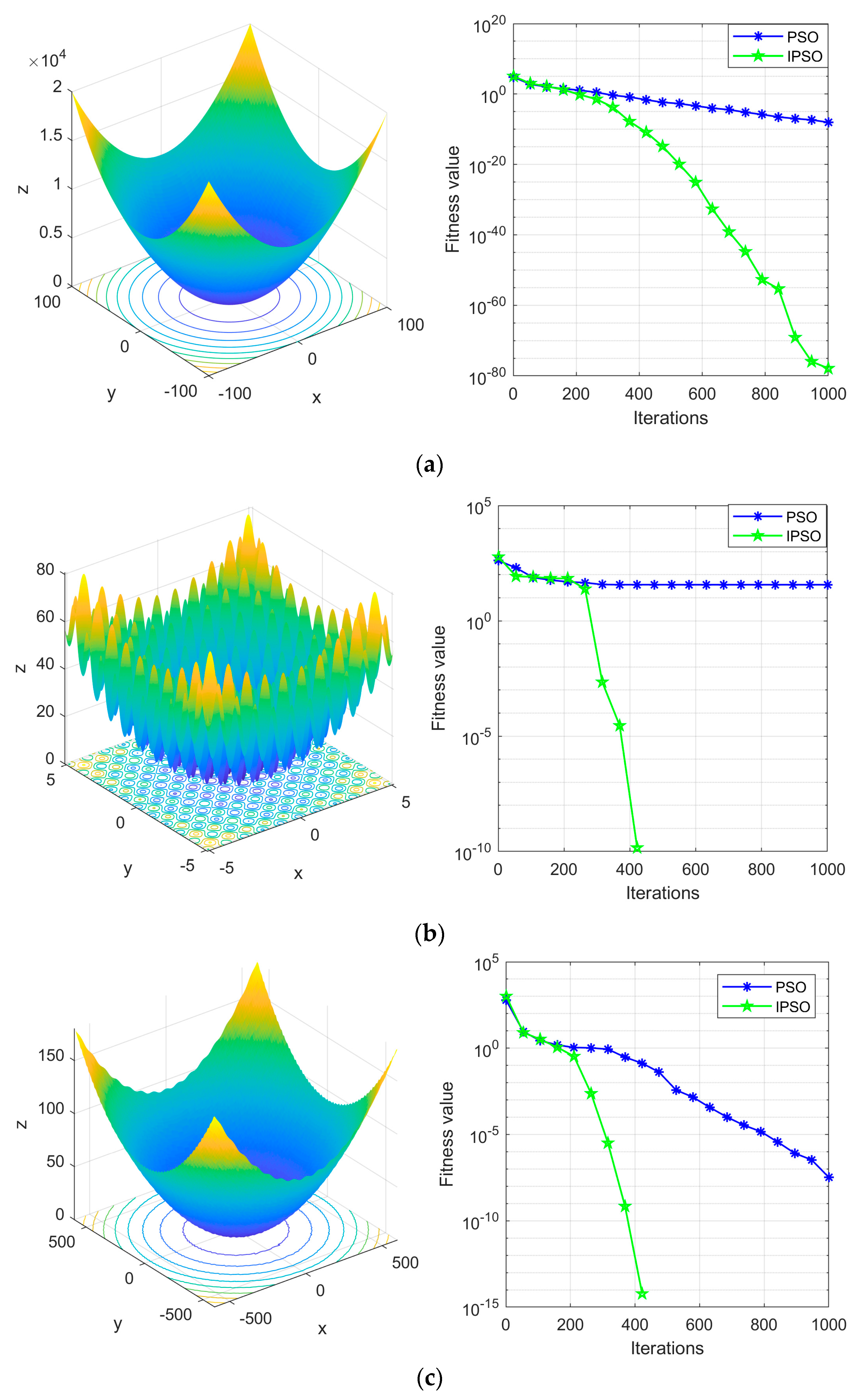
In order to verify the performance of the IPSO algorithm mentioned above, this paper conducts a comparative test of the IPSO and PSO algorithms. In the simulation experiment, some reference functions with different characteristics are selected for testing.
Table 2 lists the definition, value range, theoretical optimal value and dimension of the above test functions, respectively.
The test was carried out on the above three functions. The dimension of the test function was set to 30, the population number of the PSO algorithm and IPSO algorithm was set to 50, the learning factors c1 and c2 were both set to 1.2, the inertia weight of the PSO algorithm was 0.85, the inertia weight of the IPSO algorithm was 0.8, and the number of cycles was 1000.
In order to more clearly compare the convergence speed of the above two algorithms, the evolution process curves under the above three test functions are shown in
Figure 7. It can be clearly seen from
Figure 7 that the convergence effect of the IPSO algorithm is better than that of the PSO algorithm, and the convergence speed of the IPSO algorithm is also significantly improved compared with the PSO algorithm.
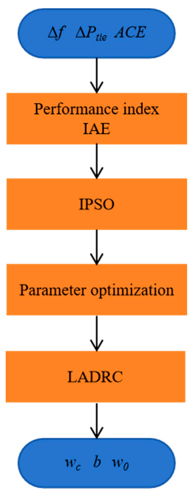
In this paper, the most commonly used criterion, Integral of Absolute Error (IAE), will be selected as the fitness function of the reaction controller performance. The specific expression of IAE is as follows:
IAE mainly reflects the total amount of difference between the output and the expected output during the system’s response to a given input or disturbance. A lower IAE value usually means better control performance. Comparing the LADRC optimized by the standard PSO and improved PSO algorithms,
Table 3 shows the performance indicators of frequency deviation, tie-line exchange power deviation and regional control deviation in each region.
It can be seen more intuitively from the table that there is a certain gap between the improved PSO-optimized LADRC and the PSO-optimized LADRC. Taking the IAE of ACE1 as an example, it can be seen that the IAE value of the standard PSO-optimized LADRC is more than 3 times greater than that of the improved PSO-optimized LADRC, thus confirming that the improved PSO-optimized LADRC has higher response speed and tracking accuracy. In view of this, in order to ultimately obtain better dynamic performance of the control system, this article will select appropriate parameters to optimize the objective function according to the IPSO algorithm in the LADRC control system, thereby obtaining appropriate LADRC parameters. The basic process is shown in
Figure 8.
5. Simulation Results and Discussions
A three-area interconnected power system model containing renewable energy was constructed by MATLAB/Simulink to verify the frequency modulation performance of the proposed method under the action of load disturbance.
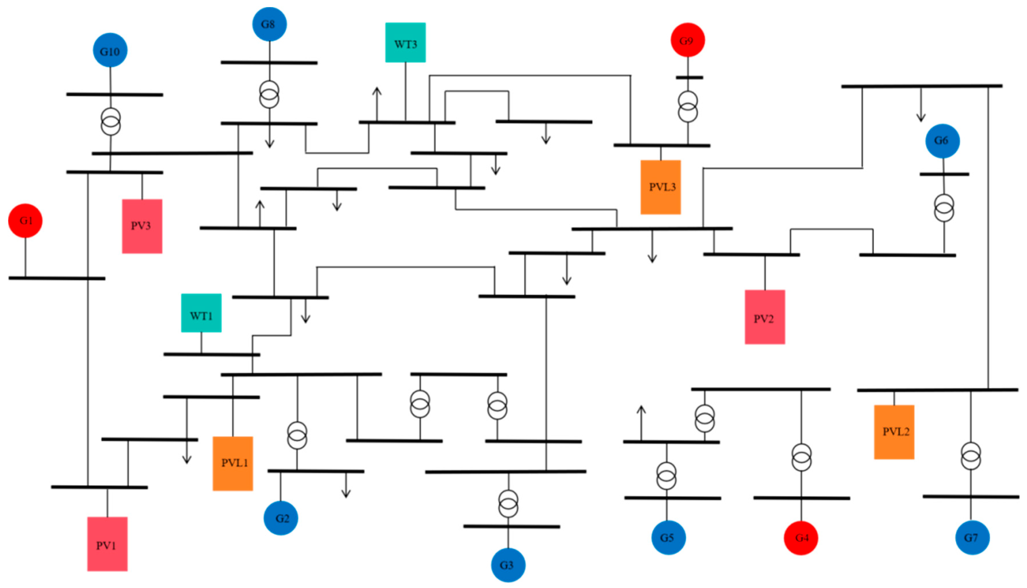
Figure 9 shows the model diagram of the three-region interconnected power system. Based on the classic IEEE-39 node system, this model artificially divides the system into three control areas, and adds PVG and WTG to some nodes of the system.
In area 1, G1 is a thermal generator, G2 and G3 are hydroelectric generators, PV1 and PVL1 are photovoltaic generators, and WT1 is a wind turbine; in area 2, G4 is a thermal generator, and G5, G6, and G7 are hydroelectric generators. PV2 and PVL2 are photovoltaic generators; in area 3, G8 is a thermal generator, G8 and G10 are hydroelectric generators, PV3 and PVL3 are photovoltaic generators, and WT3 is a wind turbine. In areas 1 and 3, PVG and WTG participate in secondary frequency adjustment at the same time. In area 2, only PVG participates in secondary frequency adjustment, and each control area has a PVG introduced in the form of “negative” load.
The participation factor reflects the relative sensitivity of each generator in responding to changes in system frequency. In order to ensure that the power system has sufficient spinning reserve, the selection of participation factors in each area should ensure that thermal generators can participate in secondary frequency regulation to the maximum extent. The participation factors of generators in each region are shown in
Table 4.
The torque coefficient of the connecting line in the interconnection area is shown in
Table 5.
The relevant parameters of the generator are shown in the following table (
Table 6,
Table 7 and
Table 8):
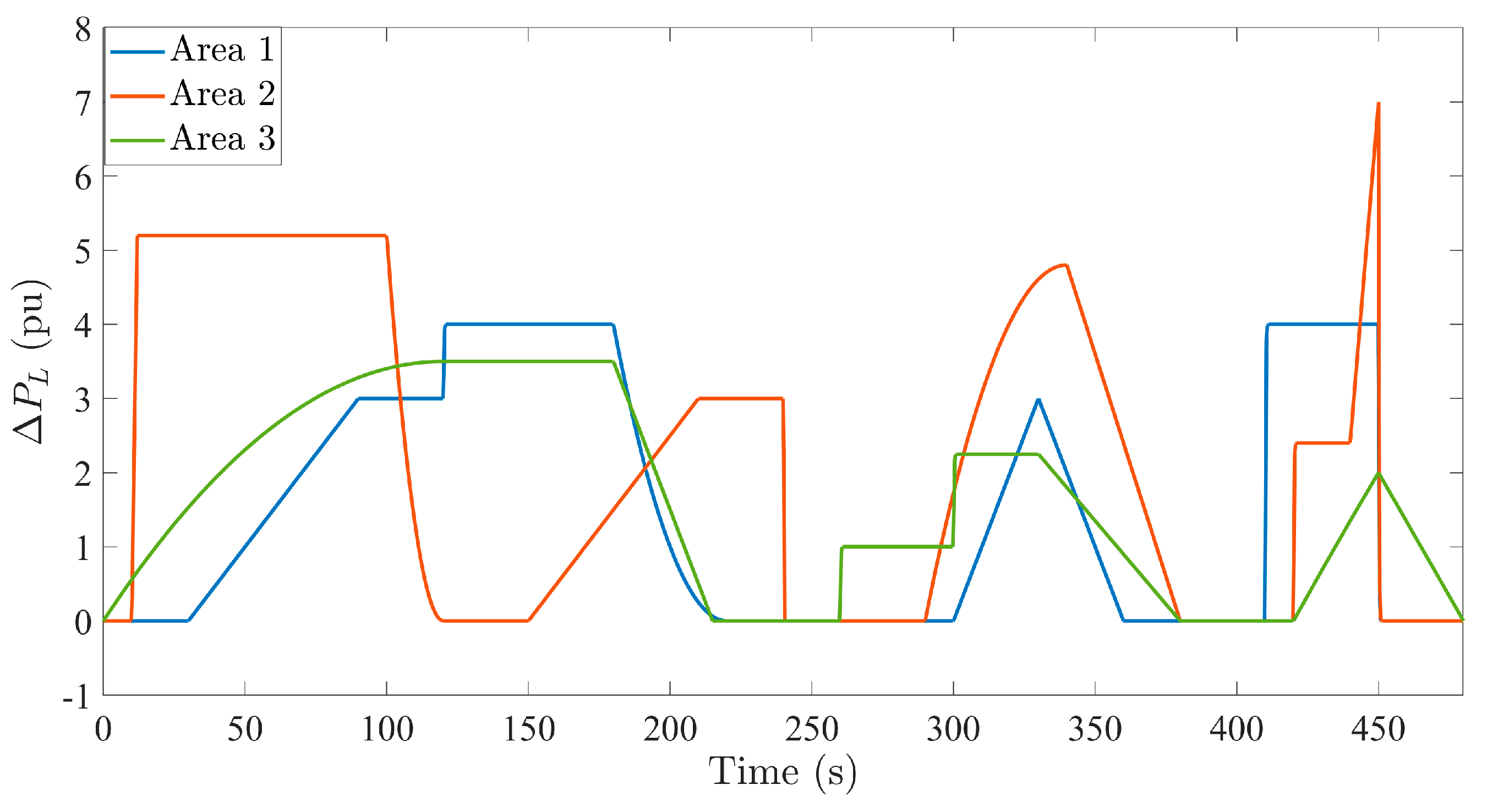
Load disturbance in each control area is shown in
Figure 10.
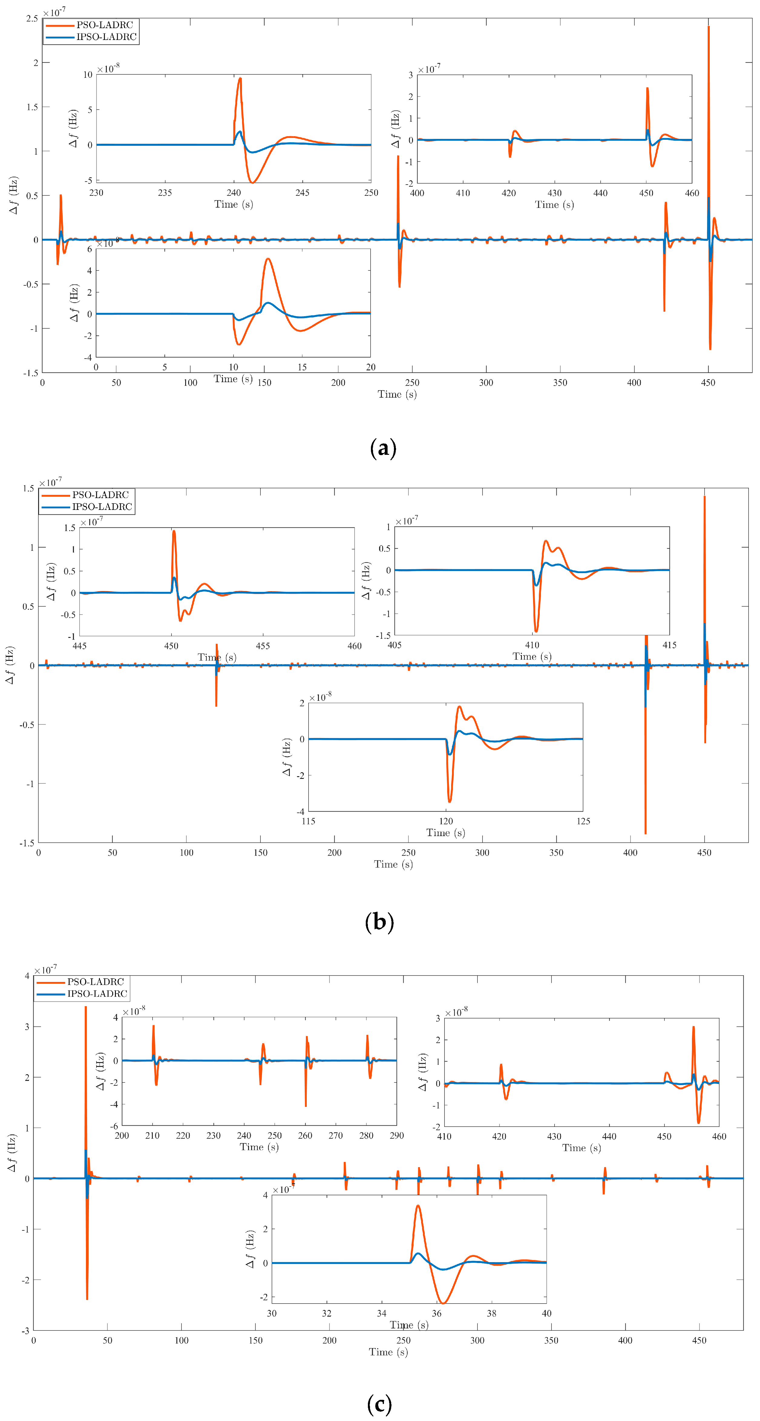
It can be clearly seen from
Figure 11 that the controller optimized by the algorithm obviously performs much better in dynamic performance indicators than the controller without algorithm optimization, and its frequency deviation is not even an order of magnitude; in addition, when the system has large load disturbances, it can be found that the controller optimized by the IPSO algorithm can better track the changes in load disturbance and have a smaller frequency deviation than the controller optimized by the PSO algorithm.
Specifically, it can be clearly seen from the partial enlargement of area 1 that the maximum frequency deviation of the system controlled by the LADRC controller optimized by the algorithm still occurs at 450 s. Among them, there is the maximum frequency deviation of the system controlled by the LADRC controller optimized by the PSO algorithm. The frequency deviation is 1.42 × 10⁻⁷, while the maximum frequency deviation of the system controlled by the LADRC controller optimized by the IPSO algorithm is only 0.38 × 10⁻⁷, a year-on-year decrease of 73.34%. In area 2, there is the LADRC control optimized by the PSO algorithm. The maximum frequency deviation of the system controlled by the controller is 2.38 × 10⁻⁷, while the maximum frequency deviation of the system controlled by the LADRC controller optimized by the IPSO algorithm is 0.47 × 10⁻⁷, a year-on-year decrease of 80.25%. Similarly, in area 3, the maximum frequency deviation of the system controlled by the LADRC controller optimized by the PSO algorithm is 3.43 × 10⁻⁷, while the maximum frequency deviation of the system controlled by the LADRC controller optimized by the IPSO algorithm is 0.51 × 10⁻⁷, a year-on-year decrease of 85.14%. It can be seen that the control strategy proposed in this article can effectively improve the frequency stability of the system.
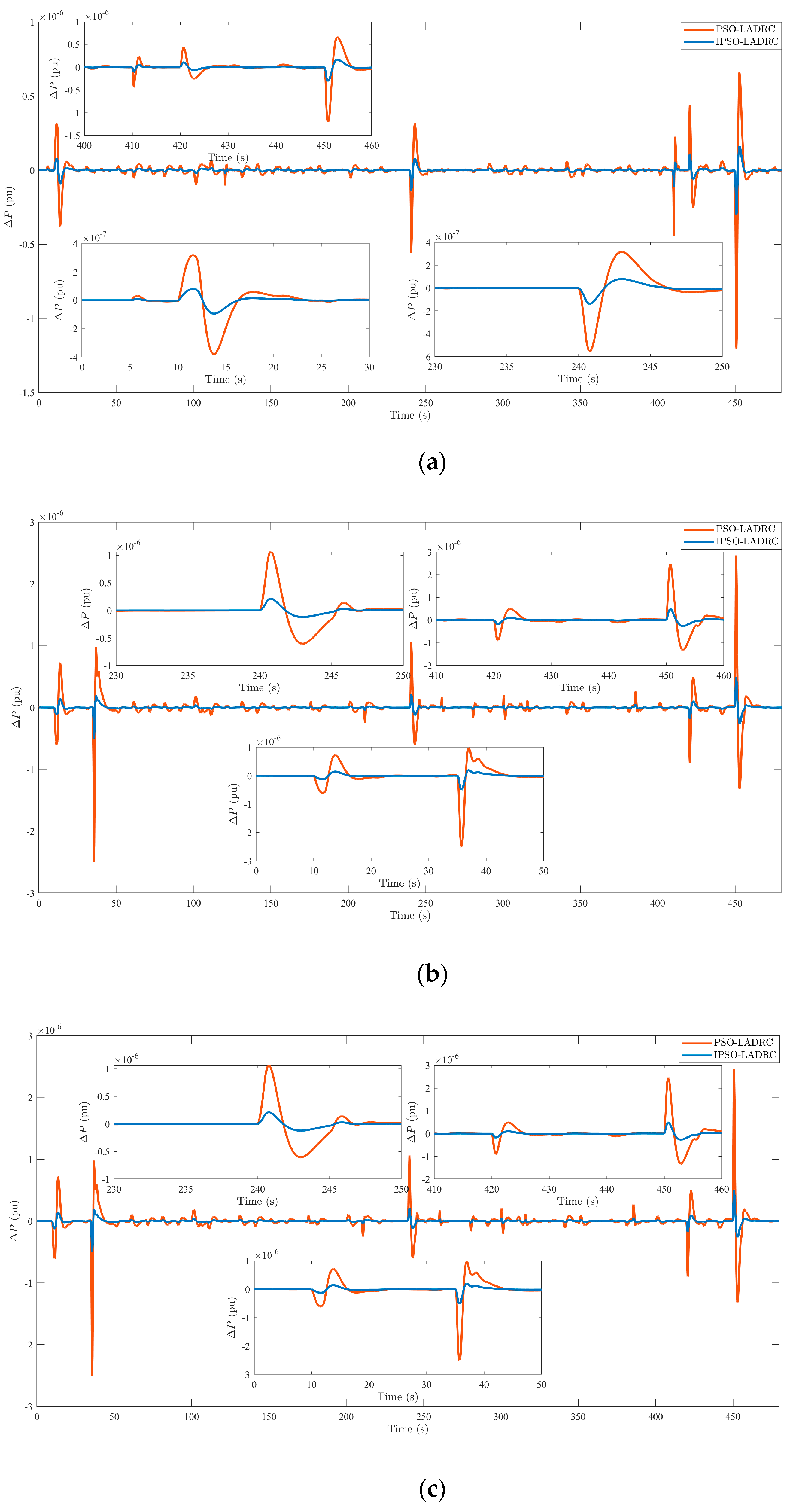
The exchange power deviation of the lines between regions is shown in
Figure 12.
It can be seen from
Figure 12 that, after algorithm optimization, there is still a certain tie line exchange power deviation in the system, but compared with the controller without algorithm optimization, it has obviously been greatly improved; on the other hand, it can still be seen that the controller optimized by the IPSO algorithm has a smaller tie line exchange power deviation than the system controlled by the controller optimized by the PSO algorithm.
Specifically, it can be clearly seen from the partial enlargement of
Figure 12a that the maximum inter-regional tie line exchange power deviation of the system controlled by the LADRC controller optimized by the PSO algorithm is −1.23 × 10
−6, and the maximum frequency deviation of the system controlled by the LADRC controller optimized by the IPSO algorithm is only −0.32 × 10
−6, a year-on-year decrease of 73.98%; in the maximum frequency deviation of the system controlled by the LADRC controller optimized by the PSO algorithm between area 2–3, the deviation is 2.37 × 10
−6, while the maximum frequency deviation of the system controlled by the LADRC controller optimized by the IPSO algorithm is 0.42 × 10
−7, a year-on-year decrease of 82.28%; similarly, between area 3–1 optimized by the PSO algorithm, the maximum frequency deviation of the system controlled by the LADRC controller is 4.0 × 10
−6, while the maximum frequency deviation of the system controlled by the LADRC controller optimized by the IPSO algorithm is 0.61 × 10
−6, a year-on-year decrease of 84.75%. It should be known that the controller optimized by the IPSO algorithm can significantly reduce the exchange power deviation of the tie line, which also proves its excellent control effect.
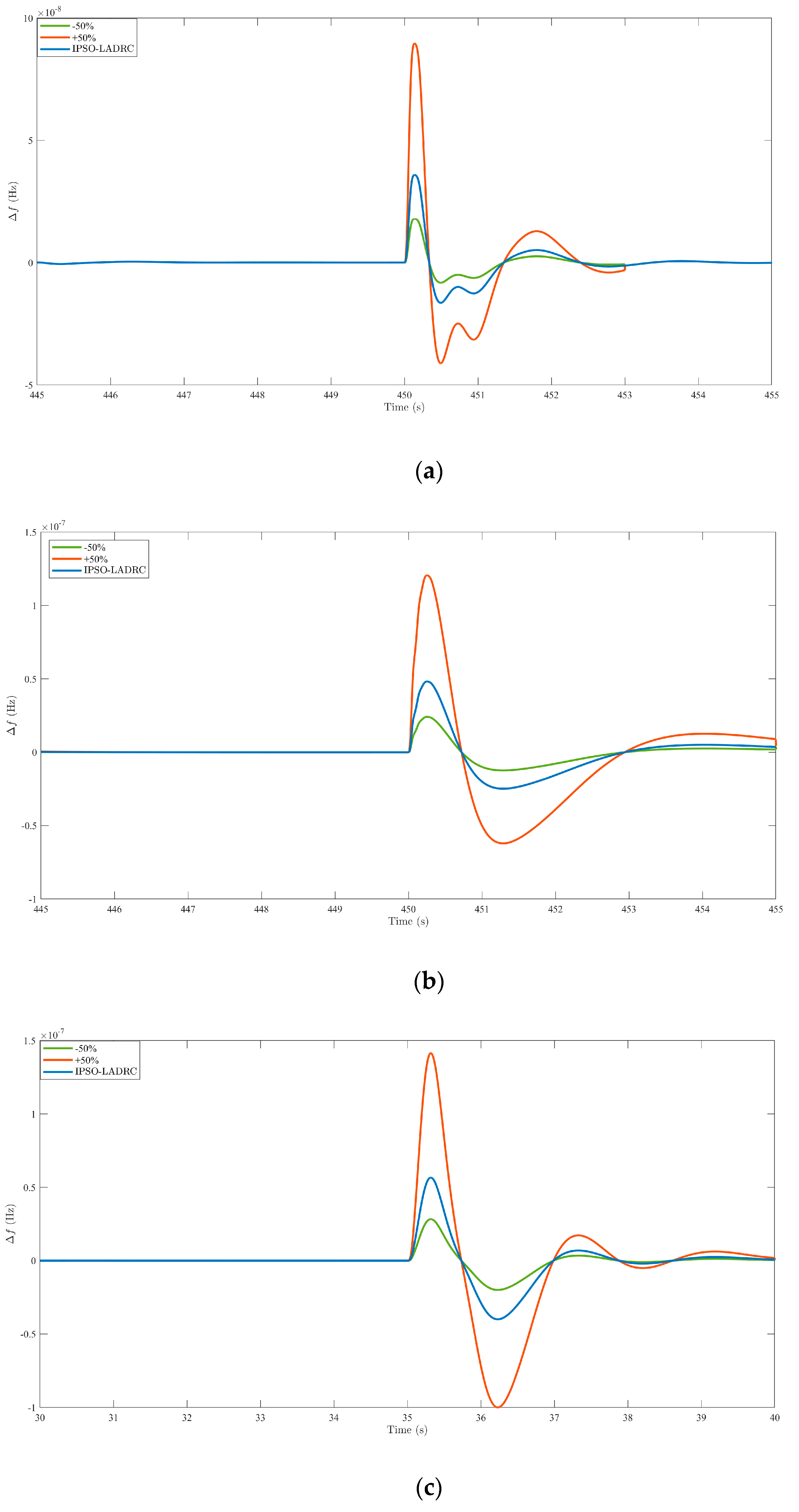
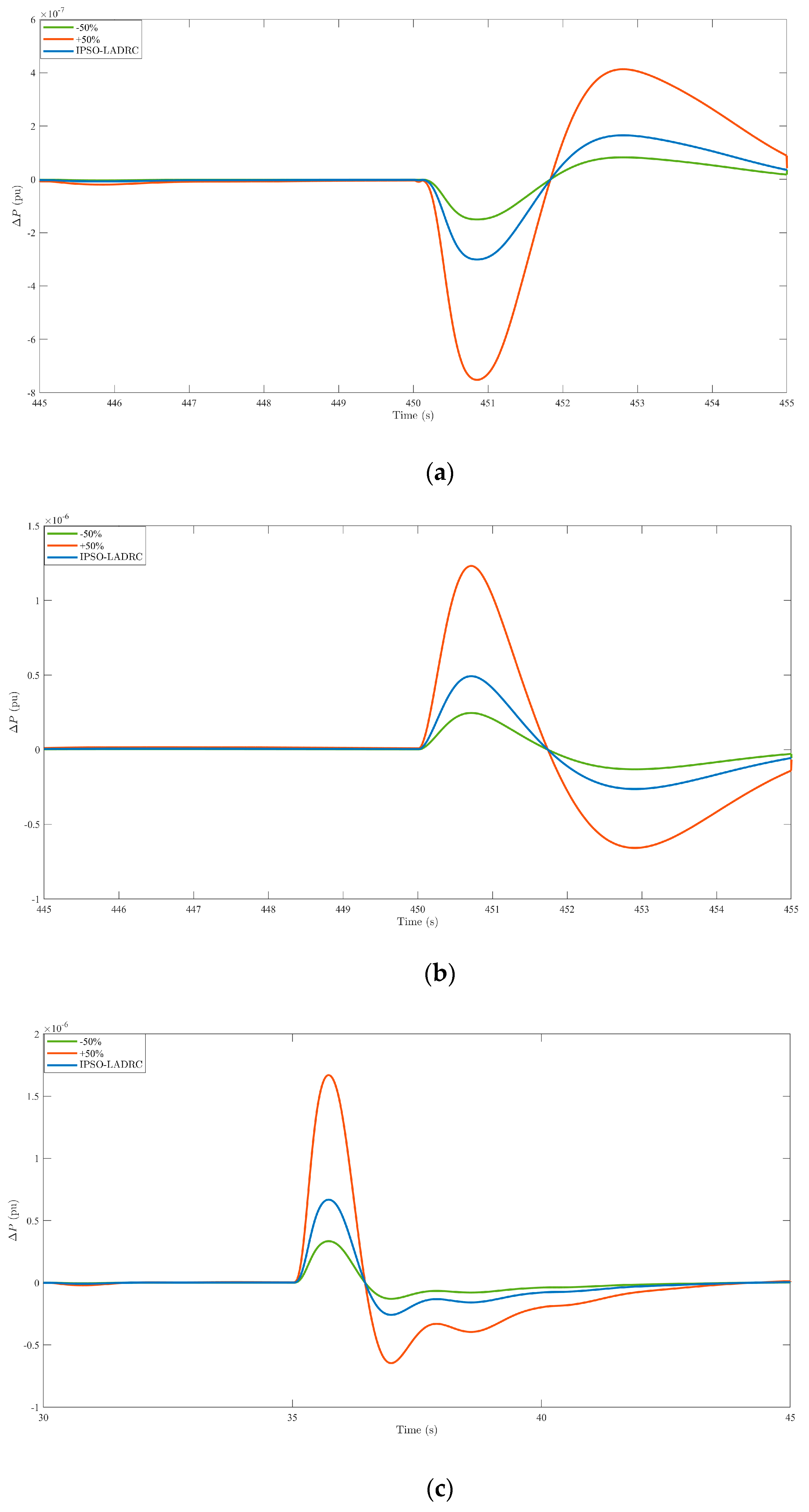
In order to verify the anti-interference ability of the designed controller, this paper increases the parameters in the three-region interconnected power system by 50% and reduces them by 50%, respectively, and randomly selects the parts with larger disturbances for simulation analysis. The simulation results are shown in
Figure 13 and
Figure 14.
It can be seen from
Figure 13 and
Figure 14 that no matter whether the system parameters increase by 50% or decrease by 50%, the system frequency deviation and tie line exchange power deviation will change to a certain extent, but the amplitude of the change is relatively small. It does not affect the normal operation of the system. It can be seen that when the system parameters change to a certain extent, the IPSO-LADRC controller proposed in this article can show good robustness, and, at the same time, it once again proves the good control performance of the controller proposed in this article.
To sum up, in the load frequency control of the three-region interconnected power system proposed in this article, compared with the standard PSO-optimized LADRC, the LADRC controller optimized by IPSO has obvious improvements in anti-interference performance and dynamic characteristics. At the same time, the addition of the IPSO algorithm also makes the parameter tuning of LADRC more convenient and efficient, thus demonstrating the strong practical value of this method.
6. Conclusions
In order to solve the problem of LFC decline caused by the uncertainty of renewable energy output in power system operation, this paper uses LADRC, which has strong anti-interference ability and is independent of the object model, as the load frequency controller of the interconnected power system model; it also proposes an improved PSO with global search capability is to optimize the parameters of LADRC. The improved PSO solves the premature phenomenon in the PSO optimization process and the problem of easily falling into local optimality by introducing Levy flight and Tent chaos mapping, and has been tested in benchmark tests. The effectiveness of the algorithm is verified in the function.
Then, the controller optimized by the improved algorithm is applied to the load frequency control model of the three-region interconnected power system, and the load disturbance is simulated on the Matlab/Simulink platform. The simulation results show that the controller optimized by the improved algorithm greatly reduces system frequency deviation and line exchange power deviation, thus demonstrating the good control effect of the improved algorithm. In addition, in order to verify that the controller optimized by the improved algorithm has strong anti-interference ability, this paper increases the parameters in the three-region interconnected power system by 50% and reduces them by 50%, respectively, and randomly selects the parts with larger disturbances for comparison. Analysis and simulation results show that when the system parameters change to a certain extent, the system frequency deviation and tie line exchange power deviation do not change significantly. It can be seen that the controller optimized by the improved algorithm obviously has strong anti-interference ability.


