PCA-Based Preprocessing for Clustering-Based Fetal Heart Rate Extraction in Non-Invasive Fetal Electrocardiograms

Abstract

Non-invasive fetal electrocardiography (NI-ECG) is based on the acquisition of signals from electrodes on the mother’s abdominal surface. This abdominal ECG (aECG) signal consists of the maternal ECG (mECG) along with the fetal ECG (fECG) and other noises and artifacts. These records allow the acquisition of valuable and reliable information that helps ensure fetal well-being during pregnancy. This paper proposes a procedure based on principal component analysis (PCA) to obtain a single-channel master abdominal ECG record that can be used as input to fetal heart rate extraction techniques. The new procedure requires three main processing stages: PCA-based analysis for fECG-component extraction, polarity test, and curve fitting. To show the advantages of the proposal, this PCA-based method has been used as the feeding stage to a previously developed clustering-based method for single-channel aECG fetal heart rate monitoring. The results obtained for a set of real abdominal ECG recordings from annotated public aECG databases, the Abdominal and Direct Fetal ECG Database and the Challenge 2013 Training Set A, show improved efficiency in fetal heart rate extraction and illustrate the benefits derived from the use of such a master abdominal ECG channel. This allows us to achieve proper fetal heart rate monitoring without the need for manual inspection and selection of channels to be processed, while also allowing us to analyze records that would have been discarded otherwise.

1. Introduction

An essential part of modern obstetric services is electronic fetal monitoring (EFM), which allows diagnosis of fetal distress (FD) during pregnancy. Early detection of any cardiac condition is key to the prevention of after-birth complications or, even, permanent or fatal damage to the newborn’s heart [1,2]. For example, fetal hypoxia is an FD associated with severe perinatal morbidity and mortality, and it is due to an alteration in the placental function that reduces oxygen delivery to the fetus. Thus, the need to prevent heart diseases such as fetal hypoxia has led to the development of different techniques for heart monitoring. However, while this is a well-defined field for adult subjects, fetal monitoring during pregnancy remains a challenge.

Auscultation, cardiotocography (CTG), echocardiography, and phonocardiography (PCG) are the most used methods in clinical practice for continuous fetal heart rate (fHR) monitoring [3,4,5], but those methods have some disadvantages such as their high sensitivity to different types of noise generated by maternal movements and artifacts [6]. However, even if those techniques, and others based on them, are the most used, they do not suffice to give a conclusive diagnosis due to their limited accuracy (even leading to unnecessary cesarean sections [7]). Even if CTG has been considered for years a standard of care for intrapartum fetal surveillance, its data interpretation will always depend on the expert’s judgment and medical diagnosis abilities, since it is based on a visual recognition of the fHR patterns (bradycardia, accelerations, decelerations, etc.), which limits its medical use [8]. This has caused a growing interest in fetal electrocardiograms (fECG), which have become a promising EFM method. The main reason for this is that the fECG signal carries valuable information, such as changes in the morphology of the fECG waveform associated with dysfunctions induced by FD [7]. A way to acquire a fECG is the use of a scalp electrode placed on the head of the newborn during labor, but this is a very invasive method. Thus, non-invasive options for fECG acquisition (NI-fECG) during pregnancy and/or labor have been developed [1]. They make use of some electrodes placed on the maternal abdomen, so each one of these electrodes provides a channel to analyze. While EFM techniques have been shown to help decrease perinatal mortality and morbidity [9] and cesarean sections [10], NI-fECG can offer superior accuracy and reliability than monitoring based on ultrasound technology, and is less likely to display the maternal heart rate in place of the fetal heart rate [11]. Moreover, NI-fECG does not appear to be influenced by increased body mass index or fetal movement, and its high accuracy of heart-rate indices is promising for NI-fECG usage in remote settings [12]. As a matter of fact, results in [12] suggest that, regardless of signal loss, a trace where at least 10 min of fetal R waves are captured that demonstrate physiological FHR indices by displaying normal key FHR parameters such as short-term variation (STV), should be sufficient to demonstrate fetal wellbeing according to the Dawes–Redman criteria [13]. Additionally, NI-fECG devices deliver no energy and women can potentially wear monitors for longer durations without safety concerns, thus effectively enabling long-term monitoring. However, due to the noise produced by the mother’s and fetus’ movements and other artifacts, the resulting abdominal ECG (aECG) record may be seriously affected, resulting in signals either partially distorted (in some of the channels or in fragments of them) or even completely unusable. The extraction of fHR or other characteristics of the fECG signal thus requires sophisticated signal processing in order to overcome this [14,15,16]. As an example, in [14], a clustering-based method for single-channel fetal heart rate monitoring from aECG was presented. However, in that proposal, not all the channels in aECG recordings could be successfully processed due to artifacts, excessive noise, saturation, etc. In some cases, even complete recordings were useless for fHR extraction as none of their channels allowed the identification of ECG characteristics.

The aim of this research is focused on procedures for fHR extraction from NI-fECG recordings that enhance the performance of, in general, previous methods for fHR extraction and, more specifically, those based on clustering [14]. This improvement is oriented to avoid discarding some fragments of channels in aECG recordings, or even complete channels, due to noise or severe artifact contamination. The final objective is to achieve high accuracy in fHR extraction from any aECG recording, with no need to inspect and select channels or fragments. For this purpose, a representative signal of all the channels in an aECG recording will be composed, in which the noises and artifacts that may affect some channels are minimized or even removed. Principal component analysis (PCA) can be used for this task, since PCA is a technique that can reduce the dimensionality of large data sets by transforming a large set of variables into a smaller one that still contains most of the original information. Thus, in this paper, we propose the use of a PCA-based algorithm to extract a single master signal from the aECG recording, which is then fed to the clustering-based algorithm proposed in [14]. fHR results from annotated public aECG databases show the benefits associated with this new framework. The rest of the manuscript is organized as follows: Section 2 describes the background of the different techniques and algorithms. Section 3 is devoted to the description of the proposed algorithm. Results and discussion are presented in Section 4, while the final Section 5 summarizes the main conclusions of this work.

2. Background

The fetal heart rate undergoes dynamic variations, reflecting both physiological and pathological influences. fHR changes not related to physiological events may be a sign of pathologies such as fetal hypoxia, so it is a priority to research how to monitor fHR, fetal movements, and uterine contractions simultaneously. In the following, some concepts in this field are summarized, along with the fundamentals of fECG signal processing.

2.1. NI-fECG Fundamentals

The ECG is an important technique whose acquisition on the human skin involves the reading of very low voltages generated by the heart activity. These signals are contaminated by different sources of noise, and the difficulty is increased when the acquisition target is the fECG signal. The fHR can be obtained from fECG signals [14,17,18,19], and its monitoring is one of the most important methods to detect and identify diseases in the early stages of pregnancy [20]. As was commented above, the NI-fECG is a non-invasive method that consists of the use of a set of surface electrodes placed over the mother’s abdomen in order to acquire the aECG, which is composed of the fECG along with the maternal ECG (mECG). Examples of electrode positioning can be found in [1,2]. One of the main advantages of this non-invasive method is the fact that the fetus is not stressed during the acquisition of the signal, and it allows long-term monitoring during pregnancy [2]. Another advantage of NI-fECG is the absence of any radiated energies, which are mostly present in other methods such as X-rays and ultrasound; although the latter has been shown to be safe for fetal monitoring, prolonged exposure to ultrasound can heat fetal tissues [21]. Moreover, to obtain fECG signals from aECG signals it is important to consider that they are affected by different types of electrical interferences, such as other electric biological signals (mother’s respiration and contractions, fetus’ movement) and external electric artifacts (power line interferences, etc.). In addition, movements at the electrodes and a strong maternal component [22] compared to the weak fetal component may complicate fECG detection. Figure 1 shows an example of a channel of an aECG recording, where these interferences can be observed.

NI-fECG acquisition is usually performed according to two aECG acquisition procedures [23]: the first one is called abdominal electrode sources (AES), which only makes use of the leads placed on the maternal abdomen; meanwhile, the second procedure is called combined source (CS) because, apart from the leads placed on the maternal abdomen, at least an extra lead is placed on the maternal chest to capture the actual mECG signal. This last type of system usually includes an adaptative algorithm that, using those extra leads on the chest, tries to cancel the maternal component, which is the main and most challenging artifact in the aECG mixture [2] for fHR extraction. The relative weakness of the fetal signal and the noisy environment due to the different artifacts mentioned above may make the use of NI-fECG difficult for detecting structural defects of the fetal heart. However, it is possible to extract the fHR, and it is feasible to evaluate the blood conduction velocity, or the condition of tissues within the heart as well as various abnormalities [2]. In any case, the identification of QRS complexes and R-R intervals allows for monitoring heart rate variability. Thus, NI-fECG is an ideal tool for long-term FHR monitoring [22].

2.2. Processing of NI-fECG

Different techniques for processing and extracting characteristics from aECG recordings are found in the literature [7,24,25,26,27]. As it was mentioned above, the fECG is mixed with other biopotentials and noises, such as the mECG, respiratory artifacts and contractions [1], and even the movement of the fetus or the mother, and it is very important to consider them as one of the main problems in the analysis of aECG records. Sudden movements from the fetus or the mother can even lead to saturation in the recordings. Additionally, some of these artifacts result in baseline wandering (BW). Wavelet denoising has been shown to be a useful tool for the removal of these artifacts, even suitable for implementation on embedded hardware [16,28]. Other methods of adaptive noise cancellation are least mean square (LMS) and Widrow’s multireference [29,30,31]. On the other hand, techniques based on wavelet transforms (WT) [22,32,33,34], empirical mode decomposition (EMD) [18,19,35], Kalman filtering [25,36], artificial neural networks [37,38,39], adaptative filtering [40,41,42], blind source separation [7,26,30,43], or even clustering-based algorithms [14], have been shown to be useful in the extraction of components more suitable to obtain relevant characteristics of the fECG, such as R-peak locations. The techniques to denoise aECG signals and to extract reliable fetus information used in this work are summarized in the following.

2.2.1. Wavelet Denoising

The aim of aECG denoising is to recover a clean signal from the original aECG data, allowing further processing such as separation of the mECG and fECG signals, QRS complex detection, or parameter estimation (fHR, for example). The wavelet transform is one of the most used tools in signal processing and is an effective way to digitally remove noises within specific sub-bands for aECG signals [16]. This wavelet-based approach is used to remove the low frequency trend of a signal, but it introduces no latency and less distortion than digital filter-based approaches. In this way, an adequate wavelet decomposition can be used as a preprocessing method for BW and noise suppression in aECG signals. Moreover, due to the similar wavelet structure for the application of BW and noise suppression, it can be carried out with only one-step wavelet [14,16,22], which enhances efficiency without compromising accuracy, thus saving resources and facilitating hardware implementations [22].

In the following, the application of the wavelet preprocessing approach consists of a wavelet decomposition down to L levels, with the approximation coefficients at level L replaced by an all-zero vector. Additionally, for each level from $i=1$ to M (with $M<L$), the appropriate threshold limit and rule are applied to the detail coefficients. The wavelet reconstruction based on the zeroing approximations of level L, the modified details of levels 1 to M, and the original details of levels $M+1$ to L are computed to obtain the BW-corrected and denoised aECG signal [14,16,22].

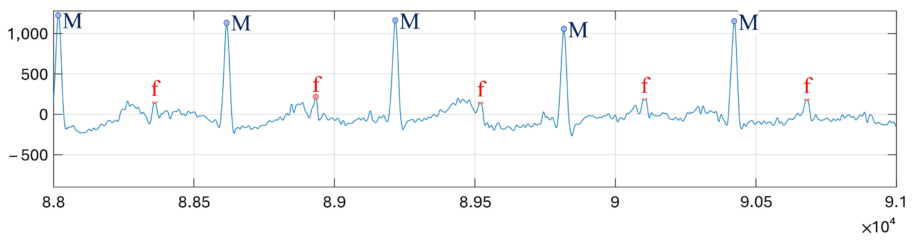
2.2.2. Clustering-Based Procedure for FHR Extraction

Cluster analysis is one of the most used statistical methods to separate objects with the same characteristics in diverse groups (called clusters, defined as groups of similar objects that differ from objects in other groups), and is mainly used in data mining and as an unsupervised learning technique for the classification of objects into clusters [14,44]. Thus, clustering can be used to classify distinctive features of denoised aECG signals in order to separate fetal from maternal QRS complexes. After that, fetal QRS complexes can be used for fHR monitoring.

The clustering-based method proposed in [14] uses for this classification the so-called candidate RS-peaks, which are local maxima followed by a local minimum. Concretely, the clustering algorithm comprises two stages: the first stage carries out the detection of maternal and fetal QRS combining the use of thresholds and clustering itself, while the second stage corrects false negatives (FN) and false positives (FP). In the first stage, the maternal and fetal QRS (mQRS and fQRS, respectively) detection is based on the location of candidate RS-peaks. These are local maxima followed by a local minimum in the preprocessed aECG signal. These RS-peaks correspond to two possible scenarios [14], depending on whether or not the amplitudes of the fetal RS waves are similar to the amplitudes of the maternal RS waves, which should be normally larger. When these amplitudes are comparable, an additional feature is required to differentiate maternal and fetal candidates, which is the product of the amplitude and time distance of the candidate peak, rather than the amplitude. Thus, a smoothed version of the normalized distribution of the amplitudes of all candidate peaks in the classification window is classified into three possible cases, depending on the number of local maxima in this distribution [14]:

• Case 1: detection of two local maxima from the first local minimum, which represents candidates that are actually noise. Each of these maxima provides information about the amplitude zones corresponding to fetal RS-peaks and maternal RS-peaks. If the distance between these maxima is 35% greater than the maximum candidate amplitude, maternal candidates are larger than fetal ones and amplitudes are the selected data to be classified.
• Case 2: detection of two local maxima from the first local minimum, the distance between which is 35% less than the maximum candidate amplitude. This situation can be related to similar amplitudes for fetal and maternal RS-peaks and, thus, amplitudes multiplied by the number of samples of the candidates are the data to be classified.
• Case 3: detection of a single local maximum from the first local minimum. This situation generally corresponds again to similar amplitudes for fetal and maternal RS-peaks, and amplitudes multiplied by the number of samples of the candidates are the selected data to be classified.

Once the case and, thus, the data to be classified are determined, the candidates are classified using the k-medoids++ clustering algorithm into three groups: maternal R peaks, fetal R peaks, and noise. After this classification, the second stage of the FHR monitoring includes a method for the detection of FNs, non-detected fQRS complexes, and FPs, false-detected FQRS complexes [22]. For this, several RR time distances are defined for each fQRS candidate to preceding and succeeding candidates, so FPs and FNs are detected imposing limits to the beat-to-beat variability of the detected heart rate [22].

Compared to threshold-based methods [22,45], clustering allows better detection of fetal QRS complexes since it is less affected by the amplitude variation of the R peak. In some cases in [14] all the channels in a given recording can be analyzed, but in most recordings, one or several channels were discarded due to the quality of the aECG. Thus, while the algorithm in [14] is able to successfully extract the fHR, it still presents some disadvantages, especially the need to preselect those channels in the recording that are apt for analysis, which usually requires a specialist and is not a trivial task to be automatically carried out. Thus, the objective of this work is to enhance the performance of the cluster algorithm in [14] for fHR extraction, which will be used to evaluate a single master channel obtained through a PCA-based algorithm of the complete aECG recording.

2.2.3. Blind Source Separation Fundamentals

Blind source separation (BSP) methods have been widely used in the past, and they have been successfully used in fECG extraction [7,27,30,43,46,47]. The principle of these methods is the decomposition of the signal mixture (aECG) into the original source components (fECG, mECG, and noise), assuming that these components are statistically independent. BSP techniques involve statistical methods such as PCA, independent component analysis (ICA), and singular value decomposition (SVD) [23,48]. These methods have been proven to be suitable for fECG extraction from a multichannel aECG but, nevertheless, a larger number of input signals is associated with greater computational complexity and lower comfort for the pregnant subject during monitoring [7]. In any case, recordings with more channels will provide more accurate data. Our proposal is based on PCA, whose fundamentals are presented in the following.

2.2.4. Principal Component Analysis (PCA)

PCA is a powerful tool for data analysis, as it finds patterns in data of high dimensionality. It allows us to identify patterns in data and to highlight their similarities and differences, since in other methods these patterns may be hard to find in data of many dimensions [40]. The other main advantage of the PCA method is that, once data patterns are found, data can be compressed, i.e., the number of dimensions can be reduced without significant loss of information [23]. Considering the application of PCA methods to aECG signals, they allow us to combine all channels [40] into a reliable single signal. To perform the PCA analysis, the cross-correlation matrix between input signals is built, eigenvalues and eigenvectors are computed and, finally, input signals are transformed according to the eigenvectors and eigenvalues [40]. The covariance matrix, $m{t}_{cov}$, can be calculated as:

$$m{t}_{cov}[x_i,x_j]=E(x_i-E\left[x_i\right]){(x_j-E\left[x_j\right])}^T$$

(1)

where x is the array with the values to be analyzed, E denotes the expected value (mean), and T is the symbol of the transposed matrix. Let e$vecto{r}_k$ be the k-th eigenvector and $evalue{s}_k$ the corresponding eigenvalue of $m{t}_{cov}$. Then, the k-th principal component is obtained using the following expression:

$$y_k=evecto{r}_k^{T}x$$

(2)

The spread of the eigenvalues is a good indicator of how many principal components are of real interest in our input data, so the signals associated with small eigenvalues are usually dropped. As a result, we will have one or more components that represent the input signals in a minimum mean square sense. The principal components capture the power of most of the signal and, at the same time, all components are orthogonal to each other. That is why PCA sometimes is also called a whitening operation [15,40,49]. Thus, the PCA method fits perfectly with one of the main objectives of this work, which is the generation of a single aECG master signal without discarding any of the original channels from the aECG recording, in order to subsequently apply techniques for the extraction of fetal information of interest such as the fHR.

3. Proposed Framework

As discussed extensively above, NI-fECG consists of a set of multiple signals obtained with electrodes placed on the maternal abdomen. Usually, most proposals to extract the fetal characteristics [7,14,15,48] require the search for the channel or channels from the aECG with less noise contamination, discarding even fragments of some channels when they are affected by severe artifacts [40], and even discarding complete aECG recordings. Thus, removing or discarding any channel could remove vital information about the fetus. The proposed PCA-based algorithm seeks to solve this problem and to prevent a complete record, signal, or fragment from being discarded. With that aim, a PCA-based [15,23,27,40] algorithm is proposed, which will extract a single aECG master signal from the aECG record without discarding any of its channels. This master signal will be fed to the clustering algorithm in [14] to extract the fetal QRS complexes and, thus, monitor fHR. The proof of concept has been implemented using GNU Octave 8.4 and Python 3.12, due to library compatibility, and then trained and tested using aECG recordings in two PhysioNet databases [50]. These databases are described below, while the new procedure will be detailed in Section 3.2.

3.1. Fetal ECG Datasets

PhysioNet [51] offers free and public web access to large collections of recorded physiologic signals (PhysioBank), and the included databases are made available under the ODC Public Domain Dedication and License v1.0 [52]. Concretely, two of these databases provided by PhysioNet have been used for this work:

• Abdominal and Direct Fetal Electrocardiogram Database (ADFECGDB) [50]: this database contains multichannel fECG recordings obtained from five different women in labor. Each recording comprises four 5 min differential signals acquired from the maternal abdomen, and the reference direct fECG registered from the fetus head. The recordings are sampled at 1 ksps with 16-bit resolution, and the signal bandwidth is 1–150 Hz. Moreover, the database includes a set of reference annotations indicating the fetal R-wave locations. The ADFECGDB will be used to train the proposed algorithm.
• Challenge 2013 Training Set A (Challenge) [53]: these data consist of one-minute fECG recordings, sampled at 1 ksps, each one including four noninvasive abdominal signals as well as the reference annotations marking fetal R-wave locations [14]. The Challenge database is used to test and validate the proposed algorithm.

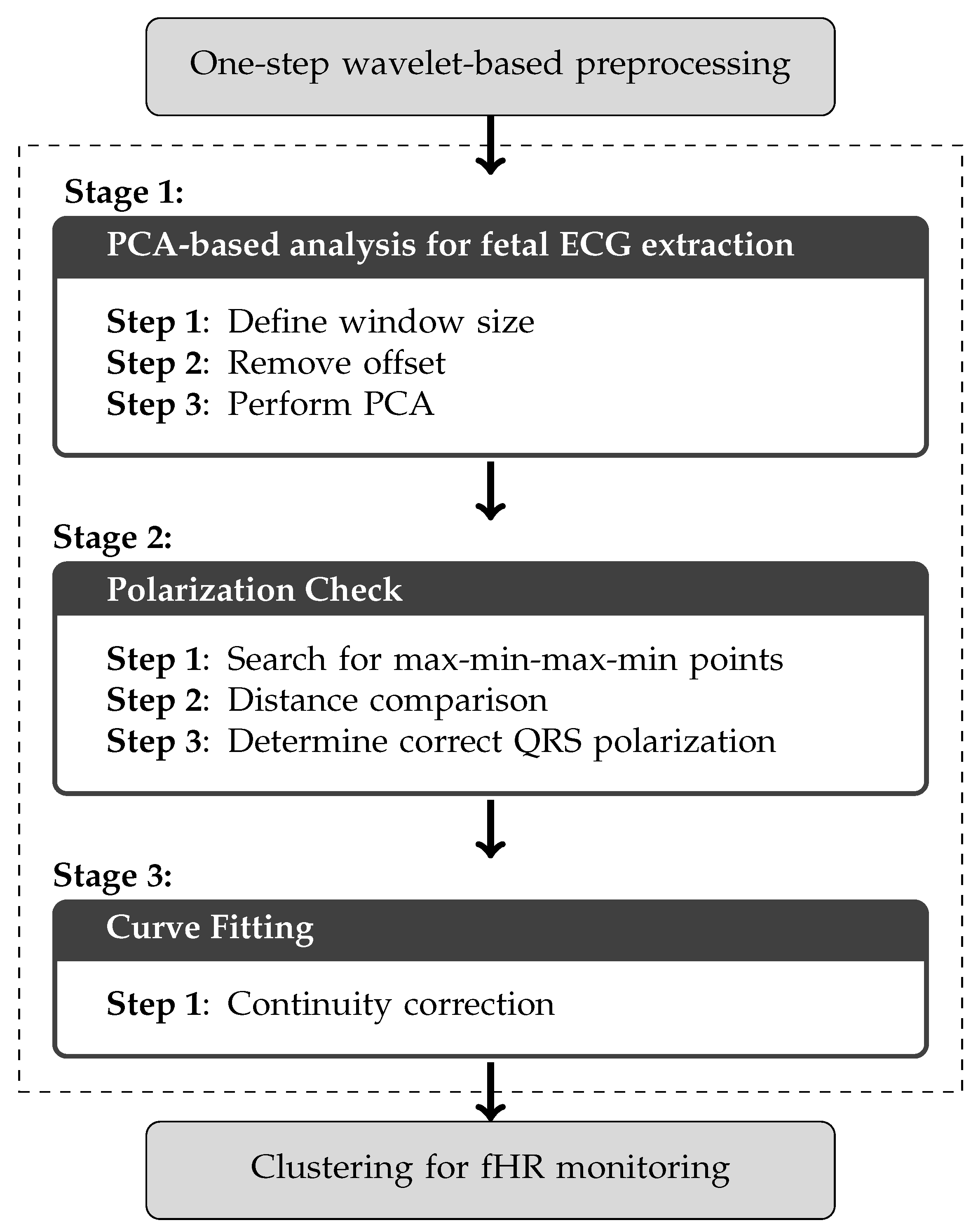
3.2. Proposed PCA-Based Framework

As it was commented above, the objective of this work is to generate, through a PCA-based algorithm, an aECG master signal from the different channels in an aECG recording. As it is common practice in many digital signal processing algorithms, the signals will be divided into windows. Thus, the size of these windows must be adjusted to provide a correct analysis as well as to minimize the delay between acquisition and processing. It is also important to take into account that window-based processing can produce non-continuous signals, while it is also possible to have opposing polarities in adjacent windows as a result of differing signs in the eigenvalues. Considering all these aspects, this work proposes to track the signal obtained after the PCA analysis in order to perform a polarity check followed by a curve fitting. A schematic of the proposed PCA-based framework is shown in Figure 2: PCA-based analysis, polarity check, and curve fitting. These stages and their steps are described in detail below, keeping first in mind that the aECG signals to be processed will have been preprocessed using the one-step wavelet-based algorithm described in [16]. Figure 3 illustrates a fragment of the r01 record from the ADFECGDB training set before and after this wavelet-based preprocessing. The parameters [16] for the wavelet preprocessing stage of the databases used in this work were: wavelet function Daubechies 6, L = 7 (due to the maximum frequency component of the signals), M = 3, universal threshold, multiple rescaling, and soft thresholding.

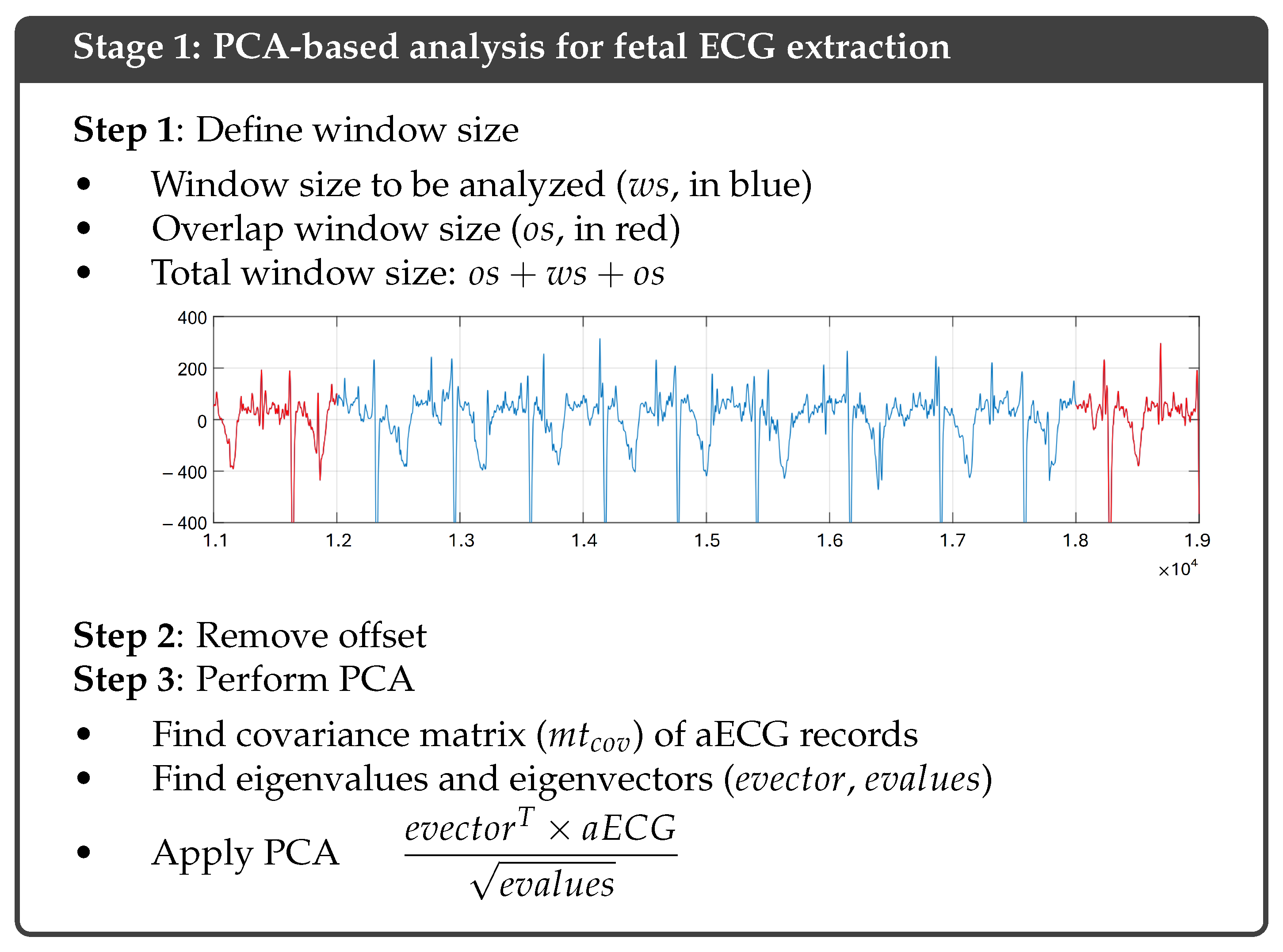
3.3. Stage 1: PCA-Based Analysis for Fetal ECG Extraction

Due to the presence of artifacts in aECG signals, many works in the literature [14,15,23,27,35,40] usually discard a fragment of a channel from aECG recordings, a complete channel, or even all of them, when extracting fetal characteristics such as fHR. Therefore, the application of the proposed PCA-based algorithm before extracting any information allows us to obtain a master aECG signal as the first principal component using the entire aECG record, including those fragments and channels that might have been discarded in previous models due to noise or artifacts. The application of PCA to the input signal avoids the need for an a priori analysis of the aECG records, searching for fragments in the channels that are not affected by artifacts or other noise. This limits the loss of information and provides a feasible signal for further analysis, even for studies outside of a controlled environment. A complete scheme of this stage with the three necessary steps is shown in Figure 4, while an algorithmic summary is shown in Algorithm 1. This stage is detailed in the following.

Algorithm 1 PCA-based analysis for fetal ECG extraction.

1: Step 1: Define window size 2: if $\mathrm{signal}\mathrm{is}\mathrm{shorter}\mathrm{than}ws$ then            ▹ One-window case 3:     $\mathrm{left}\mathrm{window}\mathrm{extension}\leftarrow 0$ 4:     $\mathrm{right}\mathrm{window}\mathrm{extension}\leftarrow 0$ 5: else if first window then                   ▹ First window 6:     $\mathrm{left}\mathrm{window}\mathrm{extension}\leftarrow 0$ 7:     $\mathrm{right}\mathrm{window}\mathrm{extension}\leftarrow os$ 8: else if last window then                   ▹ Last window 9:     $\mathrm{left}\mathrm{window}\mathrm{extension}\leftarrow os$ 10:     $\mathrm{right}\mathrm{window}\mathrm{extension}\leftarrow 0$ 11: else                           ▹ Any other case 12:     $\mathrm{left}\mathrm{window}\mathrm{extension}\leftarrow os$ 13:     $\mathrm{right}\mathrm{window}\mathrm{extension}\leftarrow os$ 14: end if 15: $aux\leftarrow aECG\left[\mathrm{extended}\mathrm{window}\right(ws,os\left)\right]$ 16: Step 2: Remove offset 17: for $j=1$ to $num\_channels$ do 18:     $aux[j,:]\leftarrow aux[j,:]-$ mean $\left(aux\right[j,:\left]\right)$ 19: end for 20: Step 3: Perform PCA 21: $mt\_cov\leftarrow$cov$\left(au{x}^{\prime }\right)$               ▹ Find covariance matrix 22: $[evectors,evalues]\leftarrow eig(mt\_cov)$    ▹ Find eigenvalues and eigenvectors 23: $pca\leftarrow \left(evalue{s}^{-0.5}\right)\times \left(evector{s}^{\prime }\right)\times \left(aux\right)$              ▹ PCA 24: $Master\leftarrow pca[\mathrm{first}\_\mathrm{principal}\_\mathrm{component},:]$     ▹ aECG master signal

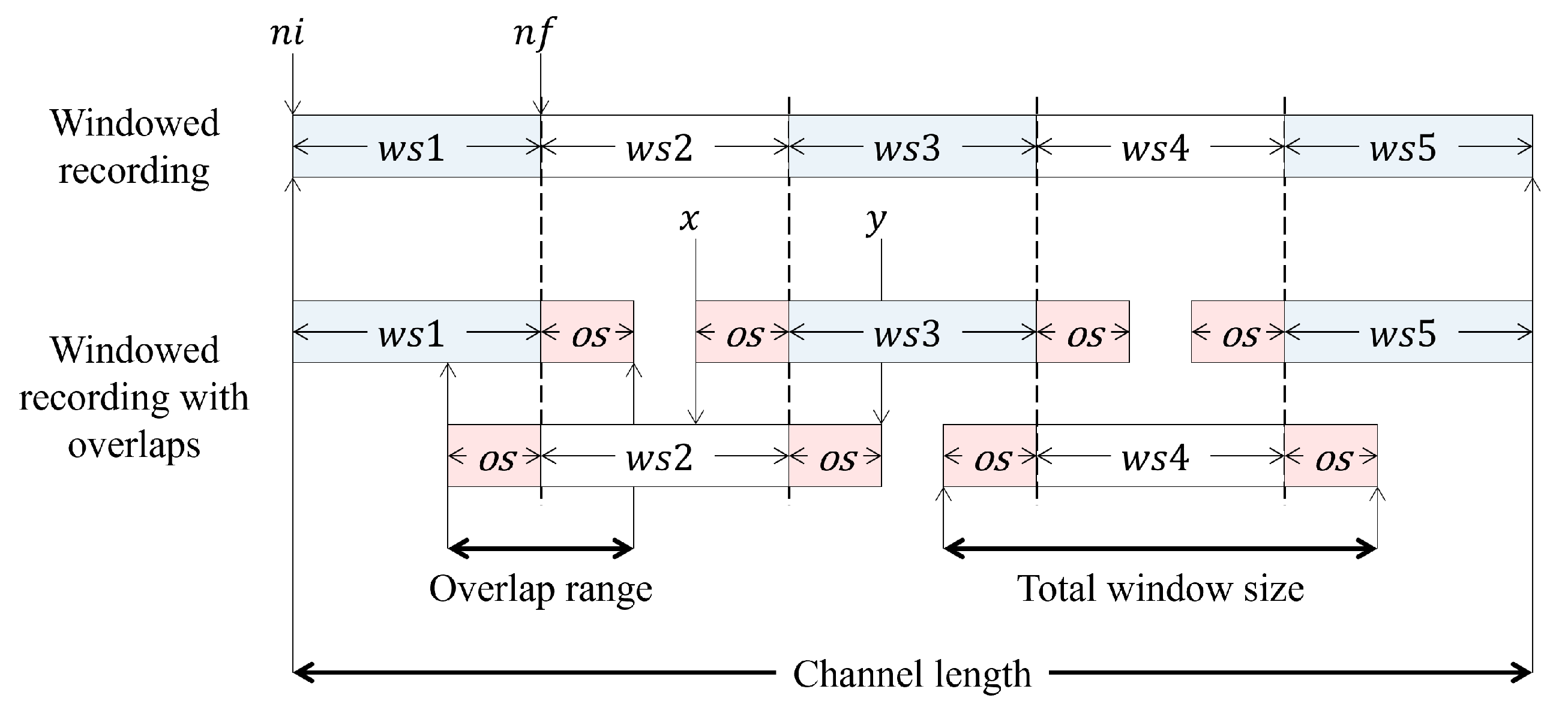
3.3.1. Step 1: Define Window Size

In order to reduce the complexity of the proposed signal processing, especially if its future implementation on wearable devices is sought, it is important to select an appropriate window size ($ws$) that provides a balance between performance (in terms of data rate, resources, and execution time) and the quality of the resulting signal. Since the training database records, PhysioNet’s ADFECGDB [50], have a total of 300,000 samples, window sizes of 6000, 10,000, 12,000, 15,000, 20,000, 30,000, 50,000, 60,000, 100,000, 150,000, and 300,000 samples were considered in order to evaluate the influence of this parameter in the results. An additional parameter to $ws$ is the overlap size ($os$), which will be needed in stage 3. This overlap size defines an overlap region involving the number, $os$, of the final samples of the previously parsed window and an equal amount of the first samples in the window after the current one. Thus, these fragments will be added to the beginning and end of each analyzed window. $os$ should include at least a full heartbeat, so a 1 s, 1000-sample fragment will be considered in this work.

Figure 5a shows an example of how the system, once $ws$ has been defined (in blue, 4000 samples for this example), proceeds to add two new fragments of the signal to both of its ends. We will call these fragments overlaps (in red in the example) and their size is $os$ (1000 samples for this example, the sampling frequency is 1 ksps). The fragments thus added to the current window as overlap corresponds to the final samples of the preceding window, already analyzed, and to the initial samples in the next window to be analyzed. These overlap fragments increase the total size of the window to be analyzed to $ws+2os$. It is important to note that the first window to be analyzed, since this is the one initializing the system, will be only expanded after its final samples with $os$ samples from the second window. In the same way, the last window to be processed will be only expanded at its beginning with $os$ samples from the preceding window. These two windows will thus be the only ones whose size is $ws+os$, as illustrated in Figure 6.

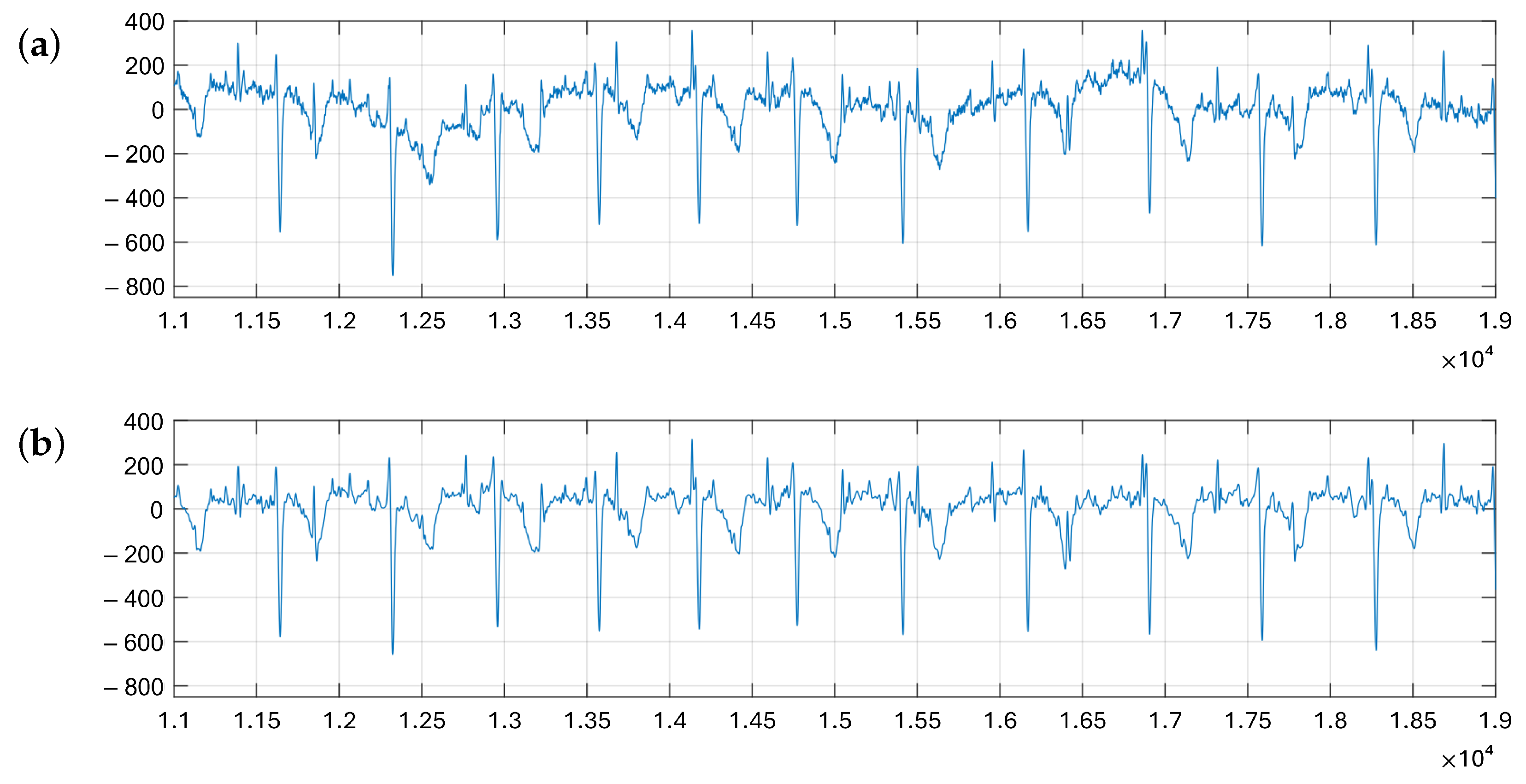
3.3.2. Step 2: Remove Offset

To eliminate the offset, it is necessary to subtract each of the aECG signals from their respective non-zero mean to guarantee a centered PCA signal. If x is one of the aECG channels, including offset, $E\left(x\right)$ is its mean value, and $xc$ is the centered aECG channel, then the i-th samples are related according to:

$$x{c}_i=x_i-E\left(x\right)$$

(3)

3.3.3. Step 3: Perform PCA

This step completes the PCA-based algorithm, which transforms the aECG recording into its principal components, since the aim of PCA is to decorrelate the observed aECG signal using variance as a measure by projecting the data onto orthogonal axis [43]. Thus, after performing the PCA analysis, a master aECG component, i.e., the component corresponding to the larger eigenvalue, will be generated, as illustrated in Figure 5b. It must be noted that no particular consideration about the obtained eigenvalues has been considered, as the scree plot for this type of signal always shows a dominant component, which is the one selected as the master aECG component in this proposal. As will be shown in Section 4, the evaluation of this proposal will be carried out through the fHR performance of this PCA-generated master aECG. Figure 5b shows how noise and artifacts that make parts of channels #1 and #3 unsuitable for fECG extraction are mitigated, and the resulting master aECG component allows us to clearly observe all maternal and fetal beats. Concretely, Figure 7 expands the signals in Figure 5 focusing on a distorted fragment. Thus, it can be seen in Figure 7a how channel #1 of the aECG presents great distortion between samples 88,000 and 90,500, probably due to noise during acquisition. However, the signal obtained from the PCA analysis, in Figure 7b, is suitable for further analysis and fHR extraction, which would not be possible over that particular fragment in channels #1 and #3. Even as some of the distortion is still carried over in the PCA-composed master aECG signal, both maternal and fetal QRS complexes are clearly visible and suitable for extraction.

3.4. Stage 2: Polarization Check

Once the PCA-based algorithm stage is finished, a single master aECG signal can be composed through the concatenation of the resulting windows from the first principal component of all analyzed aECG recordings. However, in very particular cases the polarity of the fQRS and mQRS complexes can be inverted in some windows, due to noise or artifact contamination in a fragment of a channel, a complete channel, or in all the channels of the analyzed window. This must be corrected through the steps shown Figure 8, which will be described below.

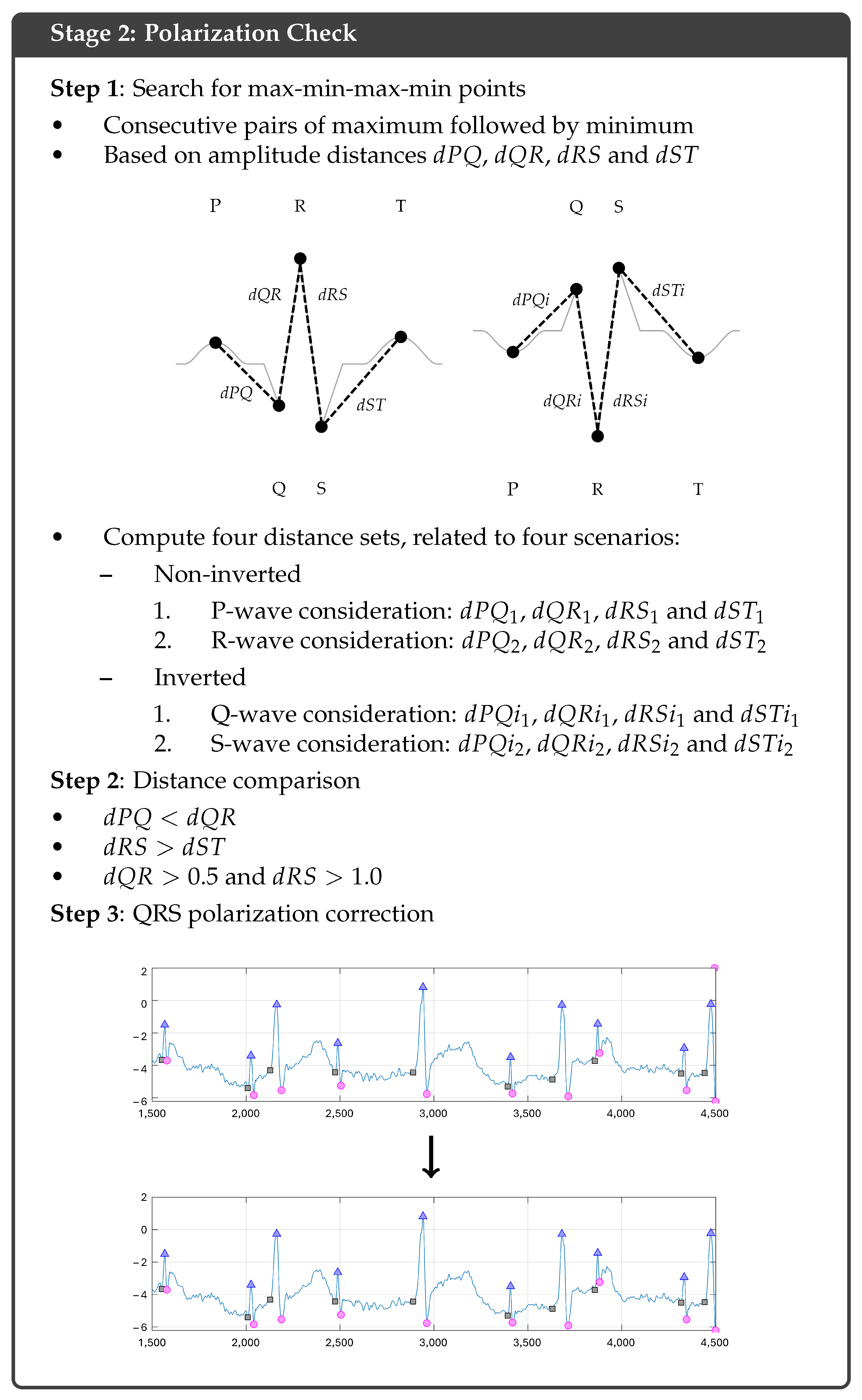
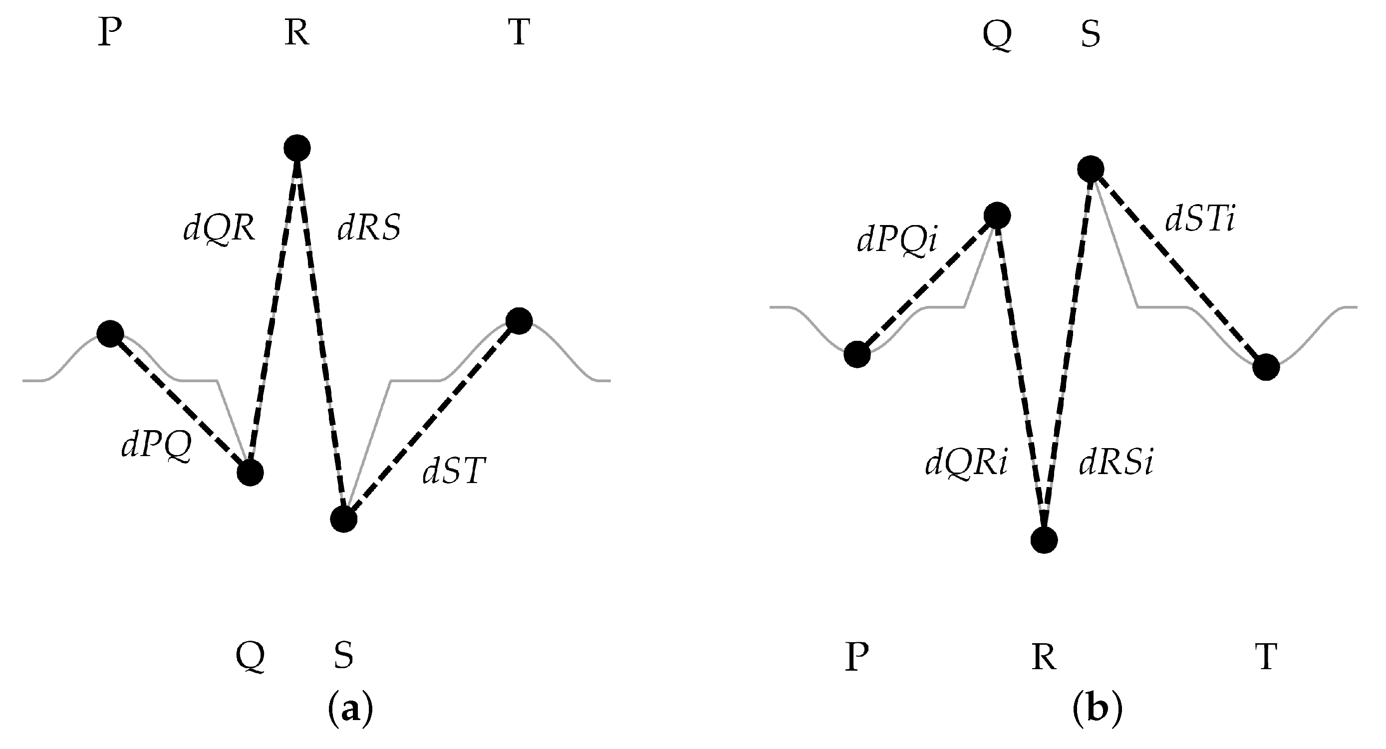
3.4.1. Step 1: Search for Max-Min-Max-Min Points

In this step, a search for local maxima and minima is carried out. This search is intended to determine the correct polarization of the generated master aECG wave. In an ideal case, local maxima could correspond to either P, R, or T waves, while the local minima would match Q and S waves. However, the system cannot determine if the first maximum found is a P, R, or T wave, and it is even possible that the signal has been inverted in the PCA process, with maxima thus corresponding to Q or S waves. Additionally, these maxima and minima may not be related to any cardiac phenomena and will usually correspond to noise or signal fluctuations. In this way, Figure 9 illustrates how a QRS-complex would match the local maxima and minima for the two possible polarities, where $dPQ$ is the amplitude distance between the P and Q peaks, $dQR$ is the amplitude distance between the Q and R peaks, $dRS$ is the amplitude distance between the R and S peaks, and $dST$ is the amplitude distance between the S and T peaks. These distances must satisfy several conditions to match the patterns in Figure 9 and, thus, define a QRS-complex.

Based on the reasoning above, the analysis requires to consider several maxima and minima, with two consecutive pairs of a maximum followed by a minimum grouped together as the core of each iteration. In the following, these will be referred to as $ma{x}_1\left(j\right)$, $mi{n}_1\left(j\right)$, $ma{x}_2\left(j\right)$ and $mi{n}_2\left(j\right)$ for the j-th iteration. This analysis will result in four possible scenarios, two for each possible polarity, when these maxima and minima are related to a PQRST sequence. This will allow us to identify a cardiac component using the $dPQ$, $dQR$, $dRS$, and $dST$ distances under four different sets of assumptions, each corresponding to one of the scenarios described below:

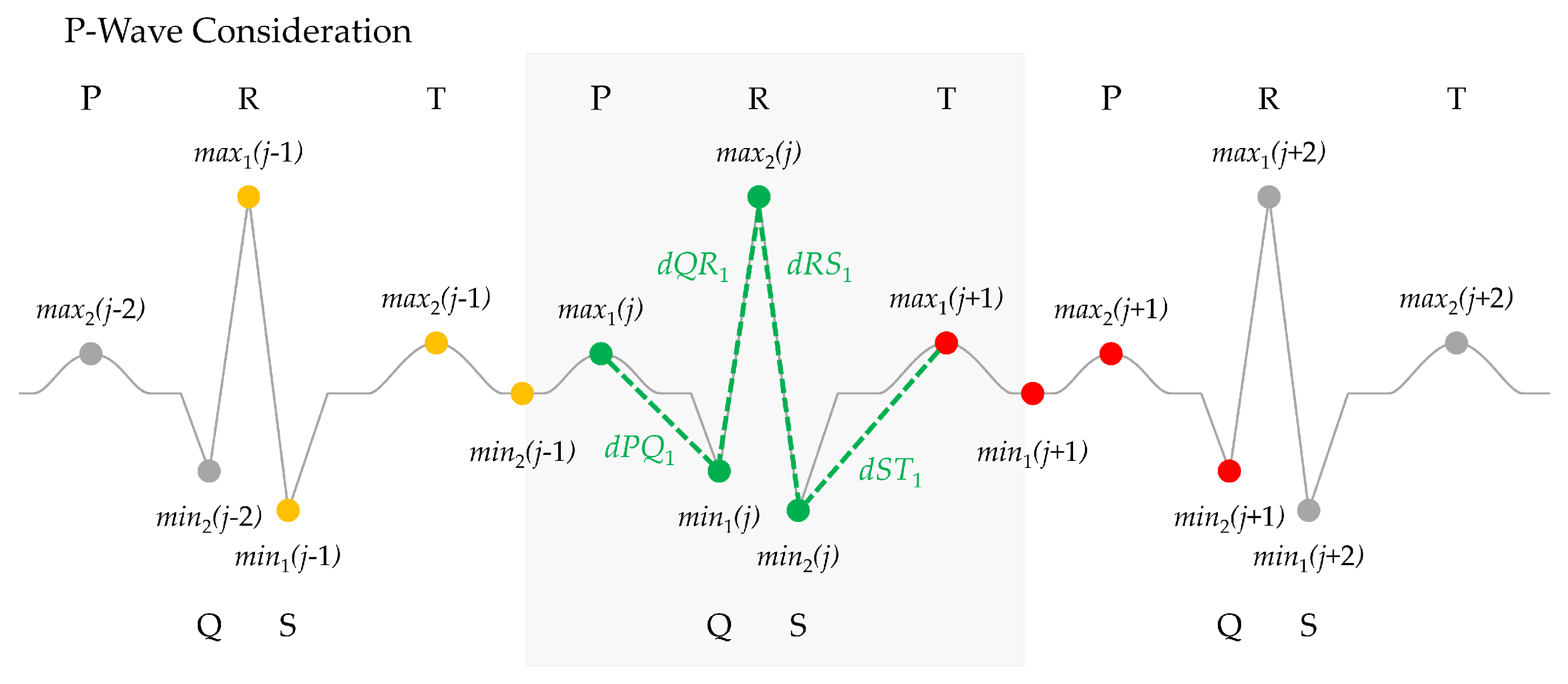
• In the first scenario, it is considered that the first maximum found is the P-wave, located at $ma{x}_1\left(j\right)$, where j is the index of the pair of maximum–minimum being evaluated, as shown in Figure 10. Thus, the next values to be found are the Q wave, located at $mi{n}_1\left(j\right)$, the R wave at $ma{x}_2\left(j\right)$, and the S wave, located at $mi{n}_2\left(j\right)$, while the T wave corresponds to the first maximum of the next group, $ma{x}_1(j+1)$. These allow us to define and analyze the distances $dP{Q}_1$, $dQ{R}_1$, $dR{S}_1$, and $dS{T}_1$ as shown in Figure 10.

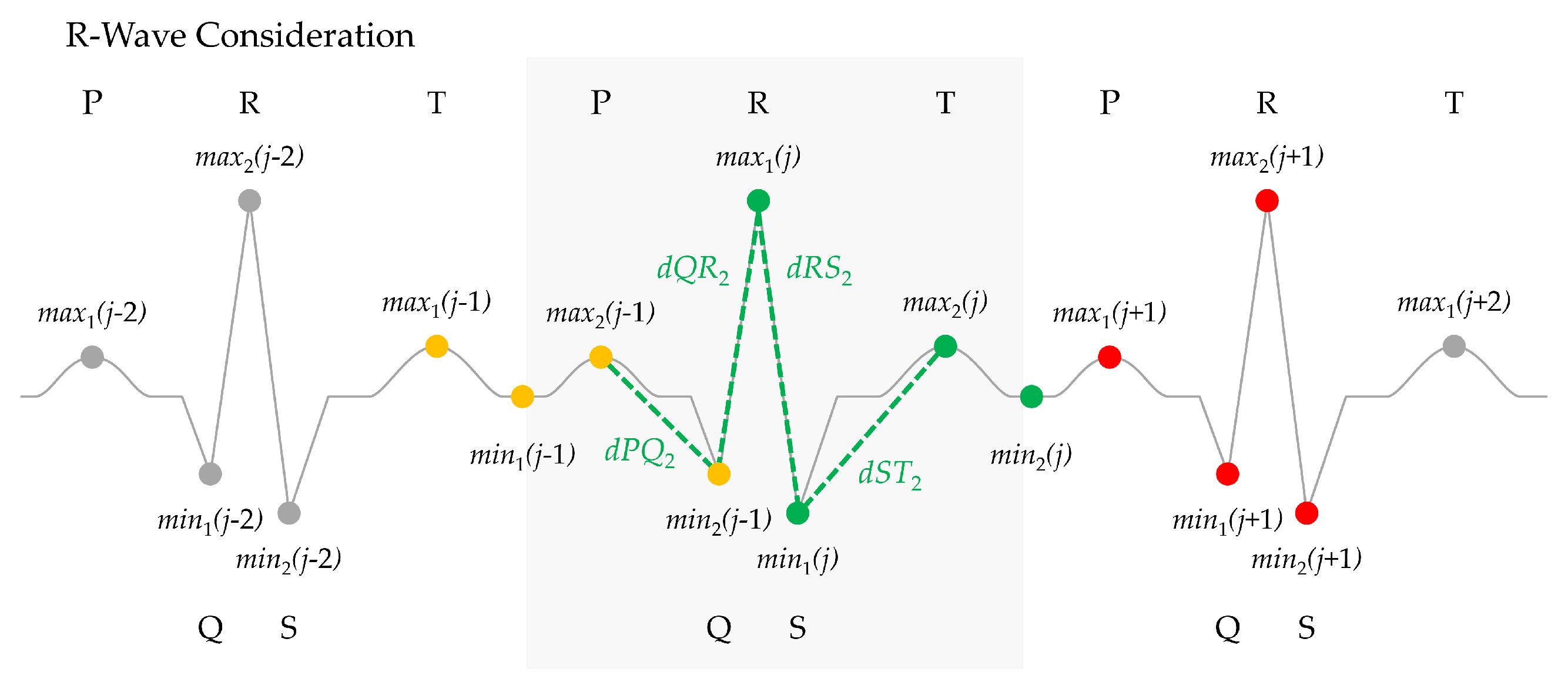
• In a second scenario, it is considered that $ma{x}_1\left(j\right)$ corresponds to a R-wave, as shown in Figure 11. Thus, the set of distances $dP{Q}_2$, $dQ{R}_2$, $dR{S}_2$, and $dS{T}_2$ can be computed as illustrated in Figure 11 using the points $ma{x}_2(j-1)$, which should correspond to the previous P wave, $mi{n}_2(j-1)$, corresponding to the Q wave, $mi{n}_1\left(j\right)$, which should match the S wave, and finally $ma{x}_2\left(j\right)$ as the T wave.

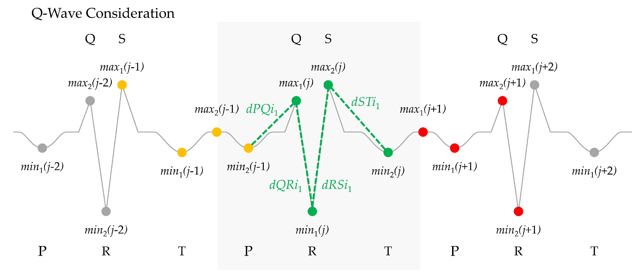
• In the case the polarity is inverted, a third scenario is possible where it is considered that the first maximum found is the Q wave at $ma{x}_1\left(j\right)$, as shown in Figure 12, where it is illustrated how the distances $dPQ{i}_1$, $dQR{i}_1$, $dRS{i}_1$, and $dST{i}_1$ are obtained using the points $mi{n}_2(j-1)$, $mi{n}_1\left(j\right)$, $ma{x}_2\left(j\right)$, and $mi{n}_2\left(j\right)$.

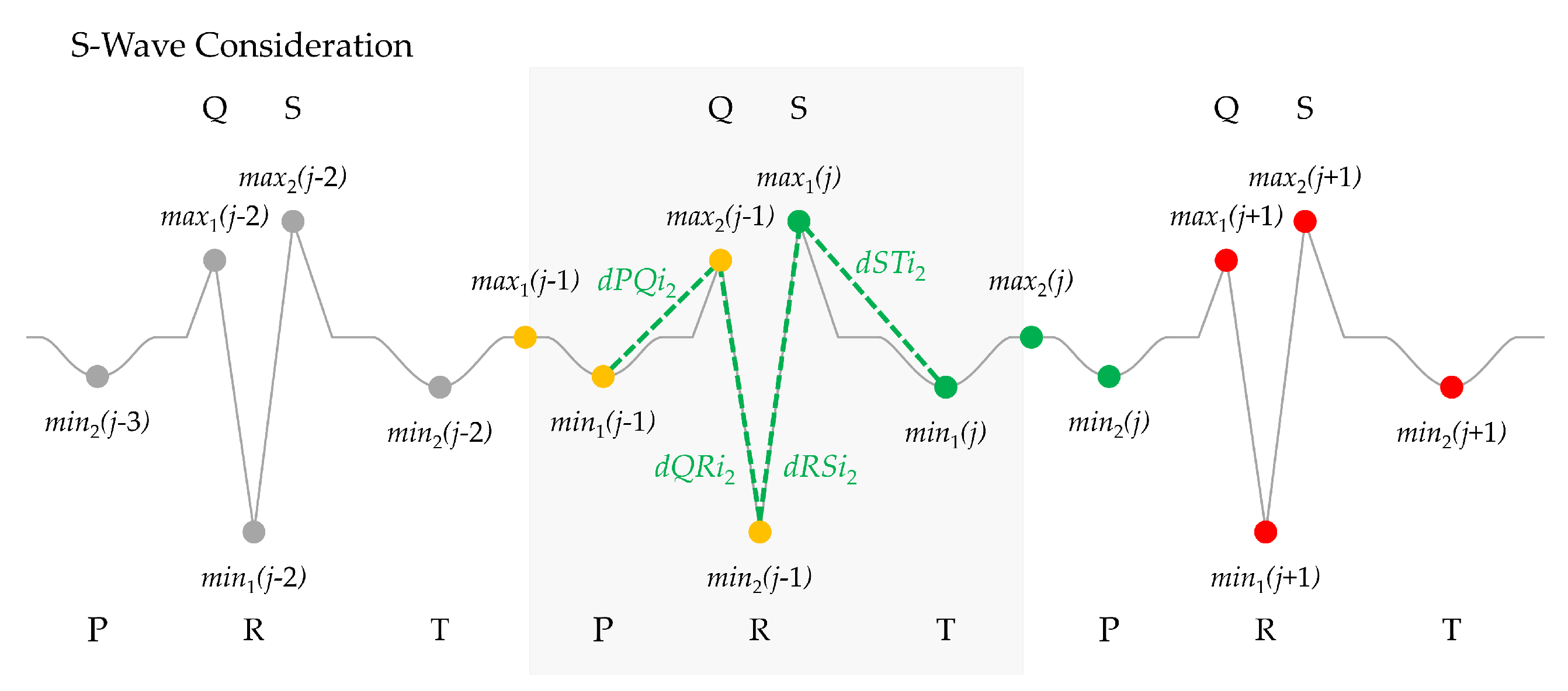
• Finally, when the polarity is inverted, a final scenario is defined in Figure 13, so $ma{x}_1\left(j\right)$ corresponds to the S wave and the set of distances $dPQ{i}_2$, $dQR{i}_2$, $dRS{i}_2$, and $dST{i}_2$ are computed using $mi{n}_1(j-1)$, $ma{x}_2(j-1)$, $mi{n}_2(j-1)$, and $mi{n}_1\left(j\right)$.

It is important to finally note that it is not necessary to include additional scenarios for a possible T wave, since they will result in redundant evaluations. Thus, these four scenarios will suffice to determine the type of wave, as discussed below, that the pair of maxima and minima may match. The pseudocode in Algorithm 2 summarizes this first step of the second stage of the proposed PCA-based framework.

Algorithm 2 Polarization check, step 1.

1: Step 1: Search for max-min-max-min points 2: Consecutive pairs of maximum followed by minimum 3: procedure maxmin($Master$) 4:     $flag\leftarrow 1$, $j\leftarrow 1$ 5:     for $mx\leftarrow 2$ to length$\left[Master\right]$ do 6:         if $\left(Master\right[mx]\ge Master[mx-1\left]\right)$ and $\left(Master\right[mx]>Master[mx+1\left]\right)$ and          $(mx\le$length$\left[Master\right])$ and $(flag=1)$ then               ▹ Find the first maximum 7:            $ma{x}_1\left[j\right]\leftarrow mx$ 8:            $flag\leftarrow 2$ 9:         end if 10:         if $\left(Master\right[mx]\le Master[mx-1\left]\right)$ and $\left(Master\right[mx]<Master[mx+1\left]\right)$ and          $(mx\le$length$\left[Master\right])$ and $(flag=2)$ then               ▹ Find the first minimum 11:            $mi{n}_1\left[j\right]\leftarrow mx$ 12:            $flag\leftarrow 3$ 13:         end if 14:         if $\left(Master\right[mx]\ge Master[mx-1\left]\right)$ and $\left(Master\right[mx]>Master[mx+1\left]\right)$ and          $(mx\le$length$\left[Master\right])$ and $(flag=3)$ then             ▹ Find the second maximum 15:            $ma{x}_2\left[j\right]\leftarrow mx$ 16:            $flag\leftarrow 4$ 17:         end if 18:         if $\left(Master\right[mx]\le Master[mx-1\left]\right)$ and $\left(Master\right[mx]<Master[mx+1\left]\right)$ and          $(mx\le$length$\left[Master\right])$ and $(flag=4)$ then             ▹ Find the second minimum 19:            $mi{n}_2\left[j\right]\leftarrow mx$ 20:            $flag\leftarrow 1$ 21:            $j\leftarrow j+1$ 22:         end if 23:     end for 24: end procedure 25: $$ 26: Based on amplitude distances $dPQ$, $dQR$, $dRS$ and $ST$, 27: compute four distance sets, related to four scenarios 28: procedure QRS($Master$, $ma{x}_1$, $ma{x}_2$, $mi{n}_1$, $mi{n}_2$) 29:     for $j\leftarrow 2$ to length$\left[ma{x}_1\right]$ do 30:         ▹ P-wave consideration 31:         $dP{Q}_1[j-1]\leftarrow Master\left[ma{x}_1\left[j\right]\right]-Master\left[mi{n}_1\left[j\right]\right]$ 32:         $dQ{R}_1[j-1]\leftarrow Master\left[ma{x}_2\left[j\right]\right]-Master\left[mi{n}_1\left[j\right]\right]$ 33:         $dR{S}_1[j-1]\leftarrow Master\left[ma{x}_2\left[j\right]\right]-Master\left[mi{n}_2\left[j\right]\right]$ 34:         $dS{T}_1[j-1]\leftarrow Master\left[ma{x}_1[j+1]\right]-Master\left[mi{n}_2\left[j\right]\right]$ 35:                                       ▹ R-wave consideration 36:         $dP{Q}_2[j-1]\leftarrow Master\left[ma{x}_2[j-1]\right]-Master\left[mi{n}_2[j-1]\right]$ 37:         $dQ{R}_2[j-1]\leftarrow Master\left[ma{x}_1\left[j\right]\right]-Master\left[mi{n}_2[j-1]\right]$ 38:         $dR{S}_2[j-1]\leftarrow Master\left[ma{x}_1\left[j\right]\right]-Master\left[mi{n}_1\left[j\right]\right]$ 39:         $dS{T}_2[j-1]\leftarrow Master\left[ma{x}_2\left[j\right]\right]-Master\left[mi{n}_1\left[j\right]\right]$ 40:                                       ▹ Q-wave consideration 41:         $dPQ{i}_1[j-1]\leftarrow Master\left[ma{x}_1\left[j\right]\right]-Master\left[mi{n}_2[j-1]\right]$ 42:         $dQR{i}_1[j-1]\leftarrow Master\left[ma{x}_1\left[j\right]\right]-Master\left[mi{n}_1\left[j\right]\right]$ 43:         $dRS{i}_1[j-1]\leftarrow Master\left[ma{x}_2\left[j\right]\right]-Master\left[mi{n}_1\left[j\right]\right]$ 44:         $dST{i}_1[j-1]\leftarrow Master\left[ma{x}_2\left[j\right]\right]-Master\left[mi{n}_2\left[j\right]\right]$ 45:                                       ▹ S-wave consideration 46:         $dPQ{i}_2[j-1]\leftarrow Master\left[ma{x}_2[j-1]\right]-Master\left[mi{n}_1[j-1]\right]$ 47:         $dQR{i}_2[j-1]\leftarrow Master\left[ma{x}_2[j-1]\right]-Master\left[mi{n}_2[j-1]\right]$ 48:         $dRS{i}_2[j-1]\leftarrow Master\left[ma{x}_1\left[j\right]\right]-Master\left[mi{n}_2[j-1]\right]$ 49:         $dST{i}_2[j-1]\leftarrow Master\left[ma{x}_1\left[j\right]\right]-Master\left[mi{n}_1\left[j\right]\right]$ 50:     end for 51: end procedure

3.4.2. Step 2: Distance Comparison

Following the considerations above on the four possible scenarios maxima and minima may match, all four sets of amplitude distances described in the previous section are evaluated for each pair of maximum–minimum points. Thus, the $ma{x}_1\left(j\right)$, $mi{n}_1\left(j\right)$, $ma{x}_2\left(j\right)$, and $mi{n}_2\left(j\right)$ points in the j-th pair of maxima and minima, along with any required points from the $(j-1)$-th and $(j+1)$-th set of pairs as illustrated in Figure 10, Figure 11, Figure 12 and Figure 13, are used to evaluate the four different sets of amplitude distances for this j-th pair: $dP{Q}_1$, $dQ{R}_1$, $dR{S}_1$, and $dS{T}_1$ (Figure 10), $dP{Q}_2$, $dQ{R}_2$, $dR{S}_2$, and $dS{T}_2$ (Figure 11), $dPQ{i}_1$, $dQR{i}_1$, $dRS{i}_1$, and $dST{i}_1$ (Figure 12), and $dPQ{i}_2$, $dQR{i}_2$, $dRS{i}_2$, and $dST{i}_2$ (Figure 13). It must be noted that when the pair of maxima and minima does not correspond to any cardiac component but is caused by noise and artifacts, as will usually be the case for most pairs of maxima and minima, none of the amplitude distance sets will match any of the scenarios. For this analysis, a set of conditions and thresholds are thus imposed to all the sets of amplitude distances in order to find, if any, the matching scenario. It must be kept in mind that it has been considered that the largest distances will correspond to the QRS complex, with $dQR$<dRS. Additionally, thresholds are imposed to avoid any distortion effects derived from the PCA processing. With this all, the following conditions must hold for the matching scenario:

$$dPQ<dQR$$

(4)

$$dRS>dST$$

(5)

$$dQR>0.5\mathrm{and}dRS>1.0$$

(6)

where the thresholds in (6) have been manually set after the training phase of the algorithm.

The four sets of distances, for each pair of maxima and minima, are compared to the conditions in Equations (4)–(6), so if one of the distance sets is found to satisfy those conditions, the pair of maxima and minima is classified in the corresponding scenario. Thus, it is possible to compute over two different counters the number of detected QRS complexes that are correctly and incorrectly polarized, respectively. Algorithm 3 summarizes the procedure for this distance comparison.

Algorithm 3 Polarization check, step 2.

1: Step 2: Distance comparison 2: procedure distance($distances$) 3:     $k\leftarrow 1$, $l\leftarrow 1$ 4:     for $j\leftarrow 2$ to length$\left[dQ{R}_1\right]$ do 5:         if $(dP{Q}_1<0.5)$ and $(dQ{R}_1>1)$ and $(dR{S}_1>1)$ and $(dP{Q}_1<dQ{R}_1)$          and $(dR{S}_1>dS{T}_1)$ then 6:            $q\_pea{k}_n\left[k\right]\leftarrow mi{n}_1\left[j\right]$ 7:            $r\_pea{k}_n\left[k\right]\leftarrow ma{x}_2\left[j\right]$ 8:            $s\_pea{k}_n\left[k\right]\leftarrow mi{n}_2\left[j\right]$ 9:            $k\leftarrow k+1$ 10:         else if $(dP{Q}_2<0.5)$ and $(dQ{R}_2>1)$ and $(dR{S}_2>1)$ and $(dP{Q}_2<dQ{R}_2)$          and $(dR{S}_2>dP{Q}_2)$ then 11:            $q\_pea{k}_n\left[k\right]\leftarrow mi{n}_2[j-1]$ 12:            $r\_pea{k}_n\left[k\right]\leftarrow ma{x}_1\left[j\right]$ 13:            $s\_pea{k}_n\left[k\right]\leftarrow mi{n}_1\left[j\right]$ 14:            $k\leftarrow k+1$ 15:         else if $(dPQ{i}_1<0.5)$ and $(dQR{i}_1>1)$ and $(dRS{i}_1>1)$ and $(dPQ{i}_1<dQR{i}_1)$          and $(dRS{i}_1>dST{i}_1)$ then 16:            $q\_pea{k}_i\left[l\right]\leftarrow ma{x}_1\left[j\right]$ 17:            $r\_pea{k}_i\left[l\right]\leftarrow mi{n}_1\left[j\right]$ 18:            $s\_pea{k}_i\left[l\right]\leftarrow ma{x}_2\left[j\right]$ 19:            $l\leftarrow l+1$ 20:         else if $(dPQ{i}_2<0.5)$ and $(dQR{i}_2>1)$ and $(dRS{i}_2>1)$ and $(dPQ{i}_2<dQR{i}_2)$          and $(dRS{i}_2>dST{i}_2)$ then 21:            $q\_pea{k}_i\left[l\right]\leftarrow ma{x}_2[j-1]$ 22:            $r\_pea{k}_i\left[l\right]\leftarrow mi{n}_2[j-1]$ 23:            $s\_pea{k}_i\left[l\right]\leftarrow ma{x}_1\left[j\right]$ 24:            $l\leftarrow l+1$ 25:         end if 26:     end for 27: end procedure

3.4.3. Step 3: QRS Polarization Correction

It is now possible to adjust the polarity of the signal in case most of the QRS-complexes are inverted according to the analysis in the previous section, as summarized in Algorithm 4. In this case, the whole window will be corrected, as illustrated in Figure 14.

Algorithm 4 Polarization check, step 3.

1: Step 3: QRS Polarization Correction 2: procedure QRSCorrection($Master$, $r\_pea{k}_n$, $r\_pea{k}_i$) 3:     if length$[r\_pea{k}_n]<$ length $[r\_pea{k}_i]$ then 4:         Invert aECG Master Signal 5:     end if 6: end procedure

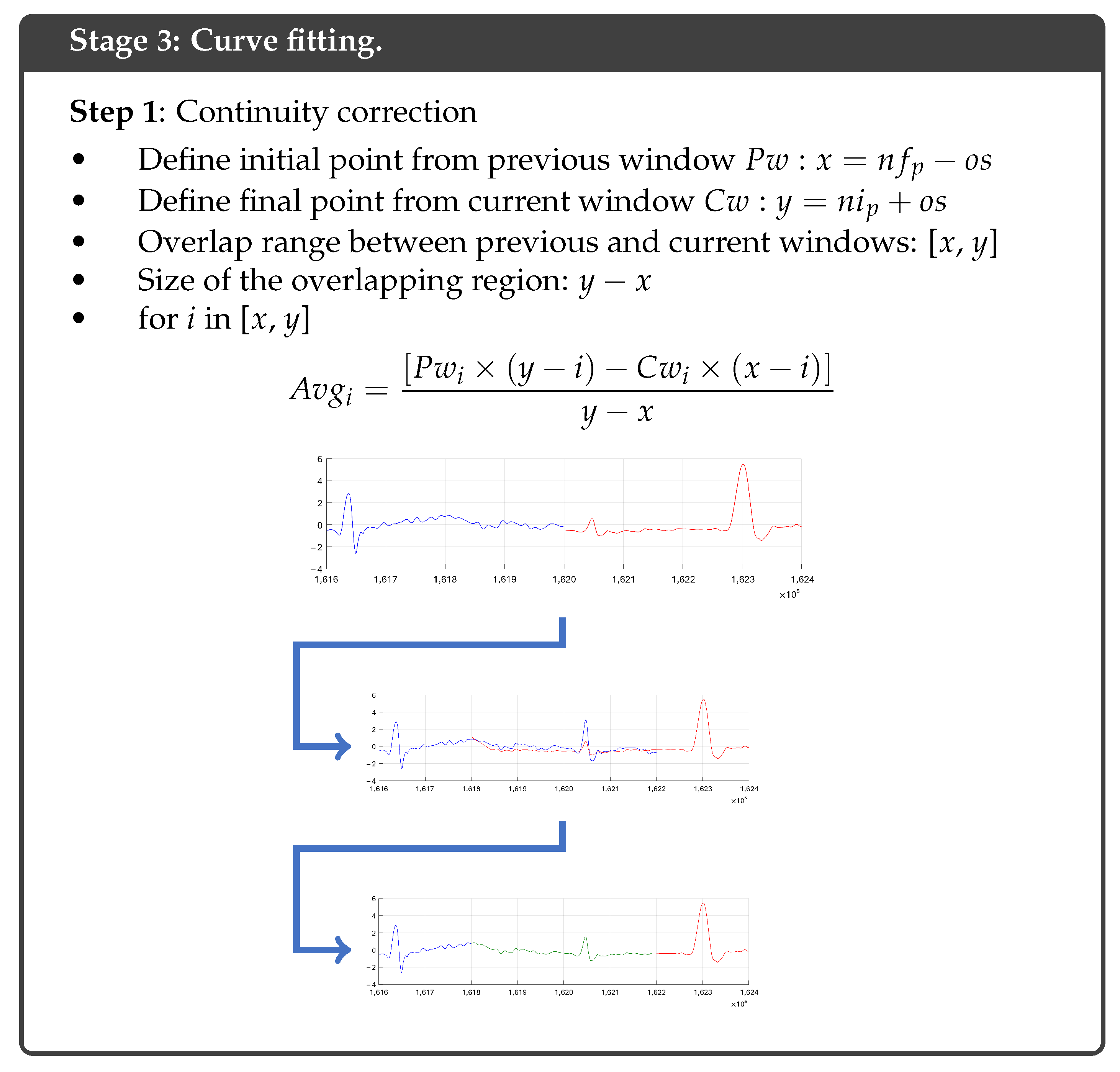
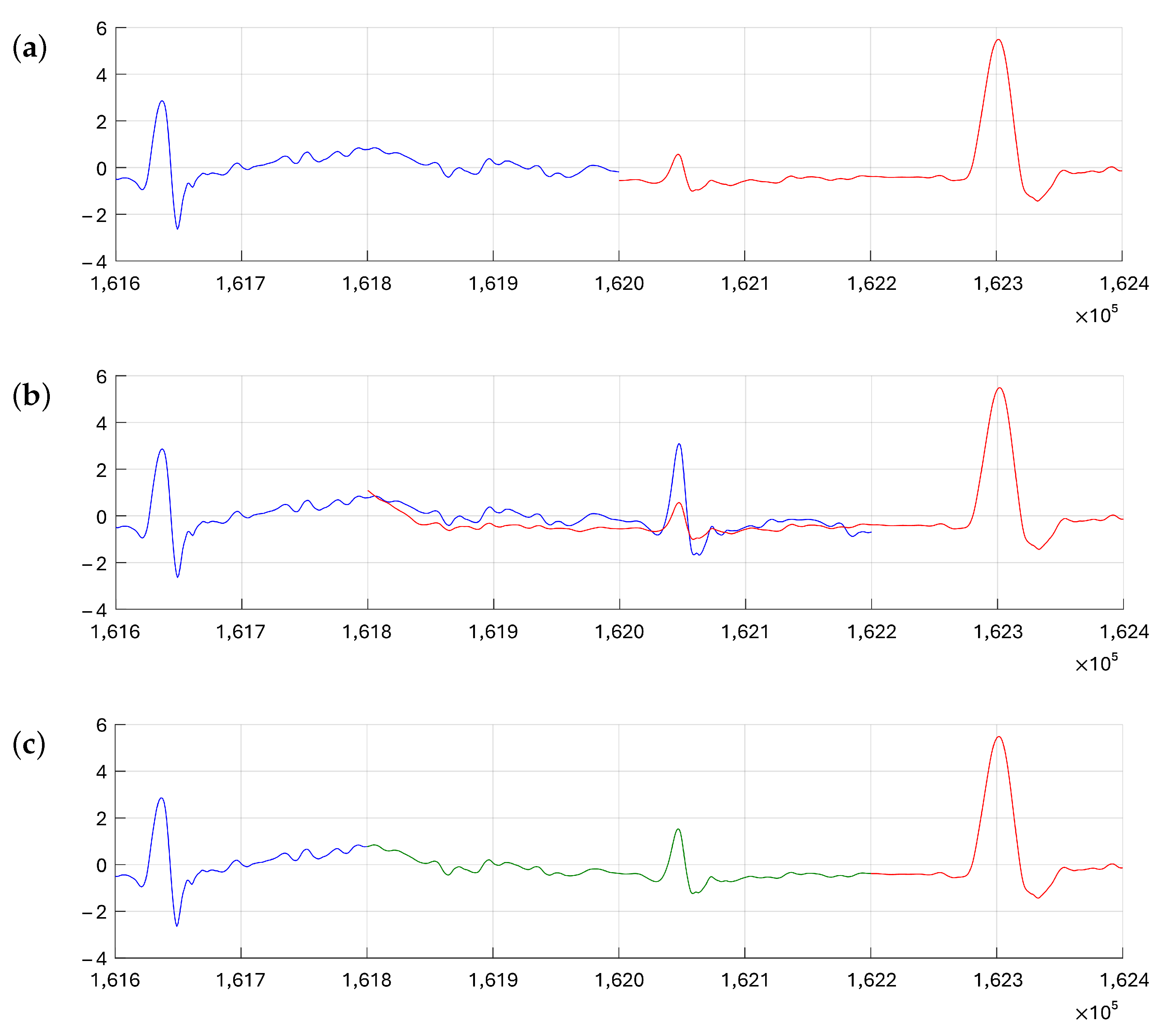
3.5. Stage 3: Curve Fitting

Due to the nature of windowed signal processing, continuity between adjacent windows is not guaranteed and there may be small offsets between them. Thus, curve fitting is the final stage of the proposed algorithm, composing a continuous signal by adjusting each of the windows that have been processed to the adjacent ones. This will result in the final record to be analyzed through clustering. A schematic of this stage is shown in Figure 15. As an example, Figure 16a shows how there is a discontinuity between the resulting signals from windows 3 (in blue) and 4 (in red) of record r01 of the ADFECGDB database after the PCA analysis and polarity correction described above. To solve this, the use of the parameter $os$ as defined in Stage 1 creates an overlapping region between these two windows, as can be seen in Figure 16b. This overlapping region between adjacent windows allows to compute a weighted average (in green in Figure 16c) from the two different signals, where continuity can be enforced by making the weight of each component at each sample to be proportional to the sample position within the overlapping region. In this way, at the beginning of the overlapping region, the signal from the preceding window ($Pw$) is considered with unity weight, which decreases to zero at the end of the region; on the other hand, the weight from the component from the following window ($Cw$) moves from zero, at the beginning of the overlapping region, to one at the end of that region.

Concretely, and using the notation introduced in Figure 6, the overlapping region is defined by its initial, x, and final, y, sample positions:

$$\begin{array}{c}x=n{f}_p-os\end{array}$$

(7)

$$\begin{array}{c}y=n{i}_c+os\end{array}$$

(8)

where $n{i}_c$ is the initial sample of the current window ($Cw$) and $n{f}_p$ is the final sample of the previous window ($Pw$). With this, the curve fitting procedure is computed as a weighted average in the [x,y] range. Thus, the i-th sample of this weighted average, $Av{g}_i$, is computed as: 

$$Av{g}_i={\displaystyle \frac{[P{w}_i\times (y-i)-C{w}_i\times (x-i)]}{y-x}}$$

(9)

where $P{w}_i$ is the value of the component from the preceding window (in blue in Figure 16b) and $C{w}_i$ is the value of the component from the current window (in red in Figure 16b). This all is summarized in Algorithm 5.

Algorithm 5 Curve fitting.

1: Step 1: Continuity correction 2: procedure CurveFit($Pw$, $Cw$, $os$) 3:     $x\leftarrow Pw:n{f}_p$ subtracting $os$ 4:     $y\leftarrow Cw:n{i}_p$ adding $os$ 5:     for $i\leftarrow x$ to y do 6:         $Master\left[i\right]\leftarrow \frac{Pw\left[i\right]\times (y-i)-Cw\left[i\right]\times (x-i)}{y-x}$ 7:     end for 8: end procedure

4. Validation and Results

As previously described, the objective of the proposed framework is to produce an aECG master signal from the PCA-based analysis above that will be fed to the clustering algorithm proposed in [14]. It is important to note that in [14] a study to establish the optimal value of the number of samples in the data window for the clustering classification was carried out. This study indicated that, in general, there was no noticeable difference in the effectiveness of the classification results for windows from 10,000 to 60,000 samples. Thus, 50,000- and 60,000-sample windows were selected in [14] for PhysioNet’s ADFECGDB [50] records and for PhysioNet’s Challenge 2013 Training Set A [53] records, respectively. In this work, a new study has been carried out in order to determine the optimal value of the number of samples in the data window for the PCA-based analysis described above and for the clustering-based fHR extraction, considering different $ws$ values for each method. For this study, PhysioNet’s ADFECGDB records have been used to train the algorithm and to derive the optimum parameter values, while the Challenge 2013 Training Set A has been used as a test and validation database with these parameters determined during the training phase. This will be described in the following subsections after defining the metrics used to evaluate the performance of the proposed framework.

4.1. Performance Metrics

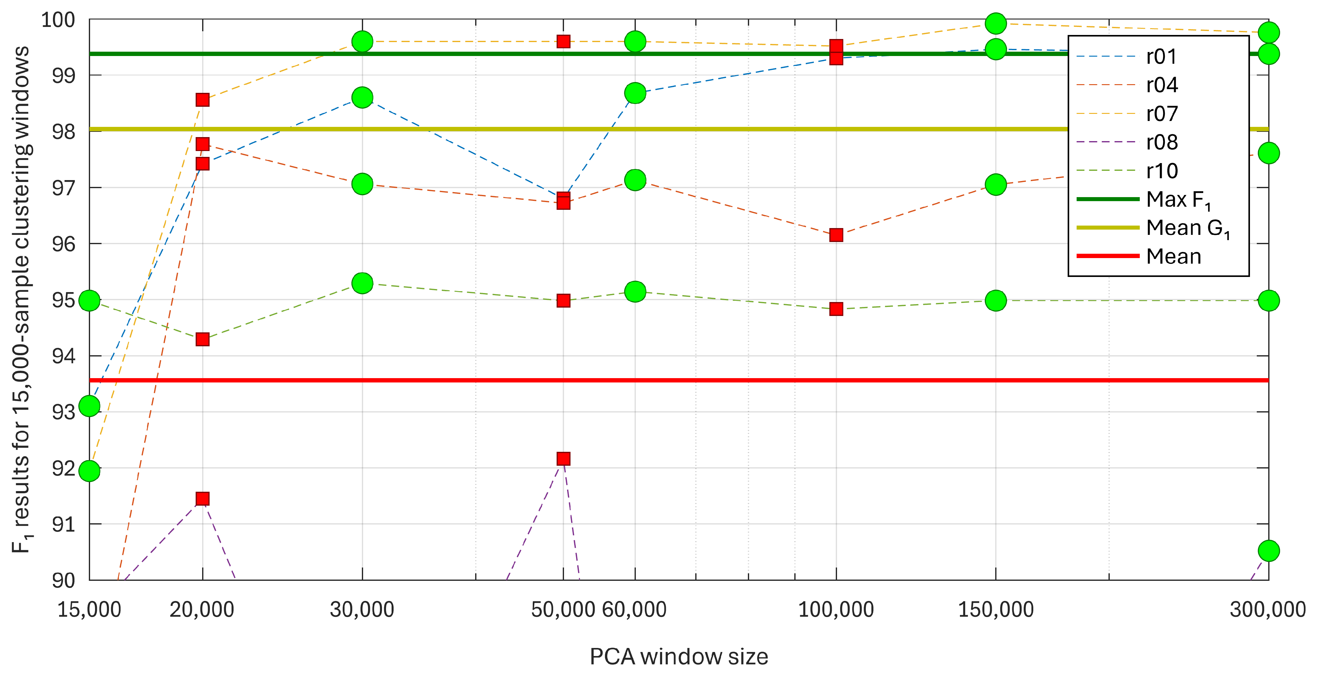
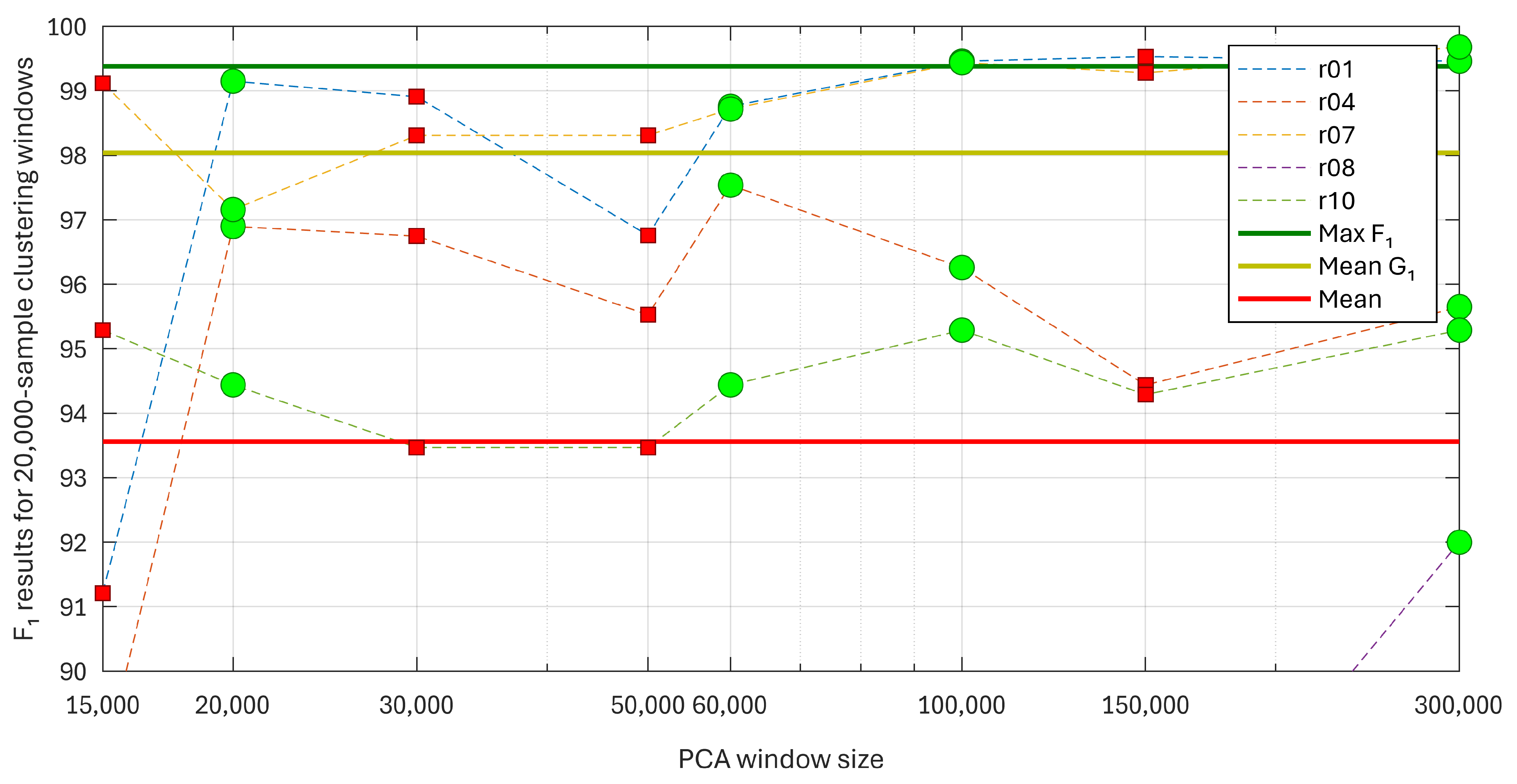
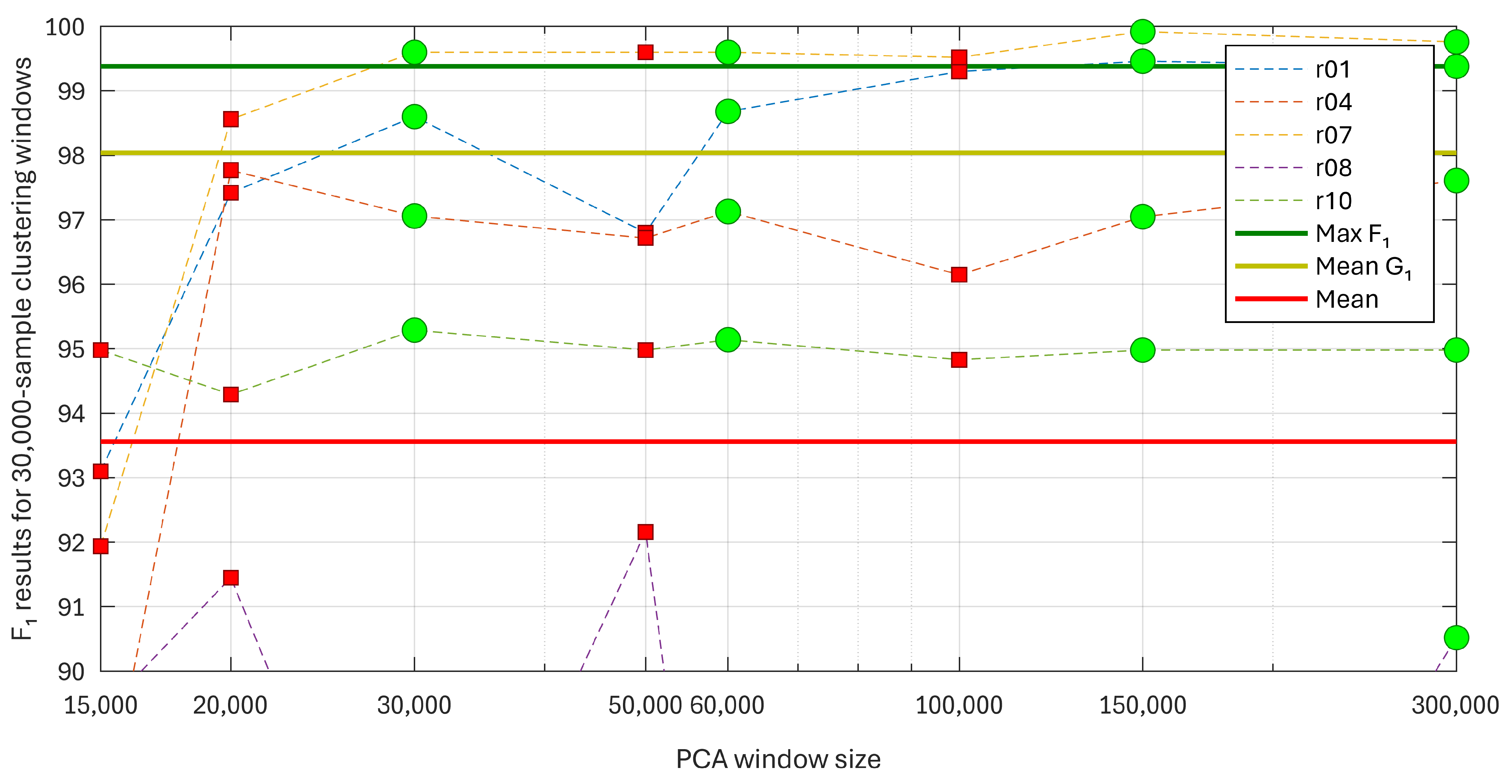
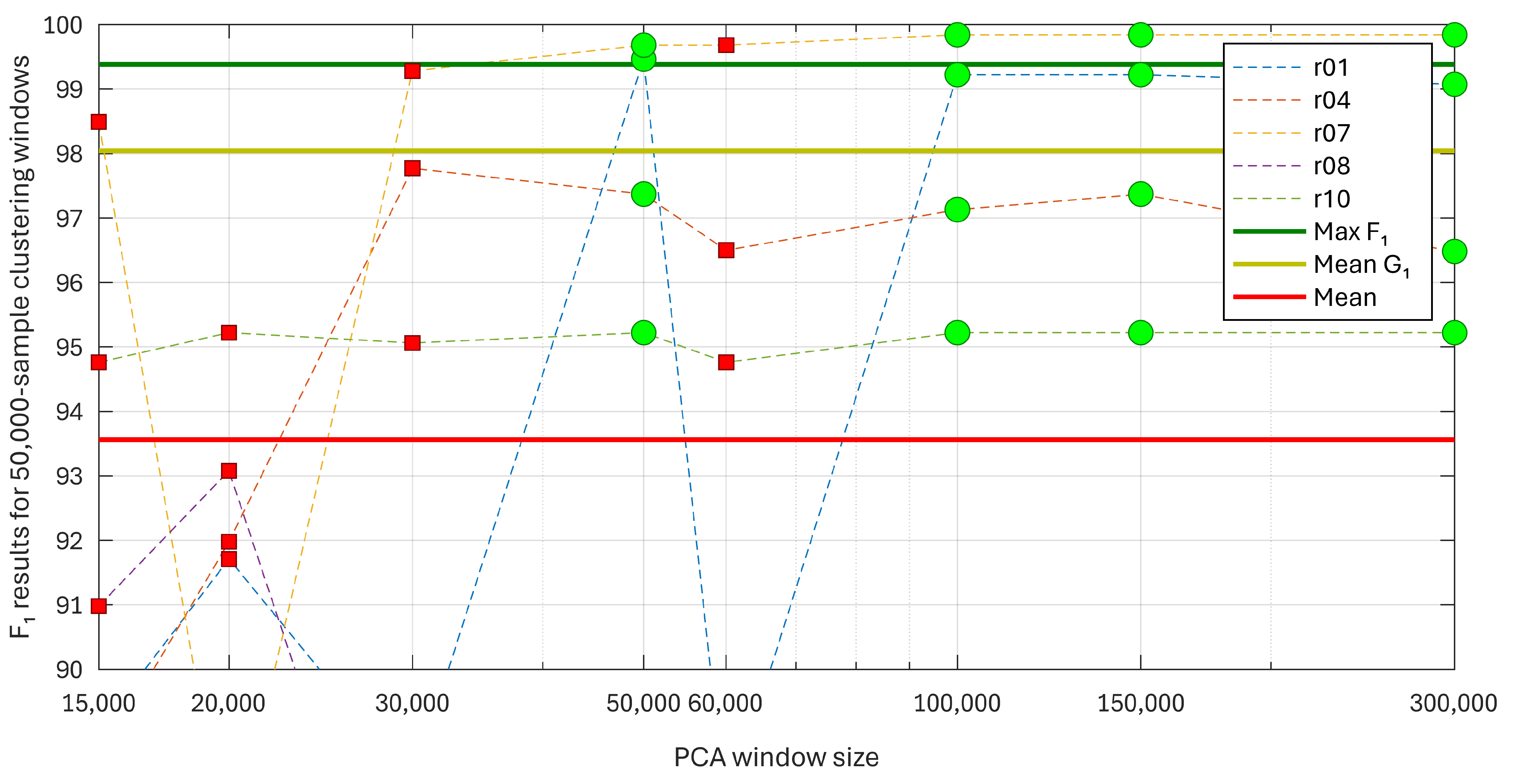
In [14] the different records were evaluated through the analysis of individual channels, discarding those presenting artifacts and/or noisy fragments, since these provided poor results. For the evaluation of results [14], values such as sensitivity ($Se$), positive diagnostic value ($PPV$), accuracy ($Acc$), and $F_1$ [24] were used:

$$\begin{array}{c}Se={\displaystyle \frac{TD}{TD+FN}}\end{array}$$

(10)

$$\begin{array}{c}PPV={\displaystyle \frac{TD}{TD+FP}}\end{array}$$

(11)

$$\begin{array}{c}{F}_1=2\times {\displaystyle \frac{PPV\times Se}{PPV+Se}}\end{array}$$

(12)

where:

$$F_1={\displaystyle \frac{2\times TD}{2\times TD+FN+FP}}.$$

(13)

In these equations, $TD$ represents true-detected fetal QRS complexes, and $FP$ and $FN$ are false negatives and false positives, respectively [14]. In the following, $F_1$ will be used as the control and comparison parameter.

4.2. Training

The algorithm in [14] was trained using PhysioNet’s ADFECGDB records, which include fetal R-wave markers that allow the calculation of different accuracy and performance parameters. For the training of this algorithm [14], the different recordings were used as a training set to establish the thresholds separating the different min-max scenarios for the signal, the optimal value of the data window size for the clustering classification, the number of times to repeat clustering using the new initial cluster medoid positions, and some other parameters. The results were classified into two groups, where group 1 included the records that a specialist doctor had previously selected and that were visually suitable for analysis. Group 2 included records with noisy fragments or artifacts, which led to a less efficient clustering-based identification of fetal heartbeats.

As described above, the presented algorithm has been also trained using the five ADFECGBD database records, obtaining satisfactory results without the need to select suitable channels since a single aECG master channel resulting from the PCA analysis was fed to the clustering-based fHR monitor. In order to evaluate this approach in comparison to the analysis in [14], three control values have been considered for the $F_1$ results: the first one is the maximum value of $F_1$ ($Max\_F_1$) obtained in any of the channels of the register evaluated in [14], the second one is the average value of the $F_1$ data obtained from all channels in group 1 ($Mean\_Grou{p}_1$), and the third control value is the average $F_1$ from all channels in both group 1 and group 2 ($Mean\_F_1$). All of these values were calculated using an analysis window of 50,000 samples in [14]. The results provided by the proposed algorithm and their respective comparison to the results in [14] are presented in

Table 1. Results of clustering for fHR monitoring with clustering windows of 15,000 samples (results in italics indicate when the PCA $ws$ is a multiple of the clustering window size, results in bold correspond to the best results for each record, grey box highlights coincident window sizes for both PCA and clustering).

		ADFECGDB Record
		r01	r04	r07	r08	r10
	PCA $\mathit{ws}$	${\mathit{F}}_{\mathbf{1}}$ (%)	${\mathit{F}}_{\mathbf{1}}$ (%)	${\mathit{F}}_{\mathbf{1}}$ (%)	${\mathit{F}}_{\mathbf{1}}$ (%)	${\mathit{F}}_{\mathbf{1}}$ (%)
Training results derived from the proposed framework	15,000	93.10	87.4	91.94	89.35	94.98
	20,000	97.42	97.77	98.56	91.45	94.29
	30,000	98.60	97.06	99.60	84.52	95.29
	50,000	96.8	96.72	99.60	92.16	94.98
	60,000	98.68	97.13	99.60	82.59	95.14
	100,000	99.3	96.15	99.52	89.39	94.83
	150,000	99.46	97.05	99.92	82.76	94.98
	300,000	99.38	97.61	99.76	90.52	94.98
Result summary from [14]	$Max\_F_1$	99.38	97.62	98.96	99.08	98.09
	$Mean\_Grou{p}_1$	98.91	97.41	97.99	97.86	98.02
	$Mean\_F_1$	93.39	95.19	97.99	89.72	95.95
	Discarded channels	–	1	1	–	3
	Noisy channels	2, 3	3	–	2, 3	4

,

Table 2. Results of clustering for fHR monitoring with clustering windows of 20,000 samples (results in italics indicate when the PCA $ws$ is a multiple of the clustering window size, results in bold correspond to the best results for each record, grey box highlights coincident window sizes for both PCA and clustering).

		ADFECGDB Record
		r01	r04	r07	r08	r10
	PCA $\mathit{ws}$	${\mathit{F}}_{\mathbf{1}}$ (%)	${\mathit{F}}_{\mathbf{1}}$ (%)	${\mathit{F}}_{\mathbf{1}}$ (%)	${\mathit{F}}_{\mathbf{1}}$ (%)	${\mathit{F}}_{\mathbf{1}}$ (%)
Training results derived from the proposed framework	15,000	91.21	88.49	99.12	88.45	95.29
	20,000	99.15	96.90	97.16	82.39	94.44
	30,000	98.91	96.75	98.31	78.14	93.47
	50,000	96.76	95.53	98.31	85.16	93.47
	60,000	98.76	97.54	98.72	84.99	94.44
	100,000	99.46	96.26	99.44	88.68	95.29
	150,000	99.53	94.44	99.28	86.15	94.29
	300,000	99.46	95.65	99.68	92	95.29
Result summary from [14]	$Max\_F_1$	99.38	97.62	98.96	99.08	98.09
	$Mean\_Grou{p}_1$	98.91	97.41	97.99	97.86	98.02
	$Mean\_F_1$	93.39	95.19	97.99	89.72	95.95
	Discarded channels	–	1	1	–	3
	Noisy channels	2, 3	3	–	2, 3	4

,

Table 3. Results of clustering for fHR monitoring with clustering windows of 30,000 samples (results in italics indicate when the PCA $ws$ is a multiple of the clustering window size, results in bold correspond to the best results for each record, grey box highlights coincident window sizes for both PCA and clustering).

		ADFECGDB Record
		r01	r04	r07	r08	r10
	PCA $\mathit{ws}$	${\mathit{F}}_{\mathbf{1}}$ (%)	${\mathit{F}}_{\mathbf{1}}$ (%)	${\mathit{F}}_{\mathbf{1}}$ (%)	${\mathit{F}}_{\mathbf{1}}$ (%)	${\mathit{F}}_{\mathbf{1}}$ (%)
Training results derived from the proposed framework	15,000	93.10	87.40	91.94	89.35	94.98
	20,000	97.42	97.77	98.56	91.45	94.29
	30,000	98.6	97.06	99.60	84.52	95.29
	50,000	96.80	96.72	99.6	92.16	94.98
	60,000	98.68	97.13	99.6	82.59	95.14
	100,000	99.30	96.15	99.52	89.39	94.83
	150,000	99.46	97.05	99.92	82.76	94.98
	300,000	99.38	97.61	99.76	90.52	94.98
Result summary from [14]	$Max\_F_1$	99.38	97.62	98.96	99.08	98.09
	$Mean\_Grou{p}_1$	98.91	97.41	97.99	97.86	98.02
	$Mean\_F_1$	93.39	95.19	97.99	89.72	95.95
	Discarded channels	–	1	1	–	3
	Noisy channels	2, 3	3	–	2, 3	4

,

Table 4. Results of clustering for fHR monitoring with clustering windows of 50,000 samples (results in italics indicate when the PCA $ws$ is a multiple of the clustering window size, results in bold correspond to the best results for each record, grey box highlights coincident window sizes for both PCA and clustering).

		ADFECGDB Record
		r01	r04	r07	r08	r10
	PCA $\mathit{ws}$	${\mathit{F}}_{\mathbf{1}}$ (%)	${\mathit{F}}_{\mathbf{1}}$ (%)	${\mathit{F}}_{\mathbf{1}}$ (%)	${\mathit{F}}_{\mathbf{1}}$ (%)	${\mathit{F}}_{\mathbf{1}}$ (%)
Training results derived from the proposed framework	15,000	89.06	88.56	98.49	90.98	94.76
	20,000	91.71	91.98	86.90	93.08	95.22
	30,000	88.25	97.77	99.28	84.54	95.06
	50,000	99.46	97.37	99.68	89.79	95.22
	60,000	87.81	96.5	99.68	86.75	94.76
	100,000	99.22	97.13	99.84	88.17	95.22
	150,000	99.22	97.37	99.84	87.01	95.22
	300,000	99.07	96.48	99.84	89.73	95.22
Result summary from [14]	$Max\_F_1$	99.38	97.62	98.96	99.08	98.09
	$Mean\_Grou{p}_1$	98.91	97.41	97.99	97.86	98.02
	$Mean\_F_1$	93.39	95.19	97.99	89.72	95.95
	Discarded channels	–	1	1	–	3
	Noisy channels	2, 3	3	–	2, 3	4

and

Table 5. Results of clustering for fHR monitoring with clustering windows of 60,000 samples (results in italics indicate when the PCA $ws$ is a multiple of the clustering window size, results in bold correspond to the best results for each record, grey box highlights coincident window sizes for both PCA and clustering).

		ADFECGDB Record
		r01	r04	r07	r08	r10
	PCA $\mathit{ws}$	${\mathit{F}}_{\mathbf{1}}$ (%)	${\mathit{F}}_{\mathbf{1}}$ (%)	${\mathit{F}}_{\mathbf{1}}$ (%)	${\mathit{F}}_{\mathbf{1}}$ (%)	${\mathit{F}}_{\mathbf{1}}$ (%)
Training results derived from the proposed framework	15,000	93.10	87.4	91.94	89.35	94.98
	20,000	97.42	97.77	98.56	91.45	94.29
	30,000	98.60	97.06	99.60	84.52	95.29
	50,000	96.8	96.72	99.60	92.16	94.98
	60,000	98.68	97.13	99.60	82.59	95.14
	100,000	99.3	96.15	99.52	89.39	94.83
	150,000	99.46	97.05	99.92	82.76	94.98
	300,000	99.38	97.61	99.76	90.52	94.98
Result summary from [14]	$Max\_F_1$	99.38	97.62	98.96	99.08	98.09
	$Mean\_Grou{p}_1$	98.91	97.41	97.99	97.86	98.02
	$Mean\_F_1$	93.39	95.19	97.99	89.72	95.95
	Discarded channels	–	1	1	–	3
	Noisy channels	2, 3	3	–	2, 3	4

and in Figure 17, Figure 18, Figure 19, Figure 20 and Figure 21 for different clustering windows sizes. Concretely, Table 1 and Figure 17 show data with 15,000-sample windows for clustering, Table 2 and Figure 18 correspond to 20,000-sample windows, Table 3 and Figure 19 show data for 30,000-sample windows, Table 4 and Figure 20 correspond to 50,000-sample windows and, finally, Table 5 and Figure 21 show data for 60,000-sample windows. To differentiate values and understand them, italics are used in these tables to highlight when the $ws$ values used in the PCA analysis are multiples of the $ws$ used in the clustering classification, the grey box is used to highlight when the $ws$ of the PCA and the clustering classification are the same, and the bold typeface is used to highlight the best $F_1$ values. On the other hand, the last two rows of these tables show the discarded channels and noisy channels in [14]. Furthermore, the values of $Max\_F_1$, $Mean\_Grou{p}_1$, and $Mean\_F_1$ used in the Figures correspond to the maximum value of all the $Max\_F_1$ results, the average value of all the $Mean\_Grou{p}_1$ values, and the minimum value of all the $Mean\_F_1$ results that were obtained in [14], respectively. Finally, the green dots in the Figures indicate when the PCA $ws$ is a multiple of the clustering window size in the analysis and the red squares mark when they are not multiples.

It is evident from the plots in Figure 17, Figure 18, Figure 19, Figure 20 and Figure 21 how the results of $F_1$ are better when the PCA $ws$ is a multiple of the clustering window size, and $F_1$ improves with larger values of the PCA $ws$. A closer inspection of all the data resulting from the analysis presented above allows us to draw some interesting conclusions. First, results in [14] for most recordings required to discard at least one of the channels not suitable for classification, while the presented framework has proved itself to be able to generate a master aECG signal suitable for clustering classification. In the case of record r08, which includes channels seriously affected by noise and artifacts, the presented results are compromised but still produce an acceptable classification. It is also interesting to note the fact that having a PCA $ws$ that is a multiple of the window size for clustering leads to improvements in the classification and detection of fetal QRS, which will be used for testing and validation. Finally, the presented framework makes it possible to, in general, obtain optimum results with clustering window sizes over 30,000 samples, which is a reduction of the optimal clustering window size presented in [14].

4.3. Testing and Validation

The Challenge 2013 Training Set A was used to test the performance of the proposed algorithm, which makes it possible to establish a direct comparison to the results obtained in [14] for this database. As was the case for the training database, no previous medical analysis was performed to select the best records from this testing database, and a single aECG master signal was derived from each recording through the presented PCA-based algorithm. In [14] only 64 channels from 26 different recordings, preselected by a cardiology specialist, were used to test the clustering classification, while the Challenge 2013 Training Set A includes 75 records. In this way, the proposed PCA-based framework has been used to generate a single master aECG record from different recordings in the Challenge 2013 Training Set A, which has been then fed to the clustering classification in [14].

Table 6. fHR monitoring results in terms of $F_1$ for Challenge 2013 Training Set A recordings for different PCA and clustering window sizes (best $F_1$ values with the proposed PCA-based framework are shown in bold, PCA-based results underperforming beyond a 3% difference when compared to [14] are shown in italics).

	[14] (60,000-Sample Window)			PCA 15,000	PCA 30,000		PCA 60,000
Record	Used Channels	Max ${\mathit{F}}_{\mathbf{1}}$ (%)	Min ${\mathit{F}}_{\mathbf{1}}$ (%)	Cluster 15,000 ${\mathit{F}}_{\mathbf{1}}$ (%)	Cluster 15,000 ${\mathit{F}}_{\mathbf{1}}$ (%)	Cluster 30,000 ${\mathit{F}}_{\mathbf{1}}$ (%)	Cluster 15,000 ${\mathit{F}}_{\mathbf{1}}$ (%)	Cluster 20,000 ${\mathit{F}}_{\mathbf{1}}$ (%)	Cluster 30,000 ${\mathit{F}}_{\mathbf{1}}$ (%)	Cluster 60,000 ${\mathit{F}}_{\mathbf{1}}$ (%)
a03	1, 2, 4	100.00	96.88	96.47	96.47	96.47	96.47	96.47	96.47	94.94
a04	1, 3, 4	99.22	96.88	96.85	99.23	99.23	99.23	99.23	99.23	99.23
a05	1, 3, 4	100.00	97.04	99.61	100.00	100.00	100.00	100.00	100.00	100.00
a08	3, 4	100.00	99.21	72.17	80.87	99.22	82.55	97.64	96.06	98.43
a12	1, 2	99.64	99.64	99.28	99.28	99.28	99.28	99.28	99.28	99.28
a13	2, 3, 4	100.00	97.56	99.21	100.00	100.00	100.00	100.00	100.00	100.00
a14	1	97.94	97.94	90.98	91.80	96.33	90.98	85.94	96.33	97.14
a20	2, 3	100.00	96.85	100.00	100.00	100.00	100.00	99.62	100.00	100.00
a22	1, 4	100.00	100.00	86.34	96.03	96.41	96.41	96.41	96.41	96.41
a23	2, 3, 4	98.80	97.58	100.00	100.00	100.00	100.00	100.00	100.00	100.00
a24	2, 3, 4	100.00	98.36	99.18	100.00	100.00	100.00	100.00	100.00	100.00
a25	2	100.00	100.00	98.39	98.79	98.79	98.79	100.00	98.79	98.79
a28	1, 2, 3	98.16	96.95	96.97	96.97	96.97	96.97	96.95	96.05	96.64
a35	1, 2, 3, 4	98.47	97.83	97.23	97.23	97.53	97.23	97.23	97.23	97.53
a36	1, 2, 3, 4	100.00	98.49	98.20	98.20	99.10	98.20	97.89	99.10	99.40
a44	1, 2, 3, 4	100.00	97.52	99.08	99.08	99.39	99.08	99.08	99.39	99.39
a49	1, 2, 3	100.00	98.98	95.50	100.00	100.00	100.00	100.00	100.00	100.00
a55	2, 3	96.43	92.75	40.64	40.64	38.46	40.64	38.25	38.46	38.46
a61	2, 4	97.42	95.34	10.11	11.15	15.69	16.33	14.67	14.48	18.79
a62	2, 3, 4	99.30	97.18	92.96	83.75	83.75	98.26	98.26	98.26	97.20
a65	2, 4	97.87	92.53	94.29	94.29	82.68	94.29	78.23	83.27	83.27
a66	3	94.44	94.44	90.69	91.50	92.31	90.16	92.31	90.08	90.08
a67	4	91.53	91.53	87.41	84.13	87.37	85.09	92.67	87.68	91.29
a69	1	94.44	94.44	80.99	70.92	75.45	58.52	66.42	60.97	62.31
a70	1, 2	98.21	91.37	93.82	96.77	91.11	97.86	85.16	86.92	78.19
a72	1, 2, 3, 4	100.00	97.58	98.80	98.80	99.70	98.80	98.80	99.70	98.80
a15	–	–	–	66.37	65.70	58.54	73.64	80.69	94.25	93.44
a17	–	–	–	68.18	54.55	92.61	95.75	96.15	96.15	96.15
a19	–	–	–	99.21	98.81	99.21	99.21	97.62	99.21	99.21
a33	–	–	–	93.33	95.41	95.71	94.66	94.66	95.71	94.66
a37	–	–	–	95.71	96.45	96.06	98.23	97.16	97.86	96.77
a53	–	–	–	71.28	76.09	94.95	78.62	79.87	91.58	92.93
a58	–	–	–	84.06	83.10	94.96	84.21	72.92	95.68	96.03

shows the classification results, in terms of $F_1$, provided by the presented algorithm for different values of the PCA $ws$ parameter and different clustering window sizes, so $ws$ is always a multiple of the clustering window size as concluded from the training phase. Table 6 thus includes a summary of the results in [14] for the Challenge 2013 Training Set A with the maximum and minimum $F_1$ values achieved for each record, which are compared to the $F_1$ values obtained for the different combinations of PCA and clustering window sizes in the presented proposal. It must be noted that the results in [14] were obtained with a single 60,000-sample clustering window. The analysis of Table 6 allows us to conclude that, when the PCA $ws$ is larger than the clustering window, results are usually better. However, larger windows increase the computational cost and the execution time of the analysis, which is a drawback for real-time processing or any future embedded hardware implementation. In any case, these results demonstrate the benefits of the presented algorithm, since it allows us to avoid an a priori selection of channels in the recordings and to directly feed the PCA-generated master aECG signal to the clustering classification. While some individual channels provided optimum results, this PCA-based master aECG signal provides a similarly optimal classification for most records and allows us to process records that had been previously discarded for classification, as shown at the bottom section of Table 6.

5. Conclusions

A procedure based on PCA analysis to obtain a single-channel master aECG record has been presented, in order to use this master aECG signal as the input to the clustering-based classification of fetal heart beats. This new procedure performs a windowed PCA-based extraction of the master aECG signal as the most prominent PCA component, followed by a correction of the polarity of each window and a curve fitting process to eliminate any discontinuities between adjacent windows. The presented PCA-based framework has been trained with the ABDFECG database, which has allowed us to conclude that the PCA $ws$ has to be a multiple of the clustering window size for optimum performance. At the same time, the use of the PCA-based framework makes it possible to reduce the size of the clustering windows and still maintain the classification performance. The analysis of the results from the Challenge 2013 Training Set A further confirms the benefits of the presented algorithm, allowing us to classify an NI-FECG recording with no need for channel selection and reducing the effects of any noise or artifacts in some of the recording’s channels. Overall, the $F_1$ resulting from the clustering analysis of the PCA-based master aECG signal is equal to or better than the results in [14] for more than a third of all analyzed channels in [14], which required a careful selection of channels to be analyzed. Additionally, the results provided by the presented method are within a 2% margin from the $F_1$ values in [14] for approximately another third of all results in [14], with no need for channel inspection or selection in this new proposal. It must be also noted that the generation of this PCA-based master aECG signal has allowed us to analyze seven additional records from the Challenge 2013 database that had to be discarded in [14]. Future use of the presented PCA-based framework is planned within an ongoing clinical study involving the acquisition of fECG recordings for a new database comprising recordings at different gestational ages and a variety of singleton pregnancies.

References

1. Jaros, R.; Martinek, R.; Kahankova, R. Non-Adaptive Methods for Fetal ECG Signal Processing: A Review and Appraisal. Sensors 2018, 18, 3648. [Google Scholar] [CrossRef] [PubMed]
2. Kahankova, R.; Martinek, R.; Jaros, R.; Behbehani, K.; Matonia, A.; Jezewski, M.; Behar, J.A. A Review of Signal Processing Techniques for Non-Invasive Fetal Electrocardiography. IEEE Rev. Biomed. Eng. 2020, 13, 51–73. [Google Scholar] [CrossRef] [PubMed]
3. Blix, E.; Maude, R.; Hals, E.; Kisa, S.; Karlsen, E.; Nohr, E.A.; Jonge, A.d.; Lindgren, H.; Downe, S.; Reinar, L.M.; et al. Intermittent auscultation fetal monitoring during labour: A systematic scoping review to identify methods, effects, and accuracy. PLoS ONE 2019, 14, e0219573. [Google Scholar] [CrossRef] [PubMed]
4. Cunningham, F.G.; Leveno, K.J.; Bloom, S.L.; Dashe, J.S.; Hoffman, B.L.; Casey, B.M.; Spong, C.Y. Intrapartum Assessment. In Williams Obstetrics, 26th ed.; McGraw-Hill Education: New York, NY, USA, 2022. [Google Scholar]
5. Vintzileos, A.M.; Nochimson, D.J.; Guzman, E.R.; Knuppel, R.A.; Lake, M.; Schifrin, B.S. Intrapartum electronic fetal heart rate monitoring versus intermittent auscultation: A meta-analysis. Obstet. Gynecol. 1995, 85, 149–155. [Google Scholar] [CrossRef] [PubMed]
6. Ibrahim, E.A.; Al Awar, S.; Balayah, Z.H.; Hadjileontiadis, L.J.; Khandoker, A.H. A Comparative Study on Fetal Heart Rates Estimated from Fetal Phonography and Cardiotocography. Front. Physiol. 2017, 8, 764. [Google Scholar] [CrossRef] [PubMed]
7. Martinek, R.; Kahankova, R.; Jaros, R.; Barnova, K.; Matonia, A.; Jezewski, M.; Czabanski, R.; Horoba, K.; Jezewski, J. Non-Invasive Fetal Electrocardiogram Extraction Based on Novel Hybrid Method for Intrapartum ST Segment Analysis. IEEE Access 2021, 9, 28608–28631. [Google Scholar] [CrossRef]
8. Zeng, R.; Lu, Y.; Long, S.; Wang, C.; Bai, J. Cardiotocography signal abnormality classification using time-frequency features and Ensemble Cost-sensitive SVM classifier. Comput. Biol. Med. 2021, 130, 104218. [Google Scholar] [CrossRef] [PubMed]
9. Vintzileos, A.M.; Antsaklis, A.; Varvarigos, I.; Papas, C.; Sofatzis, I.; Montgomery, J.T. A randomized trial of intrapartum electronic fetal heart rate monitoring versus intermittent auscultation. Obstet. Gynecol. 1993, 81, 899–907. [Google Scholar]
10. Caliskan, E.; Cakiroglu, Y.; Corakci, A.; Ozeren, S. Reduction in caesarean delivery with fetal heart rate monitoring and intermittent pulse oximetry after induction of labour with misoprostol. J. Matern.-Fetal Neonatal Med. 2009, 22, 445–451. [Google Scholar] [CrossRef]
11. Cohen, W.R.; Ommani, S.; Hassan, S.; Mirza, F.G.; Solomon, M.; Brown, R.; Schifrin, B.S.; Himsworth, J.M.; Hayes-Gill, B.R. Accuracy and reliability of fetal heart rate monitoring using maternal abdominal surface electrodes. Acta Obstet. Gynecol. Scand. 2012, 91, 1306–1313. [Google Scholar] [CrossRef]
12. Liu, B.; Thilaganathan, B.; Bhide, A. Effectiveness of ambulatory non-invasive fetal electrocardiography: Impact of maternal and fetal characteristics. Acta Obstet. Gynecol. Scand. 2023, 102, 577–584. [Google Scholar] [CrossRef] [PubMed]
13. Pardey, J.; Moulden, M.; Redman, C.W. A computer system for the numerical analysis of nonstress test. Am. J. Obstet. Gynecol. 2002, 186, 1095–1103. [Google Scholar] [CrossRef] [PubMed]
14. Castillo, E.; Morales, D.P.; García, A.; Parrilla, L.; Ruiz, V.U.; Álvarez Bermejo, J.A. A clustering-based method for single-channel fetal heart rate monitoring. PLoS ONE 2018, 13, e0199308. [Google Scholar] [CrossRef] [PubMed]
15. Mujumdar, R.; Nadar, P.; Bondre, A.P.; Kulkarni, A.; Pathak, S. Principal Component Analysis (PCA) Based Single-Channel, Non-Invasive Fetal ECG Extraction; CareNX Innovations Pvt. Ltd.: Maharashtra, India, 2019. [Google Scholar]
16. Castillo, E.; Morales, D.P.; García, A.; Martínez-Martí, F.; Parrilla, L.; Palma, A.J. Noise Suppression in ECG Signals through Efficient One-Step Wavelet Processing Techniques. J. Appl. Math. 2013, 2013, e763903. [Google Scholar] [CrossRef]
17. Lisenbee, N.; Tyndall, J.A. Fetal Heart Rate Monitoring. In Atlas of Emergency Medicine Procedures; Ganti, L., Ed.; Springer: New York, NY, USA, 2016; pp. 639–642. [Google Scholar] [CrossRef]
18. Bin Queyam, A.; Kumar Pahuja, S.; Singh, D. Quantification of Feto-Maternal Heart Rate from Abdominal ECG Signal Using Empirical Mode Decomposition for Heart Rate Variability Analysis. Technologies 2017, 5, 68. [Google Scholar] [CrossRef]
19. Barnova, K.; Martinek, R.; Jaros, R.; Kahankova, R. Hybrid Methods Based on Empirical Mode Decomposition for Non-Invasive Fetal Heart Rate Monitoring. IEEE Access 2020, 8, 51200–51218. [Google Scholar] [CrossRef]
20. Apsana, S.; Suresh, M.G.; Aneesh, R.P. A novel algorithm for early detection of fetal arrhythmia using ICA. In Proceedings of the 2017 International Conference on Intelligent Computing, Instrumentation and Control Technologies (ICICICT), Kerala, India, 6–7 July 2017; pp. 1277–1283. [Google Scholar] [CrossRef]
21. Abramowicz, J.S.; Barnett, S.B.; Duck, F.A.; Edmonds, P.D.; Hynynen, K.H.; Ziskin, M.C. Fetal Thermal Effects of Diagnostic Ultrasound. J. Ultrasound Med. 2008, 27, 541–559. [Google Scholar] [CrossRef]
22. Castillo, E.; Morales, D.P.; Botella, G.; García, A.; Parrilla, L.; Palma, A.J. Efficient wavelet-based ECG processing for single-lead FHR extraction. Digit. Signal Process. 2013, 23, 1897–1909. [Google Scholar] [CrossRef]
23. Martinek, R.; Kahankova, R.; Jezewski, J.; Jaros, R.; Mohylova, J.; Fajkus, M.; Nedoma, J.; Janku, P.; Nazeran, H. Comparative Effectiveness of ICA and PCA in Extraction of Fetal ECG From Abdominal Signals: Toward Non-invasive Fetal Monitoring. Front. Physiol. 2018, 9, 338138. [Google Scholar] [CrossRef]
24. Behar, J.; Johnson, A.; Clifford, G.D.; Oster, J. A Comparison of Single Channel Fetal ECG Extraction Methods. Ann. Biomed. Eng. 2014, 42, 1340–1353. [Google Scholar] [CrossRef]
25. Panigrahy, D.; Sahu, P.K. Extraction of fetal ECG signal by an improved method using extended Kalman smoother framework from single channel abdominal ECG signal. Australas. Phys. Eng. Sci. Med. 2017, 40, 191–207. [Google Scholar] [CrossRef] [PubMed]
26. He, P.J.; Chen, X.M.; Liang, Y.; Zeng, H.Z. Extraction for fetal ECG using single channel blind source separation algorithm based on multi-algorithm fusion. MATEC Web Conf. 2016, 44, 01026. [Google Scholar] [CrossRef]
27. Rahmati, A.; Setarehdan, S.; Araabi, B. A PCA/ICA based Fetal ECG Extraction from Mother Abdominal Recordings by Means of a Novel Data-driven Approach to Fetal ECG Quality Assessment. J. Biomed. Phys. Eng. 2017, 7, 37–50. [Google Scholar]
28. Wang, Y.; Fu, Y.; He, Z. Fetal Electrocardiogram Extraction Based on Fast ICA and Wavelet Denoising. In Proceedings of the 2018 2nd IEEE Advanced Information Management, Communicates, Electronic and Automation Control Conference (IMCEC), Xi’an, China,, 25–27 May 2018; pp. 466–469. [Google Scholar] [CrossRef]
29. Sutha, P.; Jayanthi, V. Fetal Electrocardiogram Extraction and Analysis Using Adaptive Noise Cancellation and Wavelet Transformation Techniques. J. Med. Syst. 2017, 42, 21. [Google Scholar] [CrossRef] [PubMed]
30. Zarzoso, V.; Nandi, A. Noninvasive fetal electrocardiogram extraction: Blind separation versus adaptive noise cancellation. IEEE Trans. Biomed. Eng. 2001, 48, 12–18. [Google Scholar] [CrossRef] [PubMed]
31. Zeng, Y.; Liu, S.; Zhang, J. Extraction of Fetal ECG Signal via Adaptive Noise Cancellation Approach. In Proceedings of the 2008 2nd International Conference on Bioinformatics and Biomedical Engineering, Shanghai, China, 16–18 May May 2008; pp. 2270–2273. [Google Scholar] [CrossRef]
32. Hassanpour, H.; Parsaei, A. Fetal ECG Extraction Using Wavelet Transform. In Proceedings of the 2006 International Conference on Computational Inteligence for Modelling Control and Automation and International Conference on Intelligent Agents Web Technologies and International Commerce (CIMCA’06), Sydney, NSW, Australia, 28 November–1 December 2006; p. 179. [Google Scholar] [CrossRef]
33. Wu, S.; Shen, Y.; Zhou, Z.; Lin, L.; Zeng, Y.; Gao, X. Research of fetal ECG extraction using wavelet analysis and adaptive filtering. Comput. Biol. Med. 2013, 43, 1622–1627. [Google Scholar] [CrossRef] [PubMed]
34. Morales, D.P.; García, A.; Castillo, E.; Meyer-Baese, U.; Palma, A.J. Wavelets for full reconfigurable ECG acquisition system. In Proceedings of the Independent Component Analyses, Wavelets, Neural Networks, Biosystems, and Nanoengineering IX. International Society for Optics and Photonics, Orlando, FL, USA, 25–29 April 2011; Volume 8058, p. 805817. [Google Scholar] [CrossRef]
35. Azbari, P.G.; Mohaqeqi, S.; Gashti, N.G.; Mikaili, M. Introducing a combined approach of empirical mode decomposition and PCA methods for maternal and fetal ECG signal processing. J. Matern.-Fetal Neonatal Med. 2016, 29, 3104–3109. [Google Scholar] [CrossRef] [PubMed]
36. Sameni, R.; Shamsollahi, M.; Jutten, C. Filtering Electrocardiogram Signals Using the Extended Kalman Filter. In Proceedings of the 2005 IEEE Engineering in Medicine and Biology 27th Annual Conference, Shanghai, China, 17–18 January 2005; pp. 5639–5642. [Google Scholar] [CrossRef]
37. Camps-Valls, G.; Martínez-Sober, M.; Soria-Olivas, E.; Magdalena-Benedito, R.; Calpe-Maravilla, J.; Guerrero-Martínez, J. Foetal ECG recovery using dynamic neural networks. Artif. Intell. Med. 2004, 31, 197–209. [Google Scholar] [CrossRef] [PubMed]
38. Behar, J.; Johnson, A.E.W.; Oster, J.; Clifford, G. An Echo State Neural Network for Foetal ECG Extraction Optimised by Random Search. In Proceedings of the Machine Learning for Clinical Data Analysis and Healthcare, NIPS Workshop 2013, Lake Tahoe, NV, USA, 9–10 December 2013; p. 5. [Google Scholar]
39. Fotiadou, E.; Vullings, R. Multi-Channel Fetal ECG Denoising With Deep Convolutional Neural Networks. Front. Pediatr. 2020, 8, 508. [Google Scholar] [CrossRef]
40. Meyer-Baese, U. Adaptive Systems. In Digital Signal Processing with Field Programmable Gate Arrays; Meyer-Baese, U., Ed.; Signals and Communication Technology; Springer: Berlin/Heidelberg, Germany, 2014; pp. 533–630. [Google Scholar] [CrossRef]
41. Ziani, S.; El Hassouani, Y. Fetal Electrocardiogram Analysis Based on LMS Adaptive Filtering and Complex Continuous Wavelet 1-D. In Big Data and Networks Technologies; Lecture Notes in Networks and, Systems, Farhaoui, Y., Eds.; Springer: Cham, Switzerland, 2020; pp. 360–366. [Google Scholar] [CrossRef]
42. Swarnalath, R.; Prasad, D.V. A Novel Technique for Extraction of FECG using Multi Stage Adaptive Filtering. J. Appl. Sci. 2010, 10, 319–324. [Google Scholar] [CrossRef]
43. Ramli, D.A.; Shiong, Y.H.; Hassan, N. Blind Source Separation (BSS) of Mixed Maternal and Fetal Electrocardiogram (ECG) Signal: A comparative Study. Procedia Comput. Sci. 2020, 176, 582–591. [Google Scholar] [CrossRef]
44. Madhulatha, T.S. An Overview on Clustering Methods. IOSR J. Eng. 2012, 2, 719–725. [Google Scholar] [CrossRef]
45. Clifford, G.D.; Silva, I.; Behar, J.; Moody, G.B. Noninvasive Fetal ECG analysis. Physiol. Meas. 2014, 35, 1521–1536. [Google Scholar] [CrossRef] [PubMed]
46. Țarălungă, D.; Gussi, I.; Strungaru, R. A New Method for Fetal Electrocardiogram Denoising Using Blind Source Separation and Empirical Mode Decomposition. Rev. Roum. Sci. Techn.–Électrotechn. Énerg. 2016, 61, 94–98. [Google Scholar]
47. Kanjilal, P.; Palit, S.; Saha, G. Fetal ECG extraction from single-channel maternal ECG using singular value decomposition. IEEE Trans. Biomed. Eng. 1997, 44, 51–59. [Google Scholar] [CrossRef] [PubMed]
48. Kanjilal, P.; Saha, G. Fetal ECG extraction from single channel maternal ECG using SVD and SVR spectrum. In Proceedings of the 17th International Conference of the Engineering in Medicine and Biology Society, Montreal, QC, Canada, 20–23 September 1995; Volume 1, pp. 187–188. [Google Scholar] [CrossRef]
49. Meyer-Baese, U.; Muddu, H.; Schinhaerl, S.; Kumm, M.; Zipf, P. Real-time fetal ECG system design using embedded microprocessors. In Proceedings of the Sensing and Analysis Technologies for Biomedical and Cognitive Applications 2016. International Society for Optics and Photonics, Baltimore, MD, USA, 17–21 April 2016; Volume 9871, p. 987106. [Google Scholar] [CrossRef]
50. Matonia, A.; Jezewski, J.; Kupka, T.; Horoba, K.; Wrobel, J.; Gacek, A. Abdominal and Direct Fetal ECG Database . Biomed. Eng. Tech. 2012, 57, 383–394. [Google Scholar] [CrossRef]
51. Goldberger, A.L.; Amaral, L.A.N.; Glass, L.; Hausdorff, J.M.; Ivanov, P.C.; Mark, R.G.; Mietus, J.E.; Moody, G.B.; Peng, C.K.; Stanley, H.E. PhysioBank, PhysioToolkit, and PhysioNet. Circulation 2000, 101, e215–e220. [Google Scholar] [CrossRef]
52. Open Data Commons Public Domain Dedication and License (PDDL) v1.0—Open Data Commons: Legal Tools for Open Data. Available online: https://physionet.org/about/licenses/open-data-commons-open-database-license-v10/ (accessed on 25 March 2024).
53. Silva, I.; Behar, J.A.; Sameni, R.; Tingting, Z.; Clifford, G.; Moody, G. Noninvasive Fetal ECG—The PhysioNet Computing in Cardiology Challenge. 2013. Available online: https://physionet.org/content/challenge-2013/1.0.0/ (accessed on 25 March 2024).
Figure 1. Example of an aECG channel, composed of mECG, fECG, and different noises.
Electronics 13 01264 g001
Figure 2. Proposed processing framework.
Electronics 13 01264 g002
Figure 3. (a) Fragment of channel #1 in record r01 from ADFECGDB; (b) resulting signal after one-step wavelet-based preprocessing.
Electronics 13 01264 g003
Figure 4. Stage 1: PCA-based analysis for fetal ECG extraction.
Electronics 13 01264 g004
Figure 5. (a) Fragments of the four channels of register r04 from ADFECGDB, corresponding to the third window to be analyzed. The 4000 samples in w s are shown in blue, with the two overlap fragments shown in red ( o s is 1000 samples). (b) Master aECG channel derived from the PCA analysis.
Electronics 13 01264 g005
Figure 6. Complete signal fragmented into windows, which are increased in size (in red) with the overlap fragments.
Electronics 13 01264 g006
Figure 7. (a) Fragments from aECG channels in the denoised r04 record; (b) Master aECG channel derived from the PCA analysis.
Electronics 13 01264 g007
Figure 8. Stage 2: Polarization check.
Electronics 13 01264 g008
Figure 9. Distances for scenario analysis of a QRS complex: (a) non-inverted QRS-complex, (b) inverted QRS-complex.
Electronics 13 01264 g009
Figure 10. First scenario, the first local maximum found is the P-wave (green dots correspond to j-th iteration, yellow and red dots represent ( j 1 ) -th and ( j + 1 ) -th groups, respectively).
Electronics 13 01264 g010
Figure 11. Second scenario, the first local maximum found is the R-wave (green dots correspond to j-th iteration, yellow and red dots represent ( j 1 ) -th and ( j + 1 ) -th groups, respectively).
Electronics 13 01264 g011
Figure 12. First inverted scenario, the first local maximum found is the Q-wave (green dots correspond to j-th iteration, yellow and red dots represent ( j 1 ) -th and ( j + 1 ) -th groups, respectively).
Electronics 13 01264 g012
Figure 13. Second inverted scenario, the first local maximum found is the S-wave (green dots correspond to j-th iteration, yellow and red dots represent ( j 1 ) -th and ( j + 1 ) -th groups, respectively).
Electronics 13 01264 g013
Figure 14. QRS polarization correction: (a) fragment of the PCA-derived aECG master signal from r01 record with wrong polarity (red triangles mark R-peaks); (b) resulting fragment after polarity correction (blue triangles mark R-peaks).
Electronics 13 01264 g014
Figure 15. Stage 3: Curve fitting.
Electronics 13 01264 g015
Figure 16. (a) Discontinuity between preceding window ( P w , in blue) and current window ( C w , in red) without overlap; (b) overlapping region between P w (in blue) and C w (in red) defined by o s ; and (c) curve fitting (in green) between P w (in blue) and C w (in red).
Electronics 13 01264 g016
Figure 17. Plot of F 1 training results for ADFECGDB with clustering windows of 15,000 samples (green dots correspond to PCA w s that are multiples of the clustering window size).
Electronics 13 01264 g017
Figure 18. Plot of F 1 training results for ADFECGDB with clustering window of 20,000 samples (green dots correspond to PCA w s that are multiples of the clustering window size).
Electronics 13 01264 g018
Figure 19. Plot of F 1 training results for ADFECGDB with clustering window of 30,000 samples (green dots correspond to PCA w s that are multiples of the clustering window size).
Electronics 13 01264 g019
Figure 20. Plot of F 1 training results for ADFECGDB with clustering window of 50,000 samples (green dots correspond to PCA w s that are multiples of the clustering window size).
Electronics 13 01264 g020
Figure 21. Plot of F 1 training results for ADFECGDB with clustering window of 60,000 samples (green dots correspond to PCA w s that are multiples of the clustering window size).
Electronics 13 01264 g021