Controllable Spatial Filtering Method in Lensless Imaging

Abstract

We propose a method for multiple-depth extraction in diffraction grating imaging. A diffraction grating can optically generate a diffraction image array (DIA) having parallax information about a three-dimensional (3D) object. The optically generated DIA has the characteristic of forming images periodically, and the period depends on the depth of the object, the wavelength of the light source, and the grating period of the diffraction grating. The depth image can be extracted through the convolution of the DIA and the periodic delta function array. Among the methods for extracting depth images through the convolution characteristics of a parallax image array (PIA) and delta function array, an advanced spatial filtering method for the controllable extract of multiple depths (CEMD) has been studied as one of the reconstruction methods. And that possibility was confirmed through a lens-array-based computational simulation. In this paper, we aim to perform multiple-depth extraction by applying the CEMD method to a DIA obtained optically through a diffraction grating. To demonstrate the application of the CEMD in diffraction grating imaging, a theoretical analysis is performed to apply the CEMD in diffraction grating imaging; the DIA is acquired optically, and the spatial filtering process is performed through computational methods and then compared with the conventional single-depth extraction method in diffraction grating imaging. The application of the CEMD to DIA enables the simultaneous reconstruction of images corresponding to multiple depths through a single spatial filtering process. To the best of our knowledge, this is the first research on the extraction of multiple-depth images in diffraction grating imaging.

1. Introduction

In the field of three-dimensional (3D) display and processing, a parallax image array (PIA) stands out as an exceptionally efficient format, encapsulating full parallax information of a 3D object. 3D imaging technologies that can acquire 3D scenes include integral imaging [1,2,3,4,5,6], light field imaging [7,8,9,10,11,12], and lensless imaging [13,14,15,16,17]. Among these imaging methods, both integral imaging and light field imaging are characterized by acquisition systems comprising arrays of individual imaging optical elements such as lenses and cameras [18,19,20,21,22,23,24]. In contrast, diffraction grating imaging, one of the lensless 3D imaging methods, presents a unique approach [13,14]. Utilizing a single optical element, it has the inherent capability to generate parallax images (PIs), showcasing the efficiency and simplicity of its optics in comparison to systems relying on arrays of lenses and cameras. These differences in acquisition systems lead to distinctions in the reconstruction process of the 3D scene. In imaging systems featuring an array of optical elements, the allocation of space for a single parallax image (PI) within the PIA is dictated by the field of view of each optical element. Consequently, the predominant approach for reconstructing the three-dimensional scene in such configurations is the utilization of the back projection method. Contrastingly, in diffraction grating imaging, the generation of a PIA is via a solitary optical element, posing challenges in precisely defining the area occupied by an individual PI. Consequently, the reconstruction of a 3D scene in diffraction grating imaging adopts a distinctive approach, relying on the convolution operation between the PIA and a delta function array. This method allows for 3D scene reconstruction, taking into account the unique properties of diffraction grating imaging, which generates a PIA by a single optical element.

A PIA has a unique characteristic in which individual PIs within the PIA are formed periodically in the imaging space by dynamically responding to changes in the depth of the object. This periodicity becomes particularly pronounced when subjected to the convolution operation with a delta function array; accentuation occurs when the periods align, while a distinctive reduction is observed when the periods diverge. Therefore, leveraging this characteristic, the reconstruction of an image corresponding to a specific depth is made possible through the judicious application of the sifting property intrinsic to the convolution between periodic functions (SCPF). The spatial filtering method using SCPF can be universally applied to all 3D imaging systems wherein there exists a correspondence between the spatial period of the PIA and the depth of the object.

Various spatial filtering methods have been researched for enhancing the scaling, depth resolution, and image resolution of reconstructed images, using the principles of SCPF [13,14,25]. Within the methods of applying SCPF, research on an advanced spatial filtering technique, namely the controllable extraction of multiple depths (CEMD), has emerged as a notable way for image reconstruction. The viability of this method was substantiated through experimentation, utilizing a PIA generated via computational integral imaging simulation, employing a lens array model rather than an actual optical system [25]. Nevertheless, this study has limitations because it was conducted only through simulations with optimized optical conditions, excluding various optical factors such as aberration that can affect the resolution and spatial period of a PIA. Additionally, the PIA is not obtained through real optical systems, so verification of the realism and practical applicability of the results is required.

Note that just as a PIA is called an element image array (EIA) in integral imaging, in diffraction grating imaging it is called a diffraction image array (DIA), and an individual PI within the DIA are called diffraction images (DIs).

In this paper, we employ the CEMD to diffraction grating imaging, aiming to demonstrate its practical applicability within real-world optical systems. To verify that it can be implemented in diffraction grating imaging, DIs are generated and acquired through optical methods. To apply the CEMD to a diffraction grating imaging system, we conduct a theoretical analysis of geometric optical relationships. This includes considerations of the spatial coordinates of the DI, taking into account the wavelength of the light source and the grating period of the diffraction grating. Additionally, we examine the spatial period of the PIA, corresponding to the depth of the object. A wave optical analysis is performed to explain the imaging formation of the PIA generated by the diffraction grating. For this purpose, the relevant intensity impulse response, scaled object intensity, and intensity of the DIA are derived. We then derive a mathematical expression for the CEMD in diffraction grating imaging. We perform experiments to simultaneously extract controllable depth images corresponding to multiple depths in a single spatial filtering process and validate its applicability to diffraction grating imaging systems.

2. Basic Theory in Diffraction Grating Imaging

2.1. Geometric Relations

In diffraction grating imaging, incident light that is scattered from an object and enters a diffraction grating placed along the optical path is diffracted as it encounters the diffraction grating. This diffraction grating plays a pivotal role in diffracting incident light into multiple rays and coordinating their formation into a distinct optical phenomenon known as the DIA. The DIA, characterized by its unique parallax perspectives, is imaged in complex response to the varying depths of objects, wavelengths of light sources, and grating periods. The DIA may be captured by an image-acquisition device such as a camera. In this process, the depth information inherent in the 3D object space is converted to two-dimensional (2D) spatial period information within the DIA. The spatially periodic arrangement within the DIA is correlated with the depth variation present in the object space. The spatial period of the DIA undergoes a reduction as the depth of the object decreases, conversely expanding as the depth of the object increases. The imaging depth and size of the DIs generated by the diffraction grating imaging are identical to the depth and size of the object. These characteristics set it apart from 3D imaging methods relying on a lens array.

Figure 1a illustrates the 2D geometric arrangement involving a point object, the DIs of the point object on the DIA plane, and the imaging points of the DIs imaged through an imaging lens in diffraction grating imaging. In this context, let us make the assumption that a point object is positioned at ($x_{D0th},z_O$). Consequently, the z-coordinates of all the diffraction images are uniformly set to $z_O$. In the configuration depicted in Figure 1a, the imaging lens is situated at a distance d from the diffraction grating. The point object situated at coordinates ($x_O,z_O$) serves as the 0th-order DI denoted as DI($x_{D0th},z_O$). By the diffraction grating in the diffraction grating imaging system, the generation of the -1st- and 1st-order DIs unfolds. Positioned at ($x_{D-1st},z_O$) and ($x_{D1st},z_O$), respectively, these DIs are generated through the ±1st-order diffraction processes induced by the diffraction grating. The diffraction angle $\theta$ is defined by the equation $\theta ={sin}^{-1}(m\lambda /a)$, where m signifies the diffraction order, $\lambda$ represents the wavelength of the incident light source, and a denotes the aperture width of the diffraction grating. Taking into account both the diffraction order and the object’s location, the x-coordinate $x_{Dmth}$ of a diffraction image is determined by

$$x_{Dmth}=x_O+|z_O-d|tan\left({sin}^{-1}\left(\frac{m\lambda }{a}\right)\right),$$

(1)

where the parameter m takes values of −1, 0, and 1, corresponding to the order of diffraction. The term $|z_O-d|$ represents the distance between the object and the diffraction grating. Equation (1) indicates that the location of the DIs produced by the diffraction grating exhibits periodicity, aligned with the diffraction order.

Based on the geometric relationship and Equation (1), the one-dimensional form of the spatial period of the DIA, contingent upon the object’s depth, can be expressed as $|x_{D(s)th}-x_{D(s-1)th}|$, where s takes values of 0 or 1. Hence, the spatial period, contingent on the object’s depth, is determined by

$$X_{z_O}=|z_O-d|tan\left({sin}^{-1}\left(\frac{\lambda }{a}\right)\right),$$

(2)

Equations (1) and (2) collectively highlight that $X_{zO}$, representing the distance between the DIs in the DIA, can exhibit variation contingent upon the wavelength of the light source employed in the DIA acquisition process. This fundamental equation encapsulates the relationship between the diffraction angle and the key parameters of the diffraction imaging system when the DI is imaged on the DIA plane, providing foundational insight into the periodicity of the diffraction image when light scattered from an object is diffracted by diffraction grating. Figure 1b provides an illustrative example featuring two point objects utilized for imaging within the system of diffraction grating imaging. The x-coordinates of the point objects are identical, with the depth of the objects from the diffraction grating being closer for the point objects represented in blue and farther away for the point objects depicted in red. As evident from the geometric relationship portrayed in Figure 1b, it becomes apparent that the spatial period of the PIA extends proportionally as the object’s position moves farther away from the diffraction grating. The characteristic of depth-related spatial period changes in the PIA constitutes a fundamental aspect that plays a crucial role in facilitating the spatial filtering process integral to the 3D image reconstruction in diffraction grating imaging.

2.2. Imaging Formation

The optical properties of a DIA can be aptly described by analyzing the intensity impulse response and scaled object intensity. Leveraging the periodic property inherent in a DIA, which is contingent on the object’s depth, provides valuable insights into the optical behavior of the imaging system. In conventional 2D imaging, when $x_D$ signifies the x-coordinate on the DIA plane, $h(x_D)$ denotes the intensity impulse response, while $f(x_D)$ stands for the scaled object intensity, accounting for image magnification factors. The image intensity can be determined by the convolution of $h(x_D)$ and $f(x_D)$, denoted as $g(x_D)$. For the 3D object, the image intensity is solely expressed as $g(x_D){|}_{z_O}=f(x_D){{|}_{z_O}\ast h(x_D)|}_{z_O}$, reflecting its dependence on $z_O$. This dependence arises from the object’s depth, impacting both the intensity impulse response and the object intensity. Hence, the image intensity, which varies with $z_O$, can be expressed by

$$g(x_D)=\int h(z_O,x_D)\ast f(z_O,x_D)d{z}_O,$$

(3)

taking into account the continuously distributed intensity of a 3D volume object, the image intensity $g(x_D)$ embodies the summation of intensities across the entire spatial distribution of the object.

Here, the intensity impulse response of the diffraction grating can be effectively represented by an array of $\delta$-functions [26]. The function $h(z_O,x_D)$ in Equation (3) characterizes the intensity response with respect to the x-coordinate on the imaging plane. Considering the periodic formation of the DIA in the diffraction grating imaging, the intensity impulse response can be represented as a sum of impulse responses corresponding to object depth. Using Equations (1) and (2), we can express the intensity impulse response $h(z_O,x_D)$ in Equation (3) for a diffraction grating system as a summation of the delta function, where X is computed from Equation (2). Hence, the intensity impulse response can be expressed by

$$h(z_O,x_D)=\sum _{n=-1}^1\delta (x_O-n{X}_{z_O}),$$

(4)

equation (4) suggests that the intensity impulse response in the diffraction grating imaging can be conceptualized as a $\delta$-function array, wherein the spatial period adjusts according to the object’s depth. Next, let us consider the geometric correspondence in imaging. Subsequently, the scaled object intensity can be expressed by

$$f(z_O,x_D)=\left|\frac{z_I}{z_O}\right|f_O(z_O,-x_O).$$

(5)

Hence, by substituting Equations (4) and (5) into Equation (3), we can derive the intensity of the DIA, expressed by

$$g(x_D)=\int \int \sum _{n=-1}^1\delta (x_O-n{X}_{z_O})\left|\frac{z_I}{z_O}\right|f_O(z_O,-x_O)d{x}_{O}d{z}_O.$$

(6)

Equation (6) suggests that the intensity impulse response of a captured DIA in diffraction grating imaging can be characterized as a spatially periodic function with continuous distribution. This is because object intensities are continuously distributed throughout the entire 3D object space. Furthermore, the required number of $\delta$-function arrays correlates directly with the number of points composing the 3D object space.

3. Controllable Spatial Filtering in Diffraction Grating Imaging

Now, let us delve into the proposed methodology for slice image reconstruction, employing controllable spatial filtering. To regulate the spatial filtering of the recorded diffraction images, we introduce multiple periodic $\delta$-function arrays. These arrays can be generated with varying spatial periods, corresponding to the depth range of the object space intended for reconstruction. The explanation for the proposed method is as follows.

The CEMD facilitates the extraction of spatially periodic information relevant to the desired depth range of objects from a DIA, and the equation is given by

$$R(x_D)=g(x_D)\ast {\int }_{{\alpha }_1}^{{\alpha }_2}s(z_O,x_D)d{z}_O,$$

(7)

where ${\alpha }_1$ and ${\alpha }_2$ are the ranges of the depth for extracting spatially periodic information from the captured DIA and the given distance value, respectively. The later part of Equation (7) can be given by

$${\int }_{{\alpha }_1}^{{\alpha }_2}s(z_O,x_D)d{z}_O={\int }_{{\alpha }_1}^{{\alpha }_2}\sum _{n=-1}^1\delta (x_O-n{X}_{z_O})d{z}_O,$$

(8)

Equation (8) is similar to Equation (4) and the medium part of Equation (6), but Equations (4) and (6) are varying functions depending on the z- and x-coordinate of an object, ($z_O,x_O$). However, Equation (8) is just varied depending only on the z-coordinate of an object. In the spatial filtering process, to extract depth information from a DIA, a single $\delta$-function array ideally corresponds to a very thin depth plane in the 3D object space. Equation (7) and (8)’s results indicate that depth information can be extracted from a DIA across continuous or partially continuous ranges. This can be represented by

$$R(x_D)=g(x_D)\ast \left[{\int }_{{\alpha }_1}^{{\alpha }_2}s(z_O,x_D)d{z}_O+{\int }_{{\beta }_1}^{{\beta }_2}s(z_O,x_D)d{z}_O+...\right].$$

(9)

Therefore, Equation (9) demonstrates the mathematical expression of controllable spatial filtering in diffraction imaging.

Equation (9) also means that the proposed method can go beyond reconstructing within the range of a single-depth resolution within the depth resolution of the system and can simultaneously extract continuous depth or selective depth images from the entire range of the system’s depth resolution in a single spatial filtering process. Additionally, we establish the depth resolution within the proposed method. The SCPF’s depth resolution refers to the minimum distance between two discernible points along the z-axis within the 3D object space and is given by

$$\mathsf{\Delta }z=\frac{\mathsf{\Delta }X}{tan\left({sin}^{-1}\left(\frac{\lambda }{a}\right)\right)}.$$

(10)

4. Experiment and Results

To verify the feasibility of the proposed method, experiments are performed and explained based on the theoretical analysis described above. In the experiment, one Arabic numeral ‘3’ and three alphabet letters ‘D’, ‘S’, and ‘M’ are used as the test objects, as shown in Figure 2. As illustrated in Figure 2a, the experimental setup involves a deliberate arrangement of objects in sequential order, denoted as ‘3’, ‘D’, ‘S’, and ‘M’, in relation to their respective distances from the diffraction grating. Specifically, the distance of object ‘3’ from the diffraction grating is precisely set at 100 mm. Figure 2b provides a diagonal view of the actual experimental configuration, providing a comprehensive view of the spatial arrangement during the performed experiments. In the actual experiment, a laser light source was used from the side of the object to illuminate the object located behind the diffraction grating. Additionally, in the experimental configuration, the distance between object ‘3’ and the camera is 500 mm. As shown in Figure 2b, the height of all objects is kept uniform at 6mm. Additionally, for observation and analysis, the distance between each object is separated by 10 mm.

Figure 2c illustrates the DIA acquired through our diffraction grating imaging system, while Figure 2d provides a detailed enlargement of the 0th-order DI extracted from the DIA presented in Figure 2c. The captured DIA exhibits a resolution of 2007 × 2007 pixels and consists of 3 × 3 individual DIs. When considering the depth of the objects employed in the experiment, the diffraction image array reveals that the spatial distribution between the diffraction images in the two-dimensional plane undergoes variation corresponding to the depth of the objects. Furthermore, as evident from the DIA presented in Figure 2c, it is observed that the 0th-order DI exhibits the highest brightness, attributed to the diffraction efficiency. Subsequently, the brightness diminishes with the increasing diffraction order. As shown in both Figure 2b,d, it is evident that the letters ‘D’, ‘S’, and ‘M’ are partially obscured due to the placement of the letter in front of each respective character. In particular, in the letter ‘M’, almost half of the letter is obscured. The diffraction grating, featuring a spatial resolution of 500 lines/mm, is positioned at a distance of 400 mm from the camera. To generate a two-dimensional DIA, a pair of diffraction gratings are arranged in a configuration where they intersect at right angles. The objects are illuminated by using a diode laser with a wavelength ($\lambda$) of 532 nm.

In the application of the CEMD to the diffraction grating imaging method, utilizing an optically acquired PIA, the initial step involved the calculation of the depth resolution based on the experimental setup. The depth resolution of the capturing system employed in the experiment is illustrated in Figure 3. The depicted graphs are computed based on the foundation of Equation (10). Figure 3 portrays the horizontal axis denoting the distance from the diffraction grating to an object, while the vertical axis represents the spatial period corresponding to the depth of the object. In Figure 3a, the graph illustrates the distance from the diffraction grating for the objects utilized in this experiment and the approximate spatial period corresponding to the depth of each object. Figure 3b,c provide a detailed representation of the spatial periods corresponding to object distances for the specific objects ‘3’ and ‘D’, as well as objects ‘S’ and ‘M’, respectively. The graph depicting the spatial period corresponding to depth illustrates a linear trend, attributed to the linearity of Equations (1) and (2) employed in the calculation process.

In the subsequent analysis, we intend to illustrate the reconstructed images obtained through two distinct methods: the conventional approach and our proposed spatial filtering technique applied to the recorded DIA. By comparing the results from both methods, we aim to highlight the effectiveness and advantages of the proposed approach in improving the range of depth perception.

Figure 4 illustrates the outcome of depth extraction for a single depth, representing the spatial filtering result achieved through the conventional method. This method has been commonly employed in previous approaches for 3D image reconstruction. Figure 4a demonstrates spatial filtering for a limited depth range, as defined by Equation (8). Figure 4b presents the outcome of spatial filtering for a singular depth. On the left side of Figure 4b, the convolution outcome of the DIA and delta function array is depicted, while the right side showcases an enlarged view of the 0th-order region (the center part) of the convolution result.

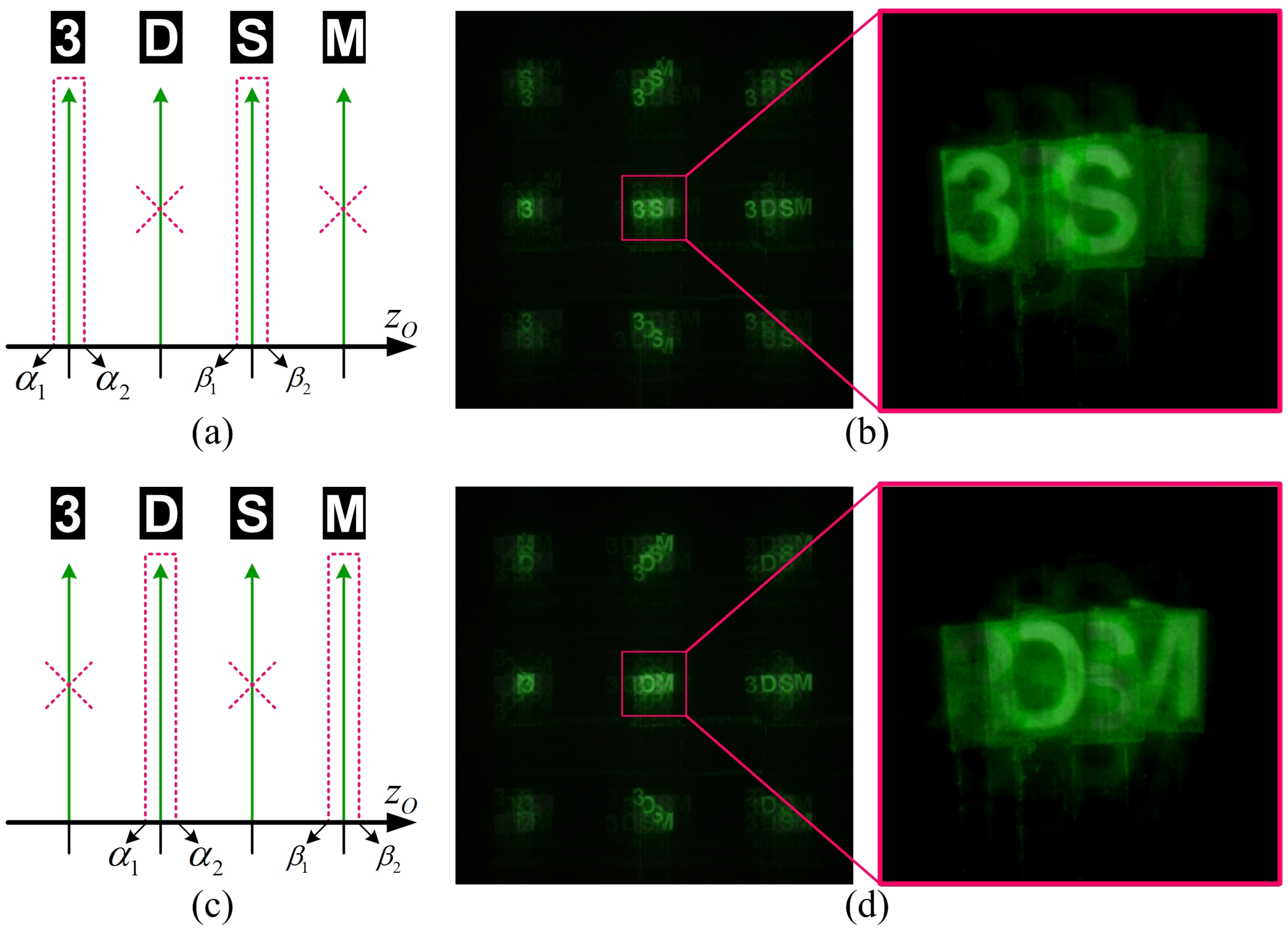
Next, we want to present the outcomes of our proposed spatial filtering method designed for multiple depths. Our spatial filtering results corresponding to the required depth range from the DIA are illustrated in Figure 5. Figure 5a,c depict the depth regions where spatial filtering for multiple depths will be conducted, as per Equation (9). Figure 5b is the result of the spatial filtering process, which is the calculation result of a definite integral over the range −99.5 mm $\le z_O\le$−100.5 mm for the Arabic numeral of ‘3’ and −109.5 mm $\le z_O\le$−110.5 mm for alphabet letter ‘S’ in Equation (9). Figure 5d is also the result of the spatial filtering process, which is the definite integral over the range −119.5 mm $\le z_O\le$−120.5 mm for the alphabet letter ‘D’ and −129.5 mm $\le z_O\le$−130.5 mm for the alphabet letter ‘M’ in Equation (9). To demonstrate the capability of selective depth extraction, we applied spatial filtering to extract depths corresponding to objects ‘3’ and ‘S’, even though the order of the objects is ‘3’, ‘D’, ‘S’, and ‘M’. Also, spatial filtering corresponding to the depth ranges of ‘D’ and ‘M’ was performed. Figure 5b,d are the results of spatial filtering for multiple depths based on Equation (9). These illustrate the results of convolving the DIA with an array of delta functions corresponding to multiple-depth ranges. On the left side of Figure 5b,d, the result of convolving the DIA with the delta function array is depicted, while the right side showcases an enlarged view of the 0th-order region (the center part) of our spatial filtering result. As evident from the spatially filtered DI in Figure 5, our method facilitates a three-dimensional reconstruction of the object space across multiple-depth regions, achieved by simultaneously and selectively controlling the depth range of spatial filtering.

Upon comparing Figure 4b with Figure 5b, it is apparent that the proposed CEMD method may introduce increased blur noise in the resultant images. This blurriness is influenced by both the proximity and number of neighboring objects. Specifically, when neighboring objects are closer to the target object’s depth and there are numerous neighboring objects, the blur noise tends to escalate. Consequently, Figure 5b exhibits more blur noise due to spatial filtering being conducted at two distinct target object depths. Moreover, the spatial filtering was conducted using a three-by-three array of the DIs in the DIA, resulting in a limited number of parallax images being utilized. Given the convolution operation detailed in Equations (8) and (9), as the number of DIs increases, the intensity of the 0th-order region is accentuated in the spatially filtered output. Hence, augmenting the number of DIs can mitigate the blurring effect in the reconstructed image. Objects with adjacent depths can increase noise in the reconstructed image even if they have separate depth resolutions because the difference in the spatial periods they occupy within the DIA is small. Therefore, it is necessary to establish the minimum depth between objects that corresponds to an acceptable noise level and its relationship with the number of DIs. The depth resolution of diffraction grating imaging is proportional to the spatial resolution of the image-acquisition device, such as imaging systems based on repoint imaging. The depth resolution of systems based on lens arrays, such as integral imaging, has a high depth resolution in close proximity to the lens array but decreases rapidly with distance. In contrast, the depth resolution of diffraction grating imaging is constant regardless of the depth of the object because it is linear, as implied by Equation (10). This characteristic of diffraction grating imaging has applications in depth-sensing cameras. In addition, the characteristic of having a high depth resolution can be applied to microscope imaging systems as far as the diffraction limit of the diffraction grating allows.

5. Conclusions

In conclusion, we introduced a novel approach in diffraction grating imaging to simultaneously reconstruct slice images corresponding to multiple-depth regions through a single controllable spatial filtering process. Through theoretical analysis, we derived mathematical grounds for applying the CEMD to diffraction grating imaging. For experimental verification, DIA was obtained optically, and spatial filtering for the 3D image was performed for the proposed method based on the theoretical analysis. The efficacy of the proposed method was validated through experimental reconstructions of partially occluded objects. The experiments demonstrate that our method offers selective control over the depth range for spatial filtering. We anticipate that the proposed method will be useful in diverse applications for diffraction grating imaging.

References

1. Lippmann, G. La photographie integrale. C. R. Acad. Sci. 1908, 146, 446–451. [Google Scholar]
2. Joshi, R.; Krishnan, G.; O’Connor, T.; Javidi, B. Signal detection in turbid water using temporally encoded polarimetric integral imaging. Opt. Exp. 2020, 28, 36033–36045. [Google Scholar] [CrossRef]
3. Jang, J.-S.; Javidi, B. Three-dimensional synthetic aperture integral imaging. Opt. Lett. 2002, 13, 1144–1146. [Google Scholar] [CrossRef]
4. Xiao, X.; Javidi, B.; Martinez-Corral, M.; Stern, A. Advances in three-dimensional integral imaging: Sensing, display, and applications [Invited]. Appl. Opt. 2013, 52, 546–560. [Google Scholar] [CrossRef]
5. Wani, P.; Usmani, K.; Krishnan, G.; Javidi, B. 3D object tracking using integral imaging with mutual information and Bayesian optimization. Opt. Exp. 2024, 32, 7495–7512. [Google Scholar] [CrossRef]
6. Wani, P.; Krishnan, G.; O’Connor, T.; Javidi, B. Information theoretic performance evaluation of 3D integral imaging. Opt. Exp. 2022, 30, 43157–43171. [Google Scholar] [CrossRef]
7. Sedick, R.; Guillaume, A.; Rosalie, T.; Simon, T. Orthoscopic elemental image synthesis for 3D light field display using lens design software and real-word captured neural radiance field. Opt. Exp. 2024, 32, 7800–7815. [Google Scholar]
8. Ma, H.; Yao, J.; Gao, Y.; Liu, J. Parameter optimization method for light field 3D display. Opt. Exp. 2023, 31, 42206–42217. [Google Scholar] [CrossRef] [PubMed]
9. Levoy, M. Light fields and computational imaging. IEEE Comput. Mag. 2006, 39, 46–55. [Google Scholar] [CrossRef]
10. Martinez-Corral, M.; Javidi, B. Fundamentals of 3D imaging and displays: A tutorial on integral imaging, light-field, and plenoptic systems. Adv. Opt. Photonics 2018, 3, 512–566. [Google Scholar] [CrossRef]
11. Hu, X.; Li, Z.; Miao, L.; Fang, F.; Jiang, Z.; Zhang, X. Measurement Technologies of Light Field Camera: An Overview. Sensors 2023, 23, 6812. [Google Scholar] [CrossRef]
12. Wu, G.; Masia, B.; Jarabo, A.; Zhang, Y.; Wang, L.; Dai, Q.; Chai, T.; Liu, Y. Light field image processing: An overview. IEEE J. Sel. Top. Signal Process. 2017, 11, 926–954. [Google Scholar] [CrossRef]
13. Jang, J.-Y.; Yoo, H. Computational Three-Dimensional Imaging System via Diffraction Grating Imaging with Multiple Wavelengths. Sensors 2021, 21, 6928. [Google Scholar] [CrossRef] [PubMed]
14. Jang, J.-Y.; Yoo, H. Image enhancement of Computational Reconstruction in Diffraction Grating Imaging Using Multiple Parallax Image Arrays. Sensors 2020, 20, 5137. [Google Scholar] [CrossRef] [PubMed]
15. Stantchev, R.I.; Mansfield, J.C.; Edginton, R.S.; Hobson, P.; Palombo, F.; Henry, E. Subwavelength hyperspectral THz studies of articular cartilage. Sci. Rep. 2018, 8, 6924. [Google Scholar] [CrossRef] [PubMed]
16. Cecconi, V.; Kumar, V.; Bertolotti, J.; Perters, L.; Cutrona, A.; Olivieri, L.; Pasquazi, A.; Totero Gongora, J.S.; Peccianti, M. Terahertz spatiotemporal wave synthesis in random systems. ACS Photonics 2024, 11, 362–368. [Google Scholar] [CrossRef] [PubMed]
17. Olivieri, L.; Peters, L.; Cecconi, V.; Cutrona, A.; Rowley, M.; Totero Gongora, J.S.; Pasquazi, A.; Peccianti, M. Terahertz nonlinear ghost imaging via plane decomposition: Toward near-field micro-volumetry. ACS Photonics 2023, 10, 1726–1734. [Google Scholar] [CrossRef] [PubMed]
18. Arai, J.; Okano, F.; Hoshino, H.; Yuyama, I. Gradient-index lens-array method based on real-time integral photography for three-dimensional images. Appl. Opt. 1998, 37, 2034–2045. [Google Scholar] [CrossRef]
19. Kim, H.; Hahn, J.; Lee, B. The use of a negative index planoconcave lens array for wide-viewing angle integral imaging. Opt. Exp. 2008, 16, 21865–21880. [Google Scholar] [CrossRef] [PubMed]
20. Jeong, Y.; Kim, J.; Yeom, J.; Lee, C.K.; Lee, B. Real-time depth controllable integral imaging pickup and reconstruction method with a light field camera. Appl. Opt. 2015, 54, 10333–10341. [Google Scholar] [CrossRef]
21. Wani, P.; Javidi, B. 3D integral imaging depth estimation of partially occluded objects using mutual information and Bayesian optimization. Opt. Exp. 2023, 31, 22863–22884. [Google Scholar] [CrossRef]
22. Li, H.; Wang, S.; Zhao, Y.; Wei, J.; Piao, M. 3D view image reconstruction in computational integral imaging using scale invariant feature transform and patch matching. Opt. Exp. 2019, 27, 24207–24222. [Google Scholar] [CrossRef] [PubMed]
23. Park, S.-G.; Yeom, J.; Jeong, Y.; Chen, N.; Hong, J.-Y.; Lee, B. Recent issues on integral imaging and its applications. J. Inf. Disp. 2013, 15, 37–46. [Google Scholar] [CrossRef]
24. Javidi, B.; Carnicer, A.; Arai, J.; Fujii, T.; Hua, H.; Liao, H.; Martínez-Corral, M.; Pla, F.; Stern, A.; Waller, L. Roadmap on 3D integral imaging: Sensing, processing, and display. Opt. Exp. 2020, 28, 32266–32293. [Google Scholar] [CrossRef] [PubMed]
25. Jang, J.-Y.; Cho, M.; Kim, E.-S. 3D image reconstruction with controllable spatial filtering based on correlation of multiple periodic functions in computational integral imaging. Chin. Opt. Lett. 2015, 13, 031101. [Google Scholar] [CrossRef]
26. Jang, J.Y.; Ser, J.I.; Kim, E.S. Wave-optical analysis of parallax-image generation based on multiple diffraction gratings. Opt. Lett. 2013, 38, 1835–1837. [Google Scholar] [CrossRef]
Figure 1. In the diffraction grating imaging system, the diffraction grating generates the ±1st-order DIs of the point object, which are then captured on the DIA pick-up plane by the imaging lens. (a) Geometric relation for a point object located at a single depth. (b) Geometric relation for two point objects located at different depths.
Electronics 13 01184 g001
Figure 2. (a) Experiment configuration and actual setup of diffraction grating imaging system. The object closest to the diffraction grating is located 100 mm away from the diffraction grating. The distance between the camera and the diffraction grating is 500 mm. (b) The objects used in the experiment are letters representing ‘3’, ‘D’, ‘S’, and ‘M’, and the distance between each object is 10 mm. (c) DIA acquired by a diffraction grating imaging system. Δ X is the spatial period, which increases with increasing depth of the object. (d) Enlarged part of 0th-order DI portion in the 3 × 3 PIA.
Electronics 13 01184 g002
Figure 3. (a) Position and spatial period of the objects in the diffraction grating system in the experiment. (b) Object depths of 100 mm to 110 mm vs corresponding spatial periods. The red rectangular area is a zoomed-in portion of the graph, where the spatial period is 10 pixels corresponding to a depth of 1 mm. The depth resolution is 0.1 mm of depth per 1 pixel of spatial period. (c) Spatial period corresponding to a depth of 120 mm to 130 mm.
Electronics 13 01184 g003
Figure 4. Spatial filtering used in the conventional method. (a) Filtering area, (b) spatially filtered DIA and its enlarged part.
Electronics 13 01184 g004
Figure 5. Spatial filtering used in the proposed method. (a) Filtering areas for letters ‘3’ and ‘S’, (b) spatially filtered DIA and its enlarged part, (c) filtering areas for letters ‘D’ and ‘M’, (d) spatially filtered DIA and its enlarged part.
Electronics 13 01184 g005
Disclaimer/Publisher’s Note: The statements, opinions and data contained in all publications are solely those of the individual author(s) and contributor(s) and not of MDPI and/or the editor(s). MDPI and/or the editor(s) disclaim responsibility for any injury to people or property resulting from any ideas, methods, instructions or products referred to in the content.