

Specific Emitter Identification through Multi-Domain Mixed Kernel Canonical Correlation Analysis
Abstract
:1. Introduction
2. Analysis of Canonical Correlation Analysis (CCA)
3. Kernel Methods
3.1. Kernel CCA
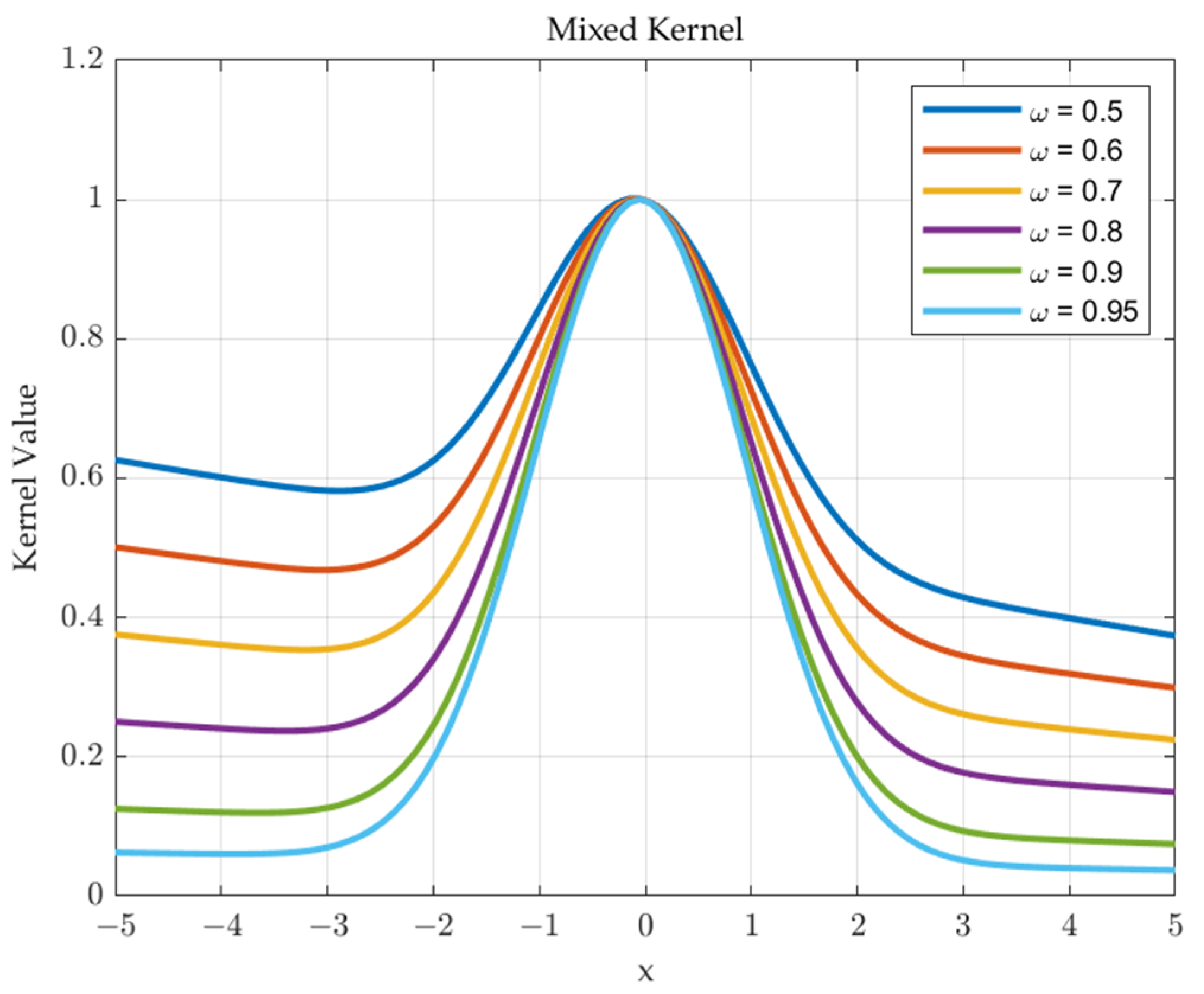
3.2. Mixed Kernel
3.3. Parameters Optimization
4. Experimental Analysis
4.1. Datasets
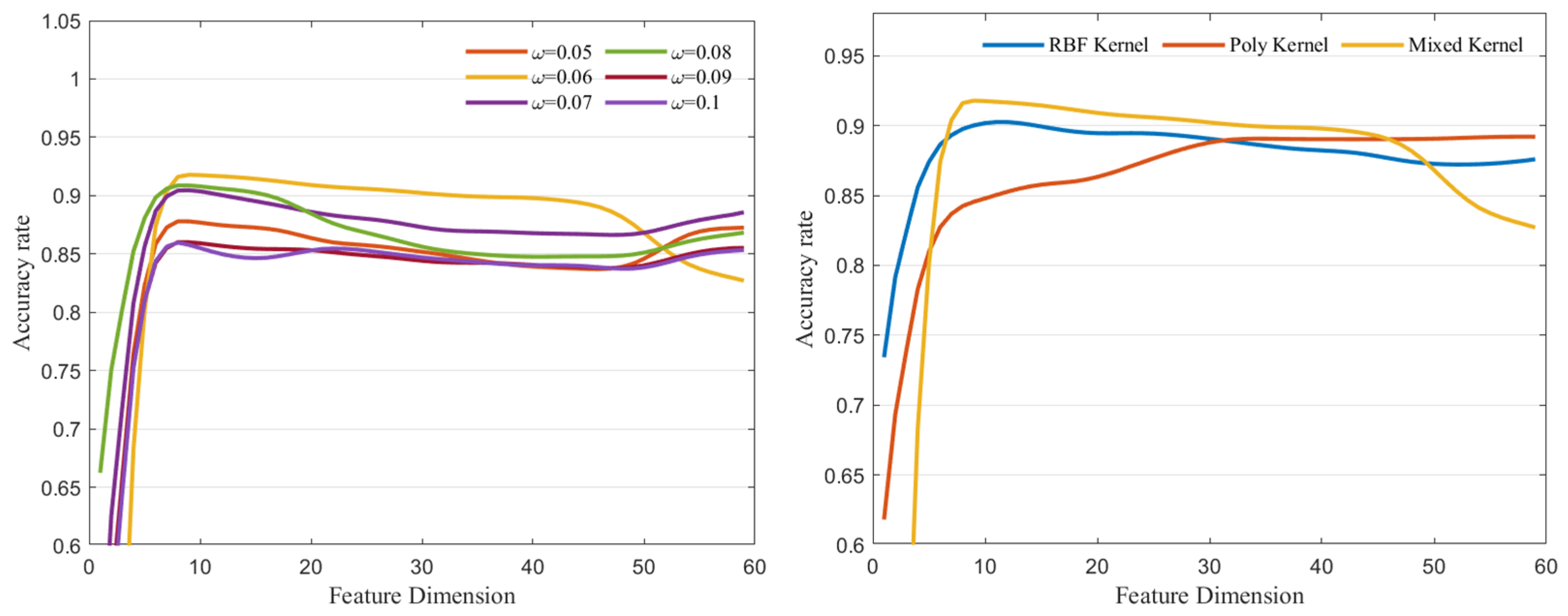
4.2. Kernel Function Analysis
4.3. Multi-Domain Feature Fusion Analysis
4.4. Performance Analysis
5. Summary
Author Contributions
Funding
Data Availability Statement
Conflicts of Interest
References
- Liu, Y.; Li, S.; Lin, X.; Gong, H.; Li, H. Feature Analysis and Extraction for Specific Emitter Identification Based on the Signal Generation Mechanisms of Radar Transmitters. Sensors 2022, 22, 2616. [Google Scholar] [CrossRef]
- Fu, X.; Peng, Y.; Liu, Y.; Lin, Y.; Gui, G.; Gacanin, H.; Adachi, F. Semi-Supervised Specific Emitter Identification Method Using Metric-Adversarial Training. IEEE Internet Things J. 2023, 10, 10778–10789. [Google Scholar] [CrossRef]
- Wang, Y.; Gui, G.; Gacanin, H.; Ohtsuki, T.; Dobre, O.A.; Poor, H.V. An Efficient Specific Emitter Identification Method Based on Complex-Valued Neural Networks and Network Compression. IEEE J. Sel. Areas Commun. 2021, 39, 2305–2317. [Google Scholar] [CrossRef]
- He, B.; Wang, F. Cooperative Specific Emitter Identification via Multiple Distorted Receivers. IEEE Trans. Inf. Forensics Secur. 2020, 15, 3791–3806. [Google Scholar] [CrossRef]
- Zhu, M.; Feng, Z.; Stanković, L.; Ding, L.; Fan, J.; Zhou, X. A probe-feature for specific emitter identification using axiom-based grad-CAM. Signal Process. 2022, 201, 108685. [Google Scholar] [CrossRef]
- Tan, K.; Yan, W.; Zhang, L.; Tang, M.; Zhang, Y. Specific Emitter Identification Based on Software-Defined Radio and Decision Fusion. IEEE Access 2021, 9, 86217–86229. [Google Scholar] [CrossRef]
- Zhao, Y.; Wang, X.; Lin, Z.; Huang, Z. Multi-Classifier Fusion for Open-Set Specific Emitter Identification. Remote Sens. 2022, 14, 2226. [Google Scholar] [CrossRef]
- Ali, A.M.; Uzundurukan, E.; Kara, A. Assessment of Features and Classifiers for Bluetooth RF Fingerprinting. IEEE Access 2019, 7, 50524–50535. [Google Scholar] [CrossRef]
- Suski Ii, W.C.; Temple, M.A.; Mendenhall, M.J.; Mills, R.F. Radio frequency fingerprinting commercial communication devices to enhance electronic security. Int. J. Electron. Secur. Digit. Forensics 2008, 1, 301–322. [Google Scholar]
- Ru, X.-H.; Liu, Z.; Huang, Z.-T.; Jiang, W.-L. Evaluation of unintentional modulation for pulse compression signals based on spectrum asymmetry. IET Radar Sonar Navig. 2017, 11, 656–663. [Google Scholar] [CrossRef]
- Li, L.; Ji, H.-B.; Jiang, L. Quadratic time–frequency analysis and sequential recognition for specific emitter identification. IET Signal Process. 2011, 5, 568–574. [Google Scholar] [CrossRef]
- Li, Y.-b.; Ge, J.; Lin, Y.; Ye, F. Radar emitter signal recognition based on multi-scale wavelet entropy and feature weighting. J. Cent. South Univ. 2014, 21, 4254–4260. [Google Scholar] [CrossRef]
- Mateo, C.; Talavera, J.A. Short-time Fourier transform with the window size fixed in the frequency domain. Digit. Signal Process. 2018, 77, 13–21. [Google Scholar] [CrossRef]
- Chen, J.; Xing, M.; Xia, X.G.; Zhang, J.; Liang, B.; Yang, D.G. SVD-Based Ambiguity Function Analysis for Nonlinear Trajectory SAR. IEEE Trans. Geosci. Remote Sens. 2021, 59, 3072–3087. [Google Scholar] [CrossRef]
- Liu, Z.-M. Multi-feature fusion for specific emitter identification via deep ensemble learning. Digit. Signal Process. 2021, 110, 102939. [Google Scholar] [CrossRef]
- Hou, K.; Li, N. Specific emitter identification based on CNN. J. Phys. Conf. Ser. 2021, 1971, 012014. [Google Scholar] [CrossRef]
- Zhang, X.; Li, T.; Gong, P.; Zha, X.; Liu, R. Variable-Modulation Specific Emitter Identification With Domain Adaptation. IEEE Trans. Inf. Forensics Secur. 2023, 18, 380–395. [Google Scholar] [CrossRef]
- Yang, J.; Yang, J.-Y.; Zhang, D.; Lu, J.-F. Feature fusion: Parallel strategy vs. serial strategy. Pattern Recognit. 2003, 36, 1369–1381. [Google Scholar] [CrossRef]
- Tong, L.; Fang, M.; Xu, Y.; Peng, Z.; Zhu, W.; Li, K. Specific Emitter Identification Based on Multichannel Depth Feature Fusion. Wirel. Commun. Mob. Comput. 2022, 2022, 9342085. [Google Scholar] [CrossRef]
- He, F.; Zhang, Z. Nonlinear Fault Detection of Batch Processes Using Functional Local Kernel Principal Component Analysis. IEEE Access 2020, 8, 117513–117527. [Google Scholar] [CrossRef]
- Jia, M.; Xu, H.; Liu, X.; Wang, N. The optimization of the kind and parameters of kernel function in KPCA for process monitoring. Comput. Chem. Eng. 2012, 46, 94–104. [Google Scholar] [CrossRef]
- Shiju, S.S.; Salim, A.; Sumitra, S. Multiple kernel learning using composite kernel functions. Eng. Appl. Artif. Intell. 2017, 64, 391–400. [Google Scholar]
- Pilario, K.E.S.; Cao, Y.; Shafiee, M. Mixed kernel canonical variate dissimilarity analysis for incipient fault monitoring in nonlinear dynamic processes. Comput. Chem. Eng. 2019, 123, 143–154. [Google Scholar] [CrossRef]
- Zhu, X.; Huang, Z.; Tao Shen, H.; Cheng, J.; Xu, C. Dimensionality reduction by Mixed Kernel Canonical Correlation Analysis. Pattern Recognit. 2012, 45, 3003–3016. [Google Scholar] [CrossRef]
- Gao, X.; Niu, S.; Sun, Q. Two-Directional Two-Dimensional Kernel Canonical Correlation Analysis. IEEE Signal Process. Lett. 2019, 26, 1578–1582. [Google Scholar] [CrossRef]
- Yoshida, K.; Yoshimoto, J.; Doya, K. Sparse kernel canonical correlation analysis for discovery of nonlinear interactions in high-dimensional data. BMC Bioinform. 2017, 18, 108. [Google Scholar] [CrossRef]
- Hardoon, D.R.; Szedmak, S.; Shawe-Taylor, J. Canonical Correlation Analysis: An Overview with Application to Learning Methods. Neural Comput. 2004, 16, 2639–2664. [Google Scholar] [CrossRef]
- Guo, S.; Sheng, Y.; Chai, L.; Zhang, J. PET Image Reconstruction with Kernel and Kernel Space Composite Regularizer. IEEE Trans. Med. Imaging 2023, 42, 1786–1798. [Google Scholar] [CrossRef]
- Cai, J.; Tang, Y.; Wang, J. Kernel canonical correlation analysis via gradient descent. Neurocomputing 2016, 182, 322–331. [Google Scholar] [CrossRef]
- Pu, Y. Morphological Feature Extraction Based on the Polar Transformation of the Slice of Ambiguity Function Main Ridge. Yi Qi Yi Biao Xue Bao/Chin. J. Sci. Instrum. 2018, 39, 1–9. [Google Scholar]
- Wan, T.; Ji, H.; Xiong, W.; Tang, B.; Fang, X.; Zhang, L. Deep Learning-Based Specific Emitter Identification Using Integral Bispectrum and the Slice of Ambiguity Function. Signal Image Video Process. 2022, 16, 2009–2017. [Google Scholar] [CrossRef]


| : metric spaces | : inner product |
| : feature vector | : Lagrange function |
| : the linear transformation of x | : kernel matrix |
| : the linear transformation of y | : a map into Hilbert spaces |
| : correlation coefficient | : correlations |
| : covariance metric | : fusion feature vector |
| Kernel Function | Mixed Kernel | RBF Kernel | Poly Kernel |
|---|---|---|---|
| Time (s) | 4.1131 | 4.9133 | 3.8902 |
| Method | CCA | Poly CCA | RBF CCA | KPCA | MKCCA |
|---|---|---|---|---|---|
| Time(s) | 28.543 | 15.116 | 22.797 | 40.237 | 19.729 |
Disclaimer/Publisher’s Note: The statements, opinions and data contained in all publications are solely those of the individual author(s) and contributor(s) and not of MDPI and/or the editor(s). MDPI and/or the editor(s) disclaim responsibility for any injury to people or property resulting from any ideas, methods, instructions or products referred to in the content. |
© 2024 by the authors. Licensee MDPI, Basel, Switzerland. This article is an open access article distributed under the terms and conditions of the Creative Commons Attribution (CC BY) license (https://creativecommons.org/licenses/by/4.0/).
Share and Cite
Chen, J.; Li, S.; Qi, J.; Li, H. Specific Emitter Identification through Multi-Domain Mixed Kernel Canonical Correlation Analysis. Electronics 2024, 13, 1173. https://doi.org/10.3390/electronics13071173
Chen J, Li S, Qi J, Li H. Specific Emitter Identification through Multi-Domain Mixed Kernel Canonical Correlation Analysis. Electronics. 2024; 13(7):1173. https://doi.org/10.3390/electronics13071173
Chicago/Turabian StyleChen, Jian, Shengyong Li, Jianchi Qi, and Hongke Li. 2024. "Specific Emitter Identification through Multi-Domain Mixed Kernel Canonical Correlation Analysis" Electronics 13, no. 7: 1173. https://doi.org/10.3390/electronics13071173