Diagnosis of Analog Circuits: The Problem of Ambiguity of Test Equation Solutions

Abstract

Diagnosis of analog electronic circuits is a crucial issue in computer-aided design. During the diagnosis, solving a test equation to identify the values of faulty parameters is usually necessary. The equation is nonlinear to the parameters, even for linear circuits. The nonlinearity of the equation implies the possibility of multiple solutions. No method exists that guarantees the determination of all the solutions of the test equation. However, even information about more than one existing solution is essential for the designer. It allows for the selection of another test at the design step and helps to obtain an unambiguous solution during the diagnosis. Information about the possibility of additional solutions is essential for simulation after test methods (e.g., identification and verification methods) and for simulation before test methods, so-called dictionary methods, especially those targeting multiple fault classification. The paper deals with the problem of multiple solutions of the test equation for nonlinear DC circuits and proposes a method for identifying the solutions using a deflation technique. The outcomes are compared with the results obtained using standard and adaptively damped Newton–Raphson iterative methods. The methods use randomly selected initial guesses to find multiple solutions. The effectiveness of all the methods for identifying multiple solutions was verified numerically and via laboratory tests.

1. Introduction

The development of integrated circuit and semiconductor technology in the second half of the last century has led to a growing interest in computer-aided design of nonlinear circuits and systems. The most critical problems that research and development centers have tried to solve are the elaboration of efficient algorithms to analyze the circuits and methods to design for testing (DfT). Even the early simulators, such as CANCER, SPICE1, and NAP, made it possible to determine solutions for nonlinear circuits using simple semiconductor models, e.g., Ebers–Moll for a bipolar transistor. Technological developments, especially in CMOS technology, have led to the use of complex, multi-parameter transistor models, e.g., the PSP or BSIM one. In the meantime, many papers have highlighted potential problems in the simulation and operation of nonlinear circuits. Researchers have focused particular attention on the issue of multiple solutions and chaos [1,2,3,4,5,6,7,8,9]. Simultaneously, research was performed on the automation of testing different classes of circuits [10,11,12,13,14,15,16,17,18,19,20,21,22,23,24,25,26,27,28,29,30,31,32,33,34,35,36,37,38,39,40,41,42,43,44,45,46,47,48,49]. Standards have been developed for digital circuits, significantly improving the diagnostic process. Unfortunately, the same issue for analog circuits has lagged. The reason is the continuity of analog signals, noise from various external sources, and parameter tolerances, which affect the diagnostic results. Moreover, various faults of individual components exist, i.e., parametric/soft faults (parameter value out of tolerance range) and catastrophic/hard faults (leading to topology changes resulting from short or open circuits). Limited access to the interior terminals of the circuit to excitation or measurement facilities further complicates the performance of a successful diagnosis. Thus, the step of proper test selection, maximizing the effectiveness of the diagnostic methods, is crucial [27]. Since universal diagnostic methods have not been developed, a split in methods into two classes is made: so-called methods with before-test simulation (SBT) and methods with after-test simulation (SAT). The SBT methods mainly focus on fault detection (go/no-go test) and on classification of single faults (indicating which component is faulty). Some SBT methods allow a faulty parameter up or down deviation from a nominal value classification or even localization of selected multiple faults. Artificial intelligence methods, including various neural networks, are typically used as fault classifiers in SBT methods [18,28,30,31,32,39,47,48,49]. These methods indicate faults of each class with high precision, up to 100%. Unfortunately, the nature of the SBT methods makes the approaches only of limited use at the design stage, where it is necessary to identify multiple soft faults. In such cases, the typical approach is to use SAT methods. The group of methods includes identification, verification, and optimization methods [17,27,32,40,41,42]. SAT methods typically lead to a nonlinear test equation whose solution (or solutions) meets measurement readings. SAT methods allow for determining the values of more parameters than the SBT approaches, but require more diagnostic information.

Although the analysis and SAT diagnosis of circuits involve different aspects and applications, these topics for nonlinear circuits have a common aspect. The aspect is the need to solve systems of nonlinear equations. In DC analysis, a specific description of the circuit, e.g., a modified nodal or hybrid description, leads to the equation. The solution for the system at constant values of the element parameters is found using a numerical method, e.g., the Newton–Raphson method or the Piccard method. As a result, the values of nodal voltages, branch voltages, and currents are obtained. In the fault diagnostic method, the problem is posed differently. Based on the measured values of the circuit quantities (voltages/currents), a nonlinear equation called the test equation is formed and solved. The solutions to the equation are the values of element parameters. The number of parameters sought is usually greater than the number of measured quantities at a single excitation. Thus, it is necessary to consider the results of measurements at several different excitations. The test equation is generally nonlinear, even for linear circuits.

Both finding all solutions in nonlinear circuits and determining parameter values in fault diagnosis require solving a system of nonlinear equations, briefly referred to as a nonlinear equation. Thus, it is crucial to consider the possibility of multiple solutions to this equation when developing reliable analysis and testing methods. In analysis, multiple solutions mean that the same circuit has different voltage/current values (so-called equilibrium points) depending on the initial conditions of the associated dynamic circuit. In diagnosis, multiple solutions mean that different sets of parameters or even, as shown in the article [41], and that the same parameters but with different values satisfy the test. Eliminating the undesirable and potentially misleading solutions requires choosing a new test. Therefore, an important issue is identifying multiple solutions already at the design step. At this stage, it is possible to provide sufficient access for measurements. The problem is essential in SAT and SBT methods, where fault classification is based on a given test. The most complicated diagnostic case concerns the testing of circuits with multiple DC solutions [43].

The paper proposes a quick and easy-to-implement procedure to identify multiple solutions to test equations. Identification is understood as the statement of whether multiple solutions to a diagnostic equation are possible based on measurement data (for a measurement test established at the design stage). The appearance of multiple solutions at the DfT stage makes it possible to rearrange the test to obtain an unambiguous diagnosis at the actual circuit testing step. Therefore, the input data are the results of CUT simulations at a predefined test for different parametric faults, and the result of the computational procedure is to conclude whether the obtained solution of the test equation is unambiguous. In addition, the software results in parameter values corresponding to the various solutions. The procedure can be helpful at the step of selecting a test for both SAT and SBT methods. Section 2 reviews existing methods dealing with the problem of multiple solutions in circuit analysis and diagnosis. Section 3 discusses the numerical techniques and methods used in the paper, particularly the concept of deflation. Section 4 illustrates the effectiveness of the methods to identify multiple solutions of the test equation in nonlinear circuits, through numerical simulations and laboratory tests. Section 5 concludes the obtained results.

2. Multiple Solutions in the Analysis and Diagnosis of Electronic Circuits

Robust and efficient determination of solutions to systems of nonlinear equations is a challenging problem from a theoretical and practical point of view. Calculating DC solutions is one of the most critical tasks when analyzing electronic circuits [1,2,3,4,5,6,7,8,9]. The Newton–Raphson method and its variants are used in standard simulators to compute solutions to the equations describing the analyzed circuits. The methods can reach quadratic or super-linear convergence by taking the initial guess near the solution. Once one solution is found, the computational process is terminated, and the user is not given any information about the possibility that other solutions exist. Therefore, the methods are not suited for calculating multiple solutions. However, a lot of circuits have many isolated operating points [7,8]. It is crucial to verify the points before the circuit is manufactured. Determining the points is also essential when studying chaos [2].

Finding multiple solutions in nonlinear DC circuits is a difficult task. Two approaches to the problem exist in the literature. The first approach relies on methods that guarantee finding all solutions [3,5,6]. The methods usually require a specific hybrid description, can be applied to circuits belonging to a strictly defined class, and use simple models of semiconductor devices. The most commonly used approaches are based on computational techniques using piecewise-linear approximation (PWL) [5]. However, the methods have limited accuracy due to the approximation. For reliable results, it is necessary to analyze the original nonlinear circuits. Interval methods and approaches based on the idea of successive contraction, division, and elimination of certain hyper-rectangular regions where solutions are sought can be applied here [1,3,6]. The complexity of the numerical procedures and the time-consuming aspect make the problem of finding all solutions for a large-scale circuit still unsolved. The issue remains pending and will be a challenge in the future, according to many researchers. Therefore, other approaches focus on identifying only some solutions, although sometimes they allow finding all solutions. For this purpose, the concept of homotopy [7,8], the idea of deflation [2], evolutionary computation, and the Carleman linearization [9] are proposed. A separate class of methods consists of algorithms that identify the possibility of multiple solutions in nonlinear circuits by searching for specific topological structures [4].

SAT methods are usually aimed at soft fault diagnosis. They usually allow for the location of faulty components and the evaluation of their actual parameters. For this purpose, a system of nonlinear diagnostic equations of algebraic type is formulated and solved. When the parameters are slightly outside the tolerance region, the equation can be linearized, leading to an unambiguous solution, provided testability is considered (the testability concept will be explained later in this section). However, such procedures lead to approximate parameter values. More accurate results are obtained using methods for solving the original nonlinear equations, such as the Newton–Raphson method or its variants. Finding solutions to the test equation becomes more challenging when parameter changes are significant. In such a case, some methods fail to converge, or they converge to unphysical solutions. Furthermore, several sets of parameters may then satisfy the test equation. In the area of diagnostics, in contrast to DC analysis, to the author’s knowledge, no method guarantees the determination of all solutions. In order to find some of the solutions, various initial guesses may be chosen, and standard methods used. Such an approach was first proposed in [20]. Another method based on the homotopy concept and an efficient procedure for tracing a homotopy path was proposed in [40]. In a systematic manner, it can find several sets of parameters that satisfy the diagnostic test rather than one specific set. However, the computational process is complex and challenging to implement, and numerical examples show that the method diverges in about 10% of cases. A systematic search method was developed in [41] to find multiple solutions to the test equation in BJT and MOS circuits. The algebraic test equation is transformed into an initial value problem (IVP). The IVP is solved by numerical integration, so the computational process is complex, although, as the results in [41] show, it is efficient. All the methods discussed above are so-called verification methods, and deal with DC nonlinear circuits. The methods are based on the assumption that the faulty elements are known and usually limited to a few parameters. The remaining elements are assumed to be healthy. Using a redundant number of measurements relative to the number of parameters sought, so as to avoid multiple solutions, was also applied in [42] to diagnose soft faults in linear AC systems. The proposed algorithm solves the problem using the Levenberg–Marquardt method. Unlike verification methods, the algorithm is applied to all testable element sets.

The testability of a circuit is an important issue in the study of solution ambiguity [10,11,14,15,16,19,21,22,23,24,25,29,37,38,44,45]. Testability has been the subject of intensive research since the 1960s, and methods in this area deal mainly with linear circuits. Testability provides theoretical and rigorous upper bounds on the degree of solvability of a problem once a set of test points has been selected. Various approaches based on fully numerical, symbolic, or graphical techniques are available for linear (or linearized at the operating point) circuits [14]. An important concept is the ambiguity group. If considered potentially faulty, this set of components does not provide a unique solution when identifying a fault at the chosen test. An ambiguity group that does not contain other ambiguity groups is called a canonical ambiguity group. Typical testability identification procedures are well established and use the Jacobian matrix rank evaluation of the test equation. Testability analysis in nonlinear circuits is much more complex. The article [19] proposes a procedure for determining testability and ambiguity groups for analog circuits containing nonlinear devices. The proposed approach uses the idea of piecewise linear approximation of nonlinear characteristics and considers combinations of linearity regions using testability evaluation techniques for linear circuits. However, the method has practical application only for relatively simple circuits. Testability in fault diagnosis of DC–DC converters considering the single fault hypothesis is discussed in [10,14]. The approach proposed in [10] is based on symbolic analysis techniques for linear circuits corresponding to a specific operating phase (i.e., a specific switch state). In [14], a graphical testability evaluation is additionally used. Thus, the problem of testability for nonlinear circuits is still open.

Thus, as can be seen from the literature review presented, the problem of multiple solutions in nonlinear circuits has been addressed in several works. However, most of the works are of a verification type. They do not give a complete insight into the phenomenon’s scale when comprehensively looking at the circuit under test. Furthermore, the computational effort required to verify a single set of several parameters is considerable. Therefore, the paper attempts to develop a simple and efficient procedure to identify multiple solutions in the diagnosis of nonlinear circuits.

3. Solving the Nonlinear Test Equation

3.1. Preliminaries

In this paper, only single and multiple soft faults are considered. Hard faults can be effectively localized using dictionary methods and properly learned classifiers due to their usually significant impact on the measured quantities. A general form of the nonlinear test equation for soft faults is defined first. For circuits consisting of n parameters considered potentially faulty, the diagnostic test is arranged according to the test domain. For nonlinear DC circuits, the circuit under test (CUT) is driven by a voltage (current) source or sources applied to the terminals available for excitation, and the output voltages (currents) are read at the nodes (branches) available for measurement. If the number of measurements is less than n, the measurement is repeated for a different source(s) value to obtain at least n values of the circuit quantities. For linear (or linearized at operating point nonlinear circuits) considered in the AC domain, CUT is usually driven by a source applied to the input terminals. Measurements of the rms value and phase of the output voltage are taken at the nodes available for measurement at fixed test frequencies to obtain at least n measurement values. For circuits considered in the time domain, CUT is driven by a waveform produced by a signal generator, e.g., a DDS generator. Measured output voltage (current) values are read at the nodes (branches) available for measurement at fixed instants of time to obtain at least n of measured values.

The measured voltage (current) values form a vector $\mathbf{q}={\left[q_1\cdots q_n\right]}^{\mathrm{T}}$, where $\mathrm{T}$ denotes the transposition. Each measured circuit quantity is a certain function of the parameters $x_1,\cdots ,x_n$, $q_i={\widehat{f}}_i\left(\mathbf{x}\right)$, $i=1,\cdots ,n$, where $\mathbf{x}={\left[x_1{x}_2\cdots x_n\right]}^{\mathrm{T}}$. The parameters forming vector $\mathbf{x}$ depend on the class of circuits and the test domain. In the case of DC nonlinear circuit diagnosis, the parameters can include resistance and model parameters of nonlinear semiconductor devices such as saturation current, dependent source gain coefficient, and transconductance. The above scalar relations can be written in vector form as $\widehat{\mathbf{f}}\left(\mathbf{x}\right)=\mathbf{q}$, where $\widehat{\mathbf{f}}\left(\mathbf{x}\right)={\left[{\widehat{f}}_1\left(\mathbf{x}\right)\cdots {\widehat{f}}_n\left(\mathbf{x}\right)\right]}^{\mathrm{T}}$. The equation is usually written in the form

$$\mathbf{f}\left(\mathbf{x}\right)=\mathbf{0},$$

(1)

where $\mathbf{f}\left(\mathbf{x}\right)=\widehat{\mathbf{f}}\left(\mathbf{x}\right)-\mathbf{q}$, $\mathbf{0}={\left[00\cdots 0\right]}^{\mathrm{T}}$. Equation (1) is called the test equation. In real circuits, the nonlinear function $\widehat{\mathbf{f}}\left(\mathbf{x}\right)$ is not known in explicit analytical form.

From a mathematical point of view, the test Equation (1) may have multiple solutions. Unfortunately, no method guarantees the finding of all the solutions. Therefore, the following sections discuss several methods that may lead to some of the solutions. The methods described in the first two subsections are iterative and find one solution based on a single initial guess. The first method is the standard Newton–Raphson method, commonly used in solving systems of nonlinear equations. Properly selecting the initial guess leads to a quadratic convergence to the solution. However, an incorrectly chosen initial guess can result in slow convergence or divergence. The second method is a modified Newton–Raphson method, which is more robust to the problem of divergence and poorly chosen initial guesses [50], (p. 192). However, in cases where the standard Newton–Raphson method iterates from a good initial guess, the modified method usually requires more iterations. Both methods are run many times from randomly selected initial guesses (1000 guesses assumed) to find multiple solutions. Each new solution is stored. The results of these calculations were compared with the results of the method based on the deflation technique proposed in Section 3.6. The idea of deflation is discussed in Section 3.4. An example illustrating how the methods work is discussed in Section 3.5.

3.2. The Standard Newton–Raphson Method (S-NRM)

In this section, the standard Newton–Raphson method (S-NRM) applied to a system of n equations written in the form (1) having a solution ${\mathbf{x}}^{*}={\left[x_1^{*}{x}_2^{*}\cdots x_n^{*}\right]}^{\mathrm{T}}$ is discussed. Assuming that the functions $f_i\left(\mathbf{x}\right)$, $i=1,\cdots ,n$, are sufficiently smooth and expanding them into a Taylor series around some point ${\mathbf{x}}^{\left(j\right)}={\left[x_1^{\left(j\right)}{x}_2^{\left(j\right)}\cdots x_n^{\left(j\right)}\right]}^{\mathrm{T}}$ after elementary rearrangements, the following relation defining the Newton–Raphson iterative process is derived

$$\mathbf{J}\left({\mathbf{x}}^{\left(j\right)}\right)\left({\mathbf{x}}^{\left(j+1\right)}-{\mathbf{x}}^{\left(j\right)}\right)=-\mathbf{f}\left({\mathbf{x}}^{\left(j\right)}\right),$$

(2)

where $\mathbf{J}\left({\mathbf{x}}^{\left(j\right)}\right)$ is the Jacobi matrix. The iterative process involves solving Equation (2) for ${\mathbf{x}}^{\left(j+1\right)}$ using the previously calculated ${\mathbf{x}}^{\left(j\right)}$. The iterative process starts from an assumed initial guess ${\mathbf{x}}^{\left(0\right)}$. By introducing an auxiliary designation ${\mathbf{y}}^{\left(j+1\right)}=\left({\mathbf{x}}^{\left(j+1\right)}-{\mathbf{x}}^{\left(j\right)}\right)$, a typical calculation process involves solving a linear equation

$$\mathbf{J}\left({\mathbf{x}}^{\left(j\right)}\right){\mathbf{y}}^{\left(j+1\right)}=-\mathbf{f}\left({\mathbf{x}}^{\left(j\right)}\right)$$

(3)

for ${\mathbf{y}}^{\left(j+1\right)}$ and determining the successive approximation of the solution from the formula

$${\mathbf{x}}^{\left(j+1\right)}={\mathbf{x}}^{\left(j\right)}+{\mathbf{y}}^{\left(j+1\right)}.$$

(4)

The procedure is repeated for $j=1,2,\dots ,$ until both conditions ${∥{\mathbf{y}}^{\left(j+1\right)}∥}_{\infty }<\epsilon$ and ${∥\mathbf{f}\left({\mathbf{x}}^{\left(j+1\right)}\right)∥}_{\infty }<\eta$ are met, where $\epsilon$ specifies an assumed error tolerance, $\eta$ is a sufficiently small number, e.g., $\epsilon ={10}^{-4}÷{10}^{-3}$, $\eta =0.001$, and ${∥·∥}_{\infty }$ is the uniform (infinity) norm. Choosing an initial guess that guarantees rapid convergence is generally a difficult task. If the sequence of successive iterations does not converge, the process is terminated, another initial guess is set, and the calculation is repeated.

3.3. The Damped Newton–Raphson Method (D-NRM)

In order to improve the convergence of S-NRM, a modification involving step reduction is often used. The simplest case is the damped version of the algorithm, which involves reducing the step in a certain ratio, leading to the following modification of (4),

$${\mathbf{x}}^{\left(j+1\right)}={\mathbf{x}}^{\left(j\right)}+\lambda {\mathbf{y}}^{\left(j+1\right)},$$

(5)

where $\lambda$ is the damping coefficient from the interval $\left(0,1\right]$. The main difficulty is the selection of a damping coefficient $\lambda$. In the simplest case, the coefficient is chosen arbitrarily and fixed. In more sophisticated software, the coefficient is changed at each iteration. If the initial guess is far from the solution, then the direction of convergence determined by the Jacobi matrix may be ill-defined. Such a phenomenon is characterized by successive solutions diverging in a zig-zag manner. It manifests in changing the sign of the elements of the vector ${\mathbf{y}}^{\left(j+1\right)}$. To prevent the phenomenon, ${\mathbf{x}}^{\left(j+1\right)}$ is calculated using the formula

$${\mathbf{x}}^{\left(j+1\right)}={\mathbf{x}}^{\left(j\right)}+{\lambda }^{\left(j\right)}{\mathbf{y}}^{\left(j+1\right)},$$

(6)

where ${\lambda }^{\left(j\right)}$ it is chosen as follows. If there is a change in sign, then ${\lambda }^{\left(j\right)}={\lambda }^{\left(j-1\right)}·\Theta$; otherwise, ${\lambda }^{\left(j\right)}={\lambda }^{\left(j-1\right)}/\phantom{{\lambda }^{\left(j-1\right)}\Theta }\Theta$, $\Theta$ is some constant chosen experimentally, ($\Theta <1$, e.g., 0.75). If ${\lambda }^{\left(j\right)}>1$, then ${\lambda }^{\left(j\right)}=1$ is taken. If ${\lambda }^{\left(j\right)}<0.001$, then ${\lambda }^{\left(j\right)}=0.001$ is taken. The above-described modification of the Newton–Raphson method will is called the damped Newton–Raphson method (D-NRM).

3.4. Deflation Technique (DT)

The proposed approach uses a concept known in mathematics as the deflation technique (DT) [2,51,52,53,54,55]. The theoretical foundations of DT are given in [51]. Farrell et al. extended the concept to systems of partial differential equations [52]. DT in application to finding the solution of a system of nonlinear equations at roots where the Jacobian is singular is discussed in [53]. Huang et al. proposed using DT to find eigenvalues in dispersive metallic photonic crystals [54]. Luo and Xiao presented an optimization method composed of DT, the continuation method, and quasi-genetic evolution [55]. Article [2] proposes a method for finding multiple operating points using the deflation technique and the SPICE simulator.

An interesting problem in solving nonlinear equations is the presence of [51]. The zero is the root to which the numerical process converges, regardless of the initial guess chosen. The problem often leads to the masking of the zero, which is essential for the actual study. DT makes it possible to avoid convergence to the magnetic zero once it has been found. It allows other solutions to the nonlinear equation to be found. The problem is illustrated using an elementary example in Section 3.5.

The idea of DT [51] is to modify the original equation continuously after determining its successive solution. The newly formulated nonlinear equation retains the solutions of the original equation that remain to be calculated, making it impossible for the numerical process to converge to the previously found solutions.

The nonlinear Equation (1) is considered under the assumption that the equation has several solutions. Let one of the solutions, denoted ${\mathbf{x}}^1$, has already been found. To determine the other solutions, Equation (1) is deformed. Paper [51] introduced a deflation matrix $\mathbf{M}\left(\mathbf{x},{\mathbf{x}}^1\right)$ of dimension n by n and proposed the deformation of the original function in the form

$$\mathbf{g}\left(\mathbf{x}\right)=\mathbf{M}\left(\mathbf{x},{\mathbf{x}}^1\right)\mathbf{f}\left(\mathbf{x}\right),$$

(7)

where, for any sequence ${\mathbf{x}}^{\left(i\right)}\to {\mathbf{x}}^1$, it holds ${lim}_{i\to \infty }inf\left|\right|\mathbf{M}\left({\mathbf{x}}^{\left(i\right)},{\mathbf{x}}^1\right)\mathbf{f}\left({\mathbf{x}}^{\left(i\right)}\right)\left|\right|>0$.

Equation (7) is solved using a method for determining a single solution (e.g., S-NRM or D-NRM). The selection of the matrix $\mathbf{M}$ guarantees that ${\mathbf{x}}^1$ is not a solution to (7). Thus, the sequence generated by the method is either convergent to another solution of the original Equation (1) or divergent. In order to deflate k solutions of ${\mathbf{x}}^1$, ⋯, ${\mathbf{x}}^k$, deflation is formulated in the form

$$\mathbf{g}\left(\mathbf{x}\right)=\mathbf{M}\left(\mathbf{x},{\mathbf{x}}^1\right)\cdots \mathbf{M}\left(\mathbf{x},{\mathbf{x}}^k\right)\mathbf{f}\left(\mathbf{x}\right).$$

(8)

The various deflation methods differ in the selection of $\mathbf{M}$. In the so-called normal deflation, $\mathbf{M}$ has the form

$$\mathbf{M}\left(\mathbf{x},{\mathbf{x}}^j\right)=\frac{1}{\left|\right|\mathbf{x}-{\mathbf{x}}^j\left|\right|}\mathbf{A},$$

(9)

where $\mathbf{A}$ is a $n\times n$ matrix, and $\left|\right|·\left|\right|$ denotes a norm, e.g., uniform or Euclidean norm. Usually, the identity matrix is chosen as the matrix $\mathbf{A}$.

Brown and Gearhart proposed the following strategy for determining multiple solutions [51]. The nonlinear equation is solved using the S-NRM or Brown method to locate the first solution. Next, DT is used to create the modified function. The deflations with uniform and Euclidean norm and the so-called gradient deflation are considered. The second solution is sought using the same initial guess. If the second solution is found, the process continues, always using the same initial guess. The process ends when (a) all solutions to the nonlinear equation (or the maximum number of solutions set by the user) have been found, (b) the process has become divergent, (c) the maximum allowed number of iterations has been exceeded, or (d) the Jacobi matrix became singular. A simple example in [51] shows that all solutions were determined for only one of 21 different initial guesses and one $\mathbf{M}$ in DT. Other examples in paper [51] show that the S-NRM often leads to divergence, even in the first solution calculation.

To the author’s knowledge, the deflation technique has not yet been applied in fault diagnosis, and the proposal presented in Section 3.6 is the first in this area.

3.5. Illustrative Example

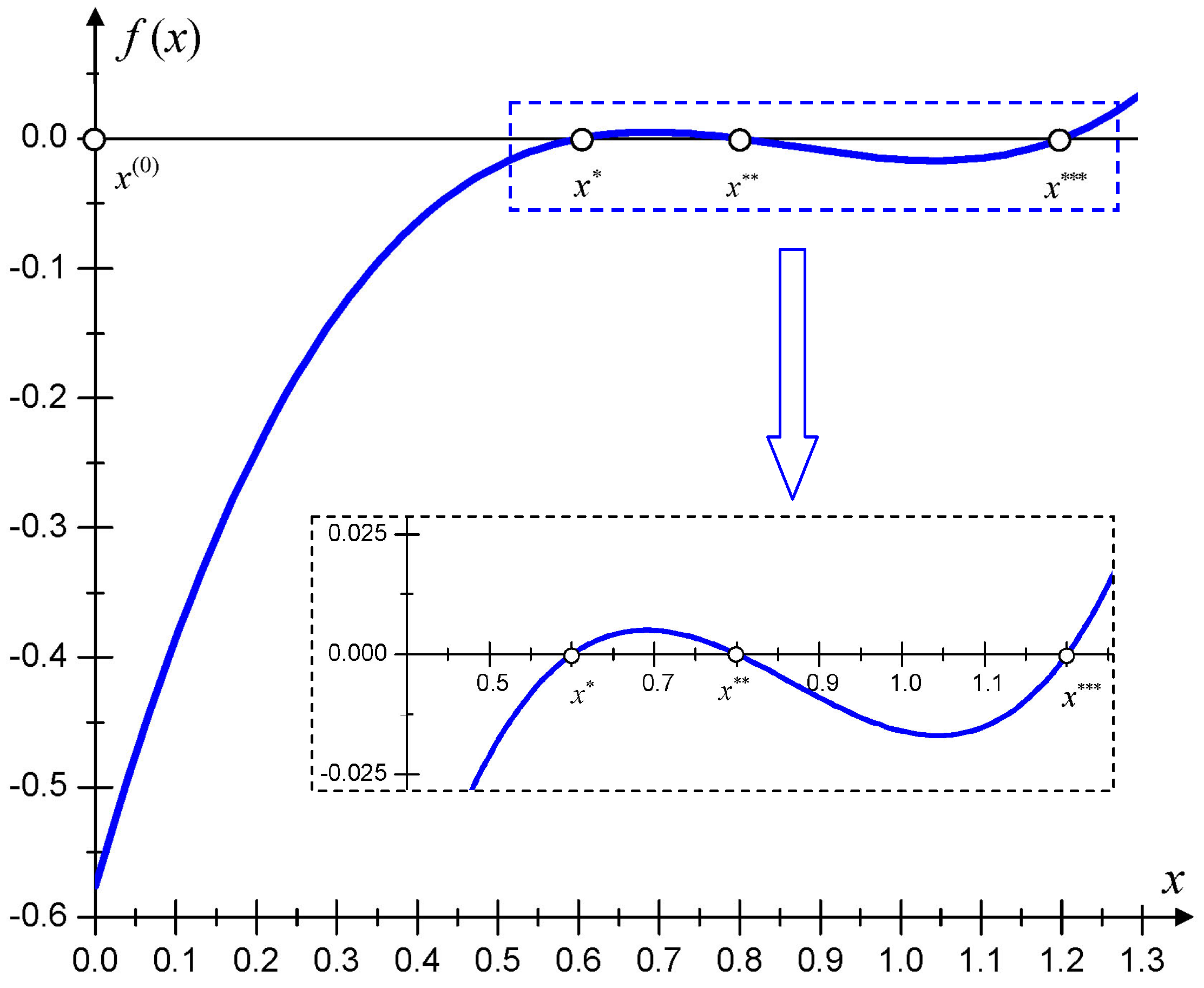
To illustrate the application of the methods discussed in Section 3.2, Section 3.3 and Section 3.4, the solutions of a scalar nonlinear equation $f\left(x\right)=0$ with $f\left(x\right)$ having the form

$$f\left(x\right)=x^3-2.6x^2+2.16x-0.576$$

(10)

are considered. Equation (10) is written in the equivalent form

$$f\left(x\right)=\left(x-0.8\right)\left(x-0.6\right)\left(x-1.2\right),$$

(11)

from which it follows that its roots are $x^{*}=0.6$, $x^{**}=0.8$, and $x^{***}=1.2$ (see Figure 1). Three methods were used: S-NRM, D-NRM, and DT. For S-NRM and D-NRM, 1000 draws of the initial guess $x^{\left(0\right)}$ were made using the uniform distribution. In case (a), initial guesses are drawn from the interval $(-0.5,0.5)$, and in case (b), from the interval $(-5,5)$. The results are shown in

Table 1. Results of calculations using different Newton–Raphson methods.

	Percentage of Draws Resulting in the Solution
Solution	S-NRM	D-NRM	S-NRM	D-NRM
	(a)	(a)	(b)	(b)
0.6	100%	100%	50.3%	97.1%
0.8	0	0	49.7%	0.26%
1.2	0	0	0	0.03%

. It can be observed that, despite 1000 analyses, all solutions are found only in one case (D-NRM case (b)). In this case, only 0.03% of the analyses (3 out of 1000 draws) resulted in a root $x^{***}=1.2$. In DT, both S-NRM (case (c)) and D-NRM (case (d)) were used to solve the nonlinear equation at each step. The calculations were performed assuming two initial guesses. In variants (${\mathrm{c}}_0$) and (${\mathrm{d}}_0$), the initial guess $x^{\left(0\right)}=0$ is set. In variants (${\mathrm{c}}_1$) and (${\mathrm{d}}_1$), $x^{\left(0\right)}=1$ is taken.

Figure 2 shows the process of finding the solutions in case (${\mathrm{c}}_0$).

The black dots represent the results of the individual iterations of the S-NRM, and the dotted lines represent the tangents at successive points whose intersections with the 0-x axis represent consecutive approximations of the solution. This is the standard graphical interpretation of Newton’s method. Starting from the initial guess $x^{\left(0\right)}=0$, the first solution $x^{*}=0.6$ is found after seven iterations (Figure 2a shows the first four iterations). Then, the nonlinear function is modified, leading to the function

$$g_1\left(x\right)=\frac{f\left(x\right)}{\left|x-0.6\right|}.$$

(12)

Starting from $x^{\left(0\right)}=0$, the second solution, $x^{**}=0.8$, is found after five iterations (Figure 2b shows the first three iterations). According to the DT concept, further modification of the nonlinear function is defined,

$$g_2\left(x\right)=\frac{f\left(x\right)}{\left|x-0.6\right|\left|x-0.8\right|}.$$

(13)

Starting with $x^{\left(0\right)}=0$, the solution $x^{***}=1.2$ is found after one iteration (Figure 2c). Next, another modification of the nonlinear function is specified,

$$g_3\left(x\right)=\frac{f\left(x\right)}{\left|x-0.6\right|\left|x-0.8\right|\left|x-1.2\right|}.$$

(14)

Further calculations lead to a divergent process (Figure 2d). Thus, the calculation process is terminated. Three solutions have been found, which in the considered case are all roots.

Table 2. Results of calculations using DT.

	Subsequent Solutions @ Number of Iterations
Step	DT S-NRM	DT D-NRM	DT S-NRM	DT D-NRM
	(${\mathbf{c}}_{\mathbf{0}}$)	(${\mathbf{d}}_{\mathbf{0}}$)	(${\mathbf{c}}_{\mathbf{1}}$)	(${\mathbf{d}}_{\mathbf{1}}$)
1	0.6 @ 7	0.6 @ 13	0.6 @ 2	0.8 @ 10
2	0.8 @ 5	0.8 @ 12	1.2 @ 22	1.2 @ 10
3	1.2 @ 2	1.2 @ 10	0.8 @ 2	0.6 @ 10
4	divergence	divergence	divergence	divergence

shows the results of using DT in the cases described above. In all cases, all solutions to the nonlinear equation were found. The number of iterations in variants (${\mathrm{c}}_0$) and (${\mathrm{c}}_1$) are lower than in variants (${\mathrm{d}}_0$) and (${\mathrm{d}}_1$). However, as numerous numerical examples have shown, the combination of DT and D-NRM is usually more efficient for the systems of nonlinear equations forming the test equation.

3.6. Proposed Method

Based on the conclusions given in [51] and the author’s own experience gained during the implementation and testing of DT, it was concluded that a combination of deflation using the Euclidean norm with D-NRM is most effective. Instead of starting from random initial guesses as proposed in [51], it is suggested that once a solution has been determined, one of the four attempts to determine the next solution is taken sequentially. The flowchart of the proposed method is shown in Figure 3, where ${\mathbf{p}}^{\mathbf{nom}}$ is a vector of nominal parameters.

Determining a solution in any attempt stops the successive attempts, the function is modified according to deflation, and the process continues. The process is stopped when the fixed number of iterations (1000) is reached, a divergence is encountered, or a Jacobi matrix is singular in all four attempts. The first attempt is applying the conventional deflation defined by Formulas (8) and (9), using the Euclidean norm and the identity matrix, at the same initial guess as at the beginning of the calculation. In the second attempt, a slightly perturbed (to avoid dividing by zero) last-found solution $\tilde{\mathbf{x}}$ is set as the initial guess. In the third attempt, the value of the Euclidean norm in Formula (9) is raised to the power of 1.5, and in the fourth attempt, the norm is raised to the power of 2. The proposed modifications of DT and using D-NRM in each step proved to be efficient. The method, called DM, has been tested on more than 500 fault cases in nonlinear circuits, some of which are discussed in Section 4.

4. Results and Discussion

The methods discussed in Section 3 were implemented in the Delphi environment. The calculations were performed on a PC with an Intel Core i7-6700 processor and 64 GB RAM. Three examples of nonlinear DC circuits, two using bipolar transistors (Figure 4a and Figure 5) and one made in CMOS technology (Figure 6), were selected to illustrate the method’s effectiveness. Simulations were carried out, assuming specific measurement accuracies and tests. In order to investigate the influence of measurement accuracy on the results for the circuits with BJTs, the tests were performed assuming two different values of measurement accuracy. In addition, one of the circuits was tested in the laboratory (Figure 4b and Figure 7). The results of the simulations and laboratory tests of about 500 parametric fault variants are discussed. Faults with different multiplicities and different deviations from the nominal value of the parameter were considered. Deviations of the range (−60%, 60%) from the nominal value were examined for the circuits in Examples 1 and 2. In Example 3, the deviations did not exceed ±50% of the nominal value. For the circuits studied in Examples 1–3, single, double, and triple faults were considered. In Example 1, quadruple faults were also taken into account.

The influence of tolerance and measurement uncertainty was neglected in the study. Research in the area has shown that, in most cases, considering tolerance and uncertainty within reasonable limits does not change the number of solutions, but leads to intervals covering the actual solution. However, taking large tolerance values and low measurement accuracy may result in overlapping intervals corresponding to two solutions. Consequently, one very wide interval is obtained. Such a result is useless and requires either a change in the test or an increase in measurement accuracy. The fault identifications were performed using S-NRM, D-NRM, and DM. For S-NRM and D-NRM, the solutions to the test equation were found by drawing an initial guess from the intervals covering the nominal value of the parameters and the limits being $\pm 50\%$ of the nominal value. The number of draws was assumed to be 1000. A uniform distribution was used. Calculations were carried out for normalized parameters in all methods. The nominal value of a parameter corresponds to a value equal to one of the new variable. The bipolar transistors are characterized by the Gummel–Poon model, whereas the Shichman–Hodges model is used for the MOS transistors [56,57].

4.1. Example 1

A preamplifier circuit containing seven resistors and two bipolar transistors, shown in Figure 4a, is considered.

The nominal values of the components are shown in the figure. The parameters of the Gummel–Poon model, which characterizes the transistors, are as follows: $\mathrm{BF}=190$, $\mathrm{BR}=16$, $\mathrm{IKF}=0.1209\mathrm{A}$, $\mathrm{IKR}=29.8\times {10}^{-3}\mathrm{A}$, $\mathrm{IS}=40.000\times {10}^{-15}\mathrm{A}$, $\mathrm{ISC}=116.120\times {10}^{-15}\mathrm{A}$, $\mathrm{ISE}=99.086\times {10}^{-15}\mathrm{A}$, $\mathrm{NC}=1.7$, $\mathrm{NE}=1.60$, $\mathrm{NF}=1.015$, $\mathrm{NR}=1.0$, $\mathrm{RE}=\mathrm{RB}=0.1\Omega$, $\mathrm{RC}=10\Omega$, at temperature 25 °C. The following diagnostic test was selected to identify the values of all seven resistors, assuming the transistors are healthy. For the supply voltages, $V_1=15\mathrm{V}$, $V_2=15\mathrm{V}$, voltages at nodes 2, 3 and 6, and current $i_{V_1}$ were read. For the supply voltages $V_1=8\mathrm{V}$, $V_2=5\mathrm{V}$, the same measurements are taken except for voltage at node 2. As a result, a nonlinear test equation involving seven equations with seven unknowns is formed. The soft fault identification process is performed in three variants. In variant A, parameter identification is carried out based on simulations of a measurement test using high-precision measuring equipment (DC voltage and current measurement with an accuracy of $1\mu \mathrm{V}$ and $1\mathrm{nA}$, respectively). Variant B involves parameter identification based on the simulations of the test using standard-precision measurement equipment (DC voltage and current measurement with an accuracy of $1\mathrm{mV}$ and $1\mu \mathrm{A}$). Variant C uses measurements taken in the laboratory. For this purpose, the circuit shown in Figure 4b was used. The tested circuits use a typical solder-less breadboard, general-purpose high current NPN transistor array CA3083, and resistors of 1% tolerance. Seven-decade programmable 1% resistor boards were used to set the actual values of the fault resistances in the circuit (Figure 4b). The equipment necessary to take measurements consists of a 34401A Digital Multimeter (Hewlett-Packard Company, Loveland, CO, USA), Motech LPS-305 Programmable Linear Power Supply (Motech Industries Inc., Taipei Hsien, Taiwan), and METRAHIT ENERGY digital multimeter (Gossen Metrawatt, Nurnberg, Germany) (Figure 7).

Using simulation (Variants A and B), 139 different soft faults (single and multiple) were examined. Ten of the faults were validated in the laboratory. In six cases of variants A and B (4.3%), all three methods found only one solution. In 133 cases (95.7%), at least one of the methods led to two solutions. The results demonstrate the high probability of multiple solutions in CUT. It should be noted that the diagnostic test was selected using some concepts presented in [27]. Changing the test by adding more measurement nodes and measuring the current of source $V_2$ or using different values of the sources does not lead to more unambiguous results, especially in variant B. Instead, a divergence of the method or very inaccurate results are obtained. Analyzing the results obtained with two different measurement accuracies (variants A and B), as expected, a deterioration in the accuracy of the parameter value identification was observed when the accuracy of measurement deteriorated. As a result, it leads to estimation errors of up to 10%, with an average of 4%. In variant C, the results deteriorated due to the model used, the effect of temperature, the precision of the resistors in decades, and the measurement uncertainty. The results for the three selected cases analyzed under all variants are shown in

Table 3. The results of identification—case 1. Assumed values of parameters: $R_1=265.00\mathrm{k}\Omega$, $R_2=21.60\mathrm{k}\Omega$, $R_3=39.00\mathrm{k}\Omega$, $R_4=6.89\mathrm{k}\Omega$, $R_5=2.62\mathrm{k}\Omega$, $R_6=273\Omega$, $R_7=261\Omega$.

Variant	Solutions							D-NRM (1)	S-NRM (1)	Time [s]
	${\mathit{R}}_{\mathbf{1}}$ $\mathbf{[}\mathrm{k}\mathbf{\Omega }\mathbf{]}$	${\mathit{R}}_{\mathbf{2}}$ $\mathbf{[}\mathrm{k}\mathbf{\Omega }\mathbf{]}$	${\mathit{R}}_{\mathbf{3}}$ $\mathbf{[}\mathrm{k}\mathbf{\Omega }\mathbf{]}$	${\mathit{R}}_{\mathbf{4}}$ $\mathbf{[}\mathrm{k}\mathbf{\Omega }\mathbf{]}$	${\mathit{R}}_{\mathbf{5}}$ $\mathbf{[}\mathrm{k}\mathbf{\Omega }\mathbf{]}$	${\mathit{R}}_{\mathbf{6}}$ $\mathbf{[}\mathbf{\Omega }\mathbf{]}$	${\mathit{R}}_{\mathbf{7}}$ $\mathbf{[}\mathbf{\Omega }\mathbf{]}$	[%]	[%]	DM	D-NMR	S-NRM
A	265.00	21.60	39.00	6.89	2.62	273	261	83.5	41.9	1.1	9.4	7.1
	28.67	36.81	3.84	11.34	2.83	307	261	4.0	0.4
B	267.93	21.70	39.39	6.92	2.62	273	261	83.1	45.6	1.2	8.5	6.9
	28.82	36.99	3.86	11.39	2.82	307	261	4.6	0.1
C	263.96	21.30	38.48	6.71	2.62	278	261	83.6	42.4	1.1	8.1	7.4
	28.10	36.71	3.73	11.16	2.83	312	261	5.0	0.2

⁽¹⁾—percentage of iteration processes (per 1000 initial guess draws) leading to the solution.

,

Table 4. The results of identification—-case 2. Assumed values of parameters: $R_1=330.00\mathrm{k}\Omega$, $R_2=21.60\mathrm{k}\Omega$, $R_3=42.20\mathrm{k}\Omega$, $R_4=6.89\mathrm{k}\Omega$, $R_5=2.62\mathrm{k}\Omega$, $R_6=100\Omega$, $R_7=261\Omega$.

Variant	Solution(s)							D-NRM (1)	S-NRM (1)	Time [s]
	${\mathit{R}}_{\mathbf{1}}$ $\mathbf{[}\mathbf{k}\mathbf{\Omega }\mathbf{]}$	${\mathit{R}}_{\mathbf{2}}$ $\mathbf{[}\mathbf{k}\mathbf{\Omega }\mathbf{]}$	${\mathit{R}}_{\mathbf{3}}$ $\mathbf{[}\mathbf{k}\mathbf{\Omega }\mathbf{]}$	${\mathit{R}}_{\mathbf{4}}$ $\mathbf{[}\mathbf{k}\mathbf{\Omega }\mathbf{]}$	${\mathit{R}}_{\mathbf{5}}$ $\mathbf{[}\mathbf{k}\mathbf{\Omega }\mathbf{]}$	${\mathit{R}}_{\mathbf{6}}$ $\mathbf{[}\mathbf{\Omega }\mathbf{]}$	${\mathit{R}}_{\mathbf{7}}$ $\mathbf{[}\mathbf{\Omega }\mathbf{]}$	[%]	[%]	DM	D-NMR	S-NRM
A	330.00	21.60	42.20	6.89	2.62	100	261	75.8	40.5	0.5	9.7	7.3
	26.86	39.32	3.05	12.02	2.85	137	261	6.7	0.1
B	337.93	21.50	43.26	6.86	2.62	100	261	76.9	45.6	1.1	9.7	6.9
	26.26	39.86	2.97	12.17	2.86	138	261	5.7	0.1
C	331.19	20.75	42.75	6.66	2.63	96.5	261	79.6	38.1	1.2	7.8	8.4
	24.44	39.80	2.78	12.20	2.89	136	261	5.0	0.0 (2)

⁽¹⁾—percentage of iteration processes (per 1000 initial guess draws) leading to the solution; ⁽²⁾ —no solution found.

and

Table 5. The results of identification—case 3. Assumed values of parameters: $R_1=265.00\mathrm{k}\Omega$, $R_2=10.00\mathrm{k}\Omega$, $R_3=42.20\mathrm{k}\Omega$, $R_4=6.89\mathrm{k}\Omega$, $R_5=2.62\mathrm{k}\Omega$, $R_6=273\Omega$, $R_7=390\Omega$.

Variant	Solution							D-NRM (1)	S-NRM (1)	Time [s]
	${\mathit{R}}_1$ $\mathbf{[}\mathbf{k}\mathbf{\Omega }\mathbf{]}$	${\mathit{R}}_{\mathbf{2}}$ $\mathbf{[}\mathbf{k}\mathbf{\Omega }\mathbf{]}$	${\mathit{R}}_{\mathbf{3}}$ $\mathbf{[}\mathbf{k}\mathbf{\Omega }\mathbf{]}$	${\mathit{R}}_{\mathbf{4}}$ $\mathbf{[}\mathbf{k}\mathbf{\Omega }\mathbf{]}$	${\mathit{R}}_{\mathbf{5}}$ $\mathbf{[}\mathbf{k}\mathbf{\Omega }\mathbf{]}$	${\mathit{R}}_{\mathbf{6}}$ $\mathbf{[}\mathbf{\Omega }\mathbf{]}$	${\mathit{R}}_{\mathbf{7}}$ $\mathbf{[}\mathbf{\Omega }\mathbf{]}$	[%]	[%]	DM	D-NMR	S-NRM
A	265.00	10.00	42.20	6.89	2.62	273	390	78.1	30.8	1.1	20.7	8.3
B	269.18	9.96	42.93	6.86	2.62	273	390	79.0	31.2	1.1	19.6	8.4
C	270.01	9.75	43.02	6.69	2.62	273	390	79.7	30.1	1.2	14.7	8.6

⁽¹⁾—percentage of iteration processes (per 1000 initial guess draws) leading to the solution.

. Figure 8 shows the simulation results in SPICE for the solutions obtained in case 1 of variant A. The labels in the diagrams correspond to the quantities measured during the diagnostic test. As can be seen, the values for both sets of parameters corresponding to the solutions are the same.

A study was conducted to compare the effectiveness of identifying multiple solutions using DM, S-NRM, and D-NRM. Among the three methods, DM was found to be the most time-efficient. On average, it was seven times faster than S-NRM and ten times faster than D-NRM. However, D-NRM identified the largest number of cases (133 for both variant A and B) where ambiguity in the solution occurred. It should be noted that this was the result of 1000 iteration processes with different initial guesses. Due to the lack of a method that guarantees the determination of all solutions, the results from D-NRM were taken as a reference. DM identified the ambiguity in the solutions in 106 cases in variant A, and 96 cases in variant B. S-NRM identified ambiguity in 88 and 82 cases (the result of 1000 trials for each case), respectively. These results are presented in Figure 9.

Additionally, it is important to note the percentage of convergent iterative processes to the solutions under the assumed method of drawing the initial guess. D-NRM led, on average, to the first solution in 78.00% and to the second solution in 6.20% of cases (6.48% referred only to cases where the second solution exists). In 15.80% of cases, no convergence was achieved in the assumed number of iterations (the maximum number of iterations was set to 1000). For S-NRM, the values were 32.80%, 0.29% (2.10%), and 66.91%, respectively (see Figure 10a). Thus, D-NRM is superior to S-NRM as it leads to determining second and subsequent solutions with greater probability for the same type of random draw.

4.2. Example 2

An amplifier containing six resistors and five bipolar transistors, shown in Figure 5, built using a CA3083, is considered. The transistor models are the same as in Example 1. The nominal values of the resistors are indicated in the figure. The faults of resistors $R_1$, $R_2$, $R_3$ and $R_4$ are considered. Sensitivity analyzes show that changes in resistors $R_5$ and $R_6$ have minimal effect on the nodal voltages. Therefore, the resistors cannot be diagnosed using reasonable measurement accuracy. A DC test is established to diagnose soft faults. For this purpose, different values of the input voltage $V_1$ are applied. Two different tests are considered to illustrate the impact of selected tests on the number of solutions. In the first test, two values of voltage source $V_1$ ($V_1=12\mathrm{V}$ and $V_1=9\mathrm{V}$) are assumed, and voltages at nodes 3 and 6 are read with an accuracy of $1\mu \mathrm{V}$. In the second test, two values of $V_1$ are taken ($V_1=15\mathrm{V}$ and $V_1=5\mathrm{V}$). Voltages at nodes 2 and 9, in two variants, A and B, as in Example 1, are read.

4.2.1. Test 1

Twenty-six different soft faults (single and multiple) were examined. In three cases (11.5%), at least one of the methods led to two solutions. The results for three selected cases are shown in

Table 6. The results of identification. Test 1. Case 1: $R_1=7.593\mathrm{k}\Omega$, $R_2=6.200\mathrm{k}\Omega$, $R_3=389.5\Omega$, $R_4=388.9\Omega$, $R_5=10.02\mathrm{k}\Omega$, $R_6=100.5\mathrm{k}\Omega$. Case 2: $R_1=7.593\mathrm{k}\Omega$, $R_2=5.058\mathrm{k}\Omega$, $R_3=270.0\Omega$, $R_4=510.0\Omega$, $R_5=10.02\mathrm{k}\Omega$, $R_6=100.5\mathrm{k}\Omega$. Case 3: $R_1=8.500\mathrm{k}\Omega$, $R_2=8.000\mathrm{k}\Omega$, $R_3=270.0\Omega$, $R_4=388.9\Omega$, $R_5=10.02\mathrm{k}\Omega$, $R_6=100.5\mathrm{k}\Omega$.

Case	Solutions				D-NRM (1)	S-NRM (1)	Time [s]
	${\mathit{R}}_{\mathbf{1}}$ $\mathbf{[}\mathbf{k}\mathbf{\Omega }\mathbf{]}$	${\mathit{R}}_{\mathbf{2}}$ $\mathbf{[}\mathbf{k}\mathbf{\Omega }\mathbf{]}$	${\mathit{R}}_{\mathbf{3}}$ $\mathbf{[}\mathbf{\Omega }\mathbf{]}$	${\mathit{R}}_{\mathbf{4}}$ $\mathbf{[}\mathbf{\Omega }\mathbf{]}$	[%]	[%]	DM	D-NMR	S-NRM
1	7.593	6.225	389.5	388.9	85.4	69.7	1.3	86.9	32.0
2	7.593	5.067	270.5	510.0	4.3	4.6	1.6	9.7	59.2
	7.587	6.239	331.0	509.6	95.5	9.3
3	8.496	7.967	268.9	388.7	96.3	14.7	1.0	9.0	27.8
	8.510	4.646	159.4	389.3	3.7	0.9

⁽¹⁾—percentage of iteration processes (per 1000 initial guess draws) leading to the solution.

.

DM was, on average, 15 times less time-consuming than S-NRM and 20 times less time-consuming than D-NRM. The three methods identified all cases where ambiguity in the solution occurred. D-NRM led, on average, to the first solution in 81.78% of cases and to the second solution in 3.98% of cases (34.47% referred only to cases where the second solution exists). In 14.24% of cases, no convergence was achieved. For S-NRM, the values are 61.70%, 0.48% (41.67%), and 37.82%, respectively (see Figure 10b). The result regarding Case 2 in Table 6 is interesting. Only a tiny percentage of the initial guesses led to a result matching the assumed fault (4.3% of draws for D-NRM and 4.6% of draws for S-NRM). Thus, the probability of identifying the incorrect fault in the case is very high if the methods are used. An attempt to identify faults with a lower measurement precision is unsuccessful for this test due to inaccurate parameter values. In order to eliminate multiple solutions to the diagnostic equation, a second test is proposed. Furthermore, the test allows the process to be performed at a measurement accuracy of $1\mathrm{mV}$.

4.2.2. Test 2

A total of 138 soft faults were examined, including all the faults considered in Section 4.2.1, in variants A and B. None of these cases resulted in a physically acceptable solution other than the assumed fault. However, DM in 36 cases led to determining a different set of parameters. In each set, one of the parameters with a negative value occurred. Such a solution is not accepted, but it influences the computational processes that use S-NRM and D-NRM as a smaller percentage of initial guesses result in convergent processes. The outcomes for the same cases as considered in Section 4.2.1 are shown in

Table 7. The results of identification. Test 2. Case 1, 2, and 3 the same as in Table 6.

Case	Variant	Solutions				D-NRM (1)	S-NRM (1)	Time [s]
		${\mathit{R}}_{\mathbf{1}}$ $\mathbf{[}\mathbf{k}\mathbf{\Omega }\mathbf{]}$	${\mathit{R}}_{\mathbf{2}}$ $\mathbf{[}\mathbf{k}\mathbf{\Omega }\mathbf{]}$	${\mathit{R}}_{\mathbf{3}}$ $\mathbf{[}\mathbf{\Omega }\mathbf{]}$	${\mathit{R}}_{\mathbf{4}}$ $\mathbf{[}\mathbf{\Omega }\mathbf{]}$	[%]	[%]	DM	D-NMR	S-NRM
1	A	7.593	6.199	389.4	388.8	87.9	60.1	2.0	14.9	23.2
	B	7.693	6.271	394.3	394.4	87.1	59.2	2.0	10.2	19.8
2	A	7.593	5.058	270.0	510.0	89.1	48.2	1.7	12.0	22.0
	B	7.522	5.011	267.2	504.9	86.2	45.1	2.0	13.1	20.8
3	A	8.500	8.000	270.0	388.9	66.6	9.6	0.8	31.6	91.2
	B	8.389	7.894	266.2	383.2	62.9	7.4	0.7	47.2	80.0

⁽¹⁾—percentage of iteration processes (per 1000 initial guess draws) leading to the solution.

. On average, DM was 16 times less time-consuming than S-NRM and 18 times less time-consuming than D-NRM. Convergence to the solution was achieved in 84.00% of the initial guesses for D-NRM. In 16.00% of draws, the method diverged. For S-NRM, the values were 58.50% and 41.50%, respectively.

4.3. Example 3

Consider the differential amplifier depicted in Figure 6. The figure provides the nominal channel length and width of all transistors. The Shichman–Hodges model, which is embedded at Level 1 of SPICE [56,57] and has the following nominal parameter values, is used. For PMOS transistors: $\gamma =0.6{\mathrm{V}}^{0.5}$, $I_S={10}^{-14}\mathrm{A}$, $K_p=40 \mu \mathrm{A}/{\mathrm{V}}^2$, $PHI=0.6\mathrm{V}$, $R_D=R_S=10\Omega$, $v_{t_0}=-0.90\mathrm{V}$; and for NMOS transistors: $\gamma =0.5{\mathrm{V}}^{0.5}$, $I_S={10}^{-14}\mathrm{A}$, $K_p=120 \mu \mathrm{A}/{\mathrm{V}}^2$, $PHI=0.6\mathrm{V}$, $R_D=R_S=10\Omega$, $v_{t_0}=0.80\mathrm{V}$.

The study looked at potential faults in intrinsic transconductance parameters ${\left(K_p\right)}_{M_i}$, $i=1,\cdots ,5$. The faults could be due to variations in the thickness of the gate oxide or the mobility of the carriers. It is assumed that the readings are taken at node 4 for five combinations of source values $V_{in1},V_{in2},V_{\mathrm{DD}}$: (1) 2.6, 2.5, 5.0; (2) 2.5, 2.2, 5.0; (3) 1.5, 2.0, 4.5; (4) 2.3, 1.6, 5.0; (5) 2.2, 2.0, 5.0, all in volts. Soft faults were simulated using SPICE. The measurement accuracy was assumed to be $1\mu \mathrm{V}$. The study examined 41 different soft faults, and in 17 of the cases (41.5%), at least one diagnostic method led to two solutions. The results for three selected cases are shown in

Table 8. The results of identification. Case 1: ${\left(K_p\right)}_{M1}=45$, ${\left(K_p\right)}_{M2}=39$, ${\left(K_p\right)}_{M3}=121$, ${\left(K_p\right)}_{M4}=120$, ${\left(K_p\right)}_{M5}=121$, all in $\mu \mathrm{A}/{\mathrm{V}}^2$ Case 2: ${\left(K_p\right)}_{M1}=53$, ${\left(K_p\right)}_{M2}=33$, ${\left(K_p\right)}_{M3}=121$, ${\left(K_p\right)}_{M4}=120$, ${\left(K_p\right)}_{M5}=121$, all in $\mu \mathrm{A}/{\mathrm{V}}^2$ Case 3: ${\left(K_p\right)}_{M1}=41$, ${\left(K_p\right)}_{M2}=39$, ${\left(K_p\right)}_{M3}=121$, ${\left(K_p\right)}_{M4}=150$, ${\left(K_p\right)}_{M5}=135$, all in $\mu \mathrm{A}/{\mathrm{V}}^2$.

Case	Solutions					D-NRM (1)	S-NRM (1)	Time [s]
	${\mathbf{\left(}{\mathit{K}}_{\mathit{p}}\mathbf{\right)}}_{\mathbf{M}\mathbf{1}}$ $\mathbf{[}\mathbf{\mu }\mathbf{A}\mathbf{/}{\mathbf{V}}^{\mathbf{2}}\mathbf{]}$	${\mathbf{\left(}{\mathit{K}}_{\mathit{p}}\mathbf{\right)}}_{\mathbf{M}\mathbf{2}}$ $\mathbf{[}\mathbf{\mu }\mathbf{A}/{\mathbf{V}}^{\mathbf{2}}\mathbf{]}$	${\mathbf{\left(}{\mathit{K}}_{\mathit{p}}\mathbf{\right)}}_{\mathbf{M}\mathbf{3}}$ $\mathbf{[}\mathbf{\mu }\mathbf{A}/{\mathbf{V}}^{\mathbf{2}}\mathbf{]}$	${\mathbf{\left(}{\mathit{K}}_{\mathit{p}}\mathbf{\right)}}_{\mathbf{M}\mathbf{4}}$ $\mathbf{[}\mathbf{\mu }\mathbf{A}/{\mathbf{V}}^{\mathbf{2}}\mathbf{]}$	${\mathbf{\left(}{\mathit{K}}_{\mathit{p}}\mathbf{\right)}}_{\mathbf{M}\mathbf{5}}$ $\mathbf{[}\mathbf{\mu }\mathbf{A}/{\mathbf{V}}^{\mathbf{2}}\mathbf{]}$	[%]	[%]	DM	D-NMR	S-NRM
1	45.00	39.00	121.0	120.0	121.0	53.9	28.2	9.3	48.5	30.0
	6.17	15.55	19.57	53.27	23.86	21.8	0.0 (2)
2	53.29	33.08	121.7	120.2	121.6	20.8	9.9	8.5	142.8	25.7
	65.13	36.54	148.6	127.3	146.9	52.1	30.7
3	40.97	38.99	120.9	149.9	134.9	51.2.8	30.8	7.8	91.0	26.5
	7.75	17.41	25.9	82.9	35.7	23.2	0.5

⁽¹⁾—percentage of iteration processes (per 1000 initial guess draws) leading to the solution; ⁽²⁾—no solution found.

. In case 2 in Table 8, the probability of identifying an incorrect fault was higher than the probability of indicating the correct one if D-NRM and S-NRM methods were used. Ambiguity in the solution of the diagnostic equation was identified using D-NRM in 17 cases. DM identified ambiguity in 15 and S-NRM in 14 cases. D-NRM led, on average, to the first solution in 52.71% of cases and to the second solution in 9.73% of cases (20.87% referred only to cases where the second solution exists). In 37.56%, no convergence was achieved. For S-NRM, the values were 19.98%, 1.45% (4.77%), and 78.57%, respectively (see Figure 10c).Thus, D-NRM is more efficient than S-NRM, leading to the second and subsequent solutions with a higher probability. On average, DM was four times less time-consuming than S-NRM for the circuit under study and seven times less time-consuming than D-NRM.

5. Conclusions

The occurrence of ambiguous solutions to a nonlinear test equation in the absence of methods guaranteeing the identification of all its solutions is a significant problem in the diagnostics of analog electronic circuits. The present work shows that the problem often occurs even in relatively simple DC nonlinear circuits. Not considering other solutions can result in the determination of incorrect parameters in the SAT identification and verification methods or the wrong classification of soft faults in the SBT method. Identifying the possibility of multiple solutions makes a recommendation to the designer to select a different diagnostic test.

The paper presents three methods that can identify multiple solutions to the test equation. The effectiveness of the methods has been verified through numerical and laboratory tests. The most important results are the statistical information on the average number of convergent processes for 1000 randomly selected initial guesses for the S-NRM and D-NRM methods (see Figure 10) and the number of identified cases for which the solution is ambiguous. The data show the scale of the problem and suggest the choice of method and the required number of initial guesses to achieve reliable results. D-NRM with many randomized initial guesses (at least 500) is the most efficient method for identifying multiple solutions among the methods. On the other hand, S-NRM is less efficient and may miss some solutions using the same number of draws. Moreover, if it identifies additional solutions, the percentage of converging iterative processes to these solutions is much smaller than for D-NRM. The global rate of processes that do not converge using S-NRM is much higher than for D-NRM. DM ranks between S-NRM and D-NRM regarding the efficiency of identifying multiple solutions. However, it is significantly faster, which is crucial for larger circuits or circuits that use complex semiconductor device models. The reason is the need for an identification process involving multiple DC analyzes of circuits with different parameters to fit the solution to the measurements. The analyzes can be performed in SPICE or custom software, as in this paper.

Limited measurement accuracy affects the progress of iterative processes and the accuracy of the determined solutions. Since no method is guaranteed to find all solutions to the problem posed, and in DM, the D-NRM method is used to solve the modified nonlinear equations, the process can converge, diverge, or suffer from lack of convergence. Hence, there is a difference in the number of identified cases demonstrating ambiguity for different measurement accuracies. In the case of S-NRM, the difference is because the method only for a negligible number of initial guesses leads to the second and possibly subsequent solutions. Moreover, S-NRM is characterized by a large percentage of divergent processes. It should also be noted that in the iterative process, analyzes of the nonlinear circuit are made for the parameter values currently determined in the iteration. At this stage, problems with the convergence of the numerical process may arise, leading to the interruption of calculations.

References

- Akhter, I.A.; Reiher, J.; Greenstreet, M.R. Finding all DC operating points using interval arithmetic based verification algorithms. In Proceedings of the 2019 Design, Automation & Test in Europe Conference & Exhibition (DATE), Florence, Italy, 25–29 March 2019; pp. 1595–1598. [Google Scholar] [CrossRef]
- Hałgas, S. A SPICE-oriented method for finding multiple DC solutions in nonlinear circuits. Appl. Sci. 2023, 13, 2369. [Google Scholar] [CrossRef]
- Kolev, L. An interval method for global nonlinear analysis. IEEE Trans. Circuits Syst. I Fundam. Theory Appl. 2000, 47, 675–683. [Google Scholar] [CrossRef]
- Li, Y.; Liu, Z.; Chen, D. Efficient verification against undesired operating points for MOS analog circuits. IEEE Trans. Circuit Syst. I Regul. Pap. 2017, 64, 2134–2145. [Google Scholar] [CrossRef]
- Pastore, S. Fast and efficient search for all DC solutions of PWL circuits by means of oversized polyhedra. IEEE Trans. Circuits Syst. I Regul. Pap. 2009, 56, 2270–2279. [Google Scholar] [CrossRef]
- Uatrongjit, S.; Kaewkham-Ai, B.; Prakobwaitayakitt, K. Finding all DC operating points of nonlinear circuits based on interval linearization and coordinate transformation. In Proceedings of the 2022 International Electrical Engineering Congress (iEECON), Khon Kaen, Thailand, 9–11 March 2022; pp. 1–4. [Google Scholar] [CrossRef]
- Trajkovic, L. DC operating points of transistor circuits. Nonlinear Theory Its Appl. IEICE 2012, 3, 287–300. [Google Scholar] [CrossRef]
- Ushida, A.; Yamagami, Y.; Nishio, Y.; Kinouchi, I.; Inoue, Y. An efficient algorithm for finding multiple DC solutions based on the SPICE-oriented Newton homotopy method. IEEE Trans. Comput.-Aided Des. Integr. Circuits Syst. 2002, 21, 337–348. [Google Scholar] [CrossRef]
- Weber, H.; Trajkovic, L.; Mathis, W. Finding DC operating points of nonlinear circuits using Carleman linearization. In Proceedings of the 2021 IEEE International Midwest Symposium on Circuits and Systems (MWSCAS), Lansing, MI, USA, 9–11 August 2021; pp. 1078–1081. [Google Scholar] [CrossRef]
- Aizenberg, I.; Bindi, M.; Grasso, F.; Luchetta, A.; Manetti, S.; Piccirilli, M. Testability analysis in neural network based fault diagnosis of DC-DC converter. In Proceedings of the 2019 IEEE 5th International forum on Research and Technology for Society and Industry (RTSI), Florence, Italy, 9–12 September 2019; pp. 265–268. [Google Scholar] [CrossRef]
- Berkowitz, R. Conditions for network-element-value solvability. IRE Trans. Circuit Theory 1962, 9, 24–29. [Google Scholar] [CrossRef]
- Bilski, P. Analysis of the ensemble of regression algorithms for the analog circuit parametric identification. Measurement 2020, 160, 107829. [Google Scholar] [CrossRef]
- Binu, D.; Kariyappa, B. A survey on fault diagnosis of analog circuits: Taxonomy and state of the art. AEU-Int. J. Electron. Commun. 2017, 73, 68–83. [Google Scholar] [CrossRef]
- Bindi, M.; Piccirilli, M.C.; Luchetta, A.; Grasso, F.; Manetti, S. Testability evaluation in time-variant circuits: A new graphical method. Electronics 2022, 11, 1589. [Google Scholar] [CrossRef]
- Cannas, B.; Fanni, A.; Manetti, S.; Montisci, A.; Piccirilli, M. Neural network-based analog fault diagnosis using testability analysis. Neural Comput. Appl. 2004, 13, 288–298. [Google Scholar] [CrossRef]
- Cannas, B.; Fanni, A.; Montisci, A. Testability evaluation for analog linear circuits via transfer function analysis. In Proceedings of the 2005 IEEE International Symposium on Circuits and Systems, Kobe, Japan, 23–26 May 2005; pp. 992–995. [Google Scholar] [CrossRef]
- Djordjevic, S.; Pesic, M. A fault verification method based on the substitution theorem and voltage-current phase relationship. J. Electron. Test. 2020, 36, 617–629. [Google Scholar] [CrossRef]
- Gao, T.; Yang, J.; Jiang, S. A novel incipient fault diagnosis method for analog circuits based on GMKL-SVM and wavelet fusion features. IEEE Trans. Instrum. Meas. 2021, 70, 3502315. [Google Scholar] [CrossRef]
- Fedi, G.; Giomi, R.; Manetti, S.; Piccirilli, M. A symbolic approach for testability evaluation in fault diagnosis of nonlinear analog circuits. In Proceedings of the ISCAS ’98, 1998 IEEE International Symposium on Circuits and Systems (Cat. No.98CH36187), Monterey, CA, USA, 31 May–3 June 1998; Volume 6, pp. 9–12. [Google Scholar] [CrossRef]
- Fedi, G.; Giomi, R.; Luchetta, A.; Manetti, S.; Piccirilli, M. On the application of symbolic techniques to the multiple fault location in low testability analog circuits. IEEE Trans. Circuits Syst. II Analog Digit. Signal Process. 1998, 45, 1383–1388. [Google Scholar] [CrossRef]
- Fedi, G.; Manetti, S.; Piccirilli, M.; Starzyk, J. Determination of an optimum set of testable components in the fault diagnosis of analog linear circuits. IEEE Trans. Circuits Syst. I Fundam. Theory Appl. 1999, 46, 779–787. [Google Scholar] [CrossRef]
- Fontana, G.; Luchetta, A.; Manetti, S.; Piccirilli, M. An unconditionally sound algorithm for testability analysis in linear time-invariant electrical networks. Int. J. Circuit Theory Appl. 2016, 44, 1308–1340. [Google Scholar] [CrossRef]
- Fontana, G.; Luchetta, A.; Manetti, S.; Piccirilli, M.C. A Testability measure for DC-excited periodically switched networks with applications to DC-DC converters. IEEE Trans. Instrum. Meas. 2016, 65, 2321–2341. [Google Scholar] [CrossRef]
- Fontana, G.; Luchetta, A.; Manetti, S.; Piccirilli, M.C. A fast algorithm for testability analysis of large linear time-invariant networks. IEEE Trans. Circuits Syst. I Regul. Pap. 2017, 64, 1564–1575. [Google Scholar] [CrossRef]
- Fontana, G.; Grasso, F.; Luchetta, A.; Manetti, S.; Piccirilli, M.C.; Reatti, A. Testability analysis based on complex-field fault modeling. In Proceedings of the 2018 15th International Conference on Synthesis, Modeling, Analysis and Simulation Methods and Applications to Circuit Design (SMACD), Prague, Czech Republic, 2–5 July 2018; pp. 33–36. [Google Scholar] [CrossRef]
- Grasso, F.; Luchetta, A.; Manetti, S.; Piccirilli, M.; Reatti, A. SapWin 4.0—A new simulation program for electrical engineering education using symbolic analysis. Comput. Appl. Eng. Educ. 2015, 24. [Google Scholar] [CrossRef]
- Hałgas, S. Soft fault diagnosis in linear circuits: Test selection and non-iterative identification procedure. Meas. J. Int. Meas. Confed. 2023, 217. [Google Scholar] [CrossRef]
- Han, L.; Liu, F.; Chen, K. Analog circuit fault diagnosis using a novel variant of a convolutional neural network. Algorithms 2022, 15, 17. [Google Scholar] [CrossRef]
- Hemink, G.; Meijer, B.; Kerkhoff, H. Testability analysis of analog systems. IEEE Trans. Comput.-Aided Des. Integr. Circuits Syst. 1990, 9, 573–583. [Google Scholar] [CrossRef]
- Huang, C.; Shen, Z.; Zhang, J.; Hou, G. BIT-based intermittent fault diagnosis of analog circuits by improved deep forest classifier. IEEE Trans. Instrum. Meas. 2022, 71, 1–13. [Google Scholar] [CrossRef]
- Jia, Z.; Liu, Z.; Gan, Y.; Vong, C.M.; Pecht, M. A deep forest-based fault diagnosis scheme for electronics-rich analog circuit systems. IEEE Trans. Ind. Electron. 2021, 68, 10087–10096. [Google Scholar] [CrossRef]
- Li, Y.; Zhang, R.; Guo, Y.; Huan, P.; Zhang, M. Nonlinear soft fault diagnosis of analog circuits based on RCCA-SVM. IEEE Access 2020, 8, 60951–60963. [Google Scholar] [CrossRef]
- Li, Y.; Zio, E.; Lu, N.; Wang, X.; Jiang, B. Joint distribution-based test selection for fault detection and isolation under multiple faults condition. IEEE Trans. Instrum. Meas. 2021, 70, 3504013. [Google Scholar] [CrossRef]
- Mosin, S. Analogue integrated circuits design-for-testability flow oriented onto OBIST strategy. Inf. Technol. Control 2018, 47. [Google Scholar] [CrossRef]
- Puvaneswari, G. Test node selection for fault diagnosis in analog circuits using faster RCNN model. Circuits Syst. Signal Process. 2023. [Google Scholar] [CrossRef]
- Sachdev, M. A realistic defect oriented testability methodology for analog circuits. J. Electron. Test. 1995, 6, 265–276. [Google Scholar] [CrossRef]
- Saeks, R.; Sangiovanni-Vincentelli, A.; Visvanathan, V. Diagnosability of nonlinear circuits and systems-Part II: Dynamical systems. IEEE Trans. Comput. 1981, C-30, 899–904. [Google Scholar] [CrossRef]
- Stenbakken, G.; Souders, T.; Stewart, G. Ambiguity groups and testability. IEEE Trans. Instrum. Meas. 1989, 38, 941–947. [Google Scholar] [CrossRef]
- Srimani, S.; Rahaman, H. Testing of analog circuits using statistical and machine learning techniques. In Proceedings of the 2022 IEEE International Test Conference (ITC), Anaheim, CA, USA, 23–30 September 2022; pp. 619–626. [Google Scholar] [CrossRef]
- Tadeusiewicz, M.; Hałgas, S. Multiple soft fault diagnosis of nonlinear circuits using the continuation method. J. Electron. Test. Theory Appl. (JETTA) 2012, 28, 487–493. [Google Scholar] [CrossRef]
- Tadeusiewicz, M.; Hałgas, S. A new approach to multiple soft fault diagnosis of analog BJT and CMOS circuits. IEEE Trans. Instrum. Meas. 2015, 64, 2688–2695. [Google Scholar] [CrossRef]
- Tadeusiewicz, M.; Hałgas, S. A method for multiple soft fault diagnosis of linear analog circuits. Meas. J. Int. Meas. Confed. 2019, 131, 714–722. [Google Scholar] [CrossRef]
- Tadeusiewicz, M.; Hałgas, S. Soft fault diagnosis of non-linear circuits having multiple DC solutions. IET Circuits Devices Syst. 2020, 14, 1220–1227. [Google Scholar] [CrossRef]
- Tang, X.; Xu, A.; Li, R.; Zhu, M.; Dai, J. Simulation-based diagnostic model for automatic testability analysis of analog circuits. IEEE Trans. Comput.-Aided Des. Integr. Circuits Syst. 2018, 37, 1483–1493. [Google Scholar] [CrossRef]
- Visvanathan, V.; Sangiovanni-Vincentelli, A. Diagnosability of nonlinear circuits and systems-Part I: The DC case. IEEE Trans. Comput. 1981, C-30, 889–898. [Google Scholar] [CrossRef]
- Wang, L.; Tian, H.; Zhang, H. Soft fault diagnosis of analog circuits based on semi-supervised support vector machine. Analog Integr. Circuits Signal Process. 2021, 108, 305–315. [Google Scholar] [CrossRef]
- Wang, S.; Liu, Z.; Jia, Z.; Li, Z. Composite fault diagnosis of analog circuit system using chaotic game optimization-assisted deep ELM-AE. Measurement 2022, 202, 111826. [Google Scholar] [CrossRef]
- Yang, C. Multiple soft fault diagnosis of analog filter circuit based on genetic algorithm. IEEE Access 2020, 8, 8193–8201. [Google Scholar] [CrossRef]
- Yang, J.; Li, Y.; Gao, T. An incipient fault diagnosis method based on Att-GCN for analogue circuits. Meas. Sci. Technol. 2023, 34, 045002. [Google Scholar] [CrossRef]
- Tadeusiewicz, M.; Hałgas, S. Computer Methods for Analyzing Analog Circuits. Theory and Applications; WNT: Warsaw, Poland, 2008. (In Polish) [Google Scholar]
- Brown, K.M.; Gearhart, W.B. Deflation techniques for the calculation of further solutions of a nonlinear system. Numer. Math. 1971, 16, 334–342. [Google Scholar] [CrossRef]
- Farrell, P.E.; Birkisson, A.; Funke, S.W. Deflation techniques for finding distinct solutions of nonlinear partial differential equations. SIAM J. Sci. Comput. 2015, 37, A2026–A2045. [Google Scholar] [CrossRef]
- Ojika, T.; Watanabe, S.; Mitsui, T. Deflation algorithm for the multiple roots of a system of nonlinear equations. J. Math. Anal. Appl. 1983, 96, 463–479. [Google Scholar] [CrossRef]
- Huang, T.M.; Lin, W.W.; Mehrmann, V. A Newton-type method with nonequivalence deflation for nonlinear eigenvalue problems arising in photonic crystal modeling. SIAM J. Sci. Comput. 2016, 38, B191–B218. [Google Scholar] [CrossRef]
- Luo, X.l.; Xiao, H. Continuation Newton methods with deflation techniques and quasi-genetic evolution for global optimization problems. Res. Sq. 2021. [Google Scholar] [CrossRef]
- ICAP4. Working with Model Libraries; Intusoft: San Pedro, CA, USA, 2000. [Google Scholar]
- IsSPICE4 Users Guides; rev 04/08; Intusoft: Carson, CA, USA, 2008; Volume 1–2.
Figure 1.
Plot of nonlinear function (10) having three roots (, , and ) and an enlarged part of the plot covering the solutions.
Figure 2.
Illustration of founding solutions (, , and ) to the scalar nonlinear equation in variant . (a) Determination of the solution . (b) Determination of the solution . (c) Determination of the solution . (d) Divergent process.
Figure 3.
Flowchart of the proposed deflation method.
Figure 4.
Preamplifier—circuit diagram (a) and practical realization (b). Note: numbers in circles indicate node numbers, and numbers next to squares indicate IC pinout.
Figure 5.
Amplifier using a transistor array CA3083 (Intersil Coorporation, Melbourne, FL, USA). Note: numbers in circles indicate node numbers, and numbers next to squares indicate IC pinout.
Figure 6.
Differential amplifier designed in CMOS technology. Note: numbers in circles indicate node numbers.
Figure 7.
Photo of the laboratory bench during the testing of the circuit shown in Figure 4.
Figure 8.
SPICE simulation results for the solutions given in Table 3, variant A (the measured quantities marked).
Figure 9.
The number of cases for variants A and B for which multiple solutions were identified using D-NRM, S-NRM, and DM.
Figure 10.
The percentage of processes converging to solution(s) and percentage of processes not converging for 1000 randomly selected initial guesses in D-NRM and S-NRM methods (value averaged over all cases considered in the examples). (a) Example 1. (b) Example 2—Test 1. (c) Example 3.