Melanoma Skin Cancer Identification with Explainability Utilizing Mask Guided Technique

Abstract

Melanoma is a highly prevalent and lethal form of skin cancer, which has a significant impact globally. The chances of recovery for melanoma patients substantially improve with early detection. Currently, deep learning (DL) methods are gaining popularity in assisting with the identification of diseases using medical imaging. The paper introduces a computational model for classifying melanoma skin cancer images using convolutional neural networks (CNNs) and vision transformers (ViT) with the HAM10000 dataset. Both approaches utilize mask-guided techniques, employing a specialized U2-Net segmentation module to generate masks. The CNN-based approach utilizes ResNet50, VGG16, and Xception with transfer learning. The training process is enhanced using a Bayesian hyperparameter tuner. Moreover, this study applies gradient-weighted class activation mapping (Grad-CAM) and Grad-CAM++ to generate heatmaps to explain the classification models. These visual heatmaps elucidate the contribution of each input region to the classification outcome. The CNN-based model approach achieved the highest accuracy at 98.37% in the Xception model with a sensitivity and specificity of 95.92% and 99.01%, respectively. The ViT-based model approach achieved high values for accuracy, sensitivity, and specificity, such as 92.79%, 91.09%, and 93.54%, respectively. Furthermore, the performance of the model was assessed through intersection over union (IOU) and other qualitative evaluations. Finally, we developed the proposed model as a web application that can be used as a support tool for medical practitioners in real-time. The system usability study score of 86.87% is reported, which shows the usefulness of the proposed solution.

1. Introduction

Skin cancer is one of the most common cancers globally; melanoma causes the highest number of deaths annually. It is the most hazardous type of skin cancer that develops fast and spreads to other organs. The World Health Organization (WHO) has predicted nearly 7990 melanoma deaths in 2023, with an anticipated 97,610 new cases in the USA [1]. In order to avoid adverse results from the advent, prompt detection and treatment are required.

With the improvements in computer technology, deep learning (DL)-based computer-aided applications have been used to assist the medical diagnosis process [2]. Although several studies have proposed machine learning models to classify melanoma, most of them lack the generalizability of their solution to be employed in a practical situation [3]. Additionally, automated melanoma detection using digitized dermoscopy pictures provides a significant potential use for DL techniques due to their ability to effectively extract and analyze intricate patterns and features present in the images, leading to improved accuracy and reliability in diagnosis. Deep neural networks (DNNs), which can handle complicated problems, are becoming common in medical applications. However, the black-box nature of the algorithm’s decision-making process challenges these models’ trustworthiness. This can be addressed by explainable artificial intelligence (XAI), which is an evolving area of research [4,5]. XAI aims to bridge the gap between the complex functioning of DNNs and the need for understandable and trustworthy models, allowing stakeholders to comprehend and interpret the reasoning behind the algorithm’s predictions. By incorporating XAI techniques, such as generating visual heatmaps or feature importance measures, the inner workings of DNNs can be elucidated, enabling medical professionals and researchers to gain insights and build confidence in the model’s outputs.

This study presents a computational model for melanoma identification using a deep learning model with transfer learning and XAI. We use melanoma and nevus images from the HAM10000 dataset [6], which contains dermoscopic and clinical images. These two skin cancer types have a severe impact, and the appearance of both skin lesions is mostly similar; thus, they may not be distinguished accurately in cancer diagnosis by humans. The main focus of this study is to achieve high performance in skin image classification and show the model’s explainability to increase the trustworthiness of the proposed solution. Initially, different convolutional neural networks based on Xception, ResNet50, VGG16, Inception, and MobileNetv2 are used with modifications as the classification models. The explainable heatmaps are based on gradient-weighted class activation mapping (Grad-CAM) [7] and Grad-CAM++ [8]. Moreover, as a novel contribution, we segment the images based on U2-Net and train saliency mask-guided vision transformer (SM-ViT) model for melanoma detection. SM-ViT uses a salient object identification module that includes an off-the-shelf saliency detector to build a salient mask that is likely focused on the foreground object regions of an image for discrimination [9]. Then the saliency mask is used in salient mask-guided encoder (SMGE), which is similar to ViT, to improve the standard self-attention mechanism’s ability to discriminate between more distinct tokens [10]. Further, the proposed model is developed as a web application, which can be used as a support tool in real clinical settings. The proposed approach can assist dermatologists as a support model for identifying melanoma.

The major contributions of this work are as follows:

1.

Apply extensive data augmentation to address the imbalanced datasets;

2.

Train the U2-Net model using the ISIC 2017 Task1 dataset to generate the segmentation masks to separate the foreground object from the background in an image;

3.

Comparative study for different CNNs and ViT-based models for the melanoma and nevus skin cancer classification;

4.

Identify the performances by utilizing different hyperparameter tuning;

5.

Enhance the performance of ViT in fine-grained visual categorization (FGVC) using SM-VIT;

6.

Provide integrability to fine-tune on top of a ViT-based backbone that leverages the standard self-attention mechanism;

7.

Improve the trustworthiness of the system using explainability methods such as Grad-CAM and Grad-CAM++ heat maps;

8.

Qualitative and quantitative model evaluation using intersection over union (IOU) and skin cancer feature masks dataset (ISIC 2018 TASK 2);

9.

Develop a web application to use the proposed model as a support tool.

This paper is structured as follows: Section 2 states the literature related to melanoma classification. Section 3, Section 4 and Section 5 describe the methodology, results, and the usability study, respectively. Section 6 discusses the study contribution together with the comparison with the existing studies, and Section 7 concludes the paper.

2. Background

2.1. Explainable Artificial Intelligence

Explainability or interpretability is an evolving technology in DL model-based research and development. The XAI techniques help to explain the reasons for model predictions by highlighting the regions of the input that cause the decision. This provides insights into the transparency of the model predictions and improves trust and user acceptance of the decisions made by the model; in addition, XAI helps to identify and rectify potential biases in the model. From another point of view, when a model produces unexpected predictions, understanding its decision-making process with the considered features can help to identify and address issues in the model design. Moreover, understanding the reasons for the model’s decisions helps to identify the most suitable model for a given scenario among a set of DL models. Therefore, it is important to maintain a balance between model complexity and performance with explainability to ensure that the benefits of DL solutions can be leveraged without surrendering transparency and understanding.

Several XAI techniques are available in the literature [11]. For instance, the SHAP (Shapley additive explanations) representation allows for the analysis of feature importance scores to identify the most contributing input features for the predictions. LIME (local interpretable model-agnostic explanations) produces trust explanations locally for the predictions. It discomposes input data, identifies the prediction changes, and then fits a simpler model to explain those changes. Layer-wise relevance propagation (LRP) is another XAI method that assigns relevance scores to each neuron in the model and shows the importance of different neurons for the decision of the model. Saliency maps are a widely used technique that highlights the most important regions in the input data that contribute to a given prediction. The associated techniques, such as gradient-weighted class activation mapping (Grad-CAM) and Grad-CAM++, are commonly used for this purpose. From another point of view, there are DL models with built-in interpretability methods. For example, attention mechanisms in transformers provide insight into the focus regions of the input sequence in predictions. Integrated gradients are another method that assigns a score for the importance of each input feature. They combine the gradients of the output corresponding to the input along a straight path from a baseline input to the actual input.

Different measurements have been used to evaluate the XAI representations based on the considered model and the problem specification. Conducting user studies to evaluate the understandability of the predictions of the model is a common measurement [12]. Experts can assess the quality of explanations by observing aspects such as informativeness and trustworthiness. Using qualitative metrics to measure the faithfulness and consistency of explanations is another widely used approach. This allows the comparison of the explanations with ground truth or the assessment of the changes in explanations due to small variations in input [13]. When assessing the explainability it is important to compare the prediction between the model and the explanations. As another measurement, the sensitivity of the explanations for the changes in the input features can be observed. Moreover, quantitative metrics can be used to measure aspects, such as the coverage, precision, and recall of explanations. This helps to capture the completeness and accuracy of explanations. Generally, a combination of metrics is used to evaluate a given process.

2.2. Related Studies

Several studies have addressed skin image classification utilizing DL techniques. Some of them have addressed the interpretability aspects as well. Among them, Pereira et al. [14] have classified melanoma using light-field images and CNN. They have used SKINL2 dataset that contains 200 dermoscopic images of melanocytic lesions, representing color and depth information. The model is trained using a combination of the Morlet scattering transform, which extracts multi-scale and rotation-invariant features from the images that improve robustness. They have shown an accuracy of 89.80%, sensitivity of 78.57%, specificity of 91.67%, and an area under the receiver operating characteristic (AUROC) curve of 0.901. Similarly, Shinde et al. [15], have used high-resolution class activation maps (HR-CAM) to capture feature maps from multiple layers and concatenate them, providing a comprehensive representation of the decision-making process of the classifier with the ISIC dataset. The ResNet50 model has shown an accuracy of 75.35% and an F1-score of 75%. The VGG16 model showed an accuracy of 77.95% and an F1-score of 73%. Thus, they have shown that HR-CAM method has improved localization and discriminative capability.

From another point of view, Young et al. [3], presented a comparative study to classify skin lesions. They used the HAM10000 dataset, which consists of 10,015 dermatoscopic images of skin lesions. The authors employed InceptionV3 for the classification; moreover, they used explainable artificial intelligence (XAI) techniques, namely, Grad-CAM and SHAP to understand the decision-making process of the classifier. The model achieved 85% of the average AUC over the 30 models. They used sanity checks to evaluate the performance of XAI methods. Moreover, different optimization techniques for the Xception model are presented by Gamage et al. [13], and showed an accuracy of 90.24%. They used Grad-CAM and Grad-CAM++ to show the explainability of the model. Another study by Nunnari et al. [16] showed the usage of saliency maps in identifying visual features of skin lesions. They used VGG16 and ResNet50 classifiers with 2386 RGB skin lesion images with five ground truth feature maps. The overall accuracy of VGG16 and ResNet50 were 72.2% and 75.3%, respectively. They showed that the higher resolution saliency maps overlap well with ground truth features when the accuracy is high. From another point of view, Murabayashi et al. [17] proposed a quantitative method for melanoma diagnosis that utilizes a seven-point checklist with the ISIC dataset. They used ResNet101 as the base model and incorporated a virtual adversarial training (VAT) and multi-task learning (MTL) strategy. The classifiers showed an AUC of 0.787, a specificity of 84.6%, and a sensitivity of 72.7%.

Accordingly, previous studies have primarily focused on accurately classifying melanoma while striving for comprehensible explanations. Nevertheless, these studies exhibit certain limitations. Notably, they often overlook the influence of healthy skin areas in the images. Additionally, a common oversight is the failure to appropriately extract lesion areas from adjacent healthy skin regions, potentially leading to a reduced performance in melanoma identification systems. Moreover, explainability methods employed in prior research lack equally highlighting techniques. If the melanoma lesion structure is limited to a small number of pixels then the explainability method could not highlight small pixel area equally to large pixel area. These limitations prompt the need for further developments. In order to address these gaps, our study introduces mask-guided classification and integrates Grad-CAM++ into the context of melanoma identification.

3. Methodology

3.1. Model Design

This study is designed with two main approaches, namely, CNN-based and ViT-based melanoma classification. The CNN models play a vital role in medical image classification due to their ability to automatically learn features, handle spatial variability, reduce parameterization, and adapt to various types of imaging data [18,19,20,21]. The ViT models are one of the evolving DL models, which exhibit efficiency and accuracy over CNNs with large datasets [10]. The inherent utilization of a self-attention mechanism in ViT models captures the relationships between the different regions of an input image. This self-attention mechanism enables the generation of attention maps that contribute to their superior predictive capabilities. Considering the visual information processing, CNN models consist of convolutional layers that apply spatial filters across the input, enabling them to capture local patterns and spatial hierarchies effectively. 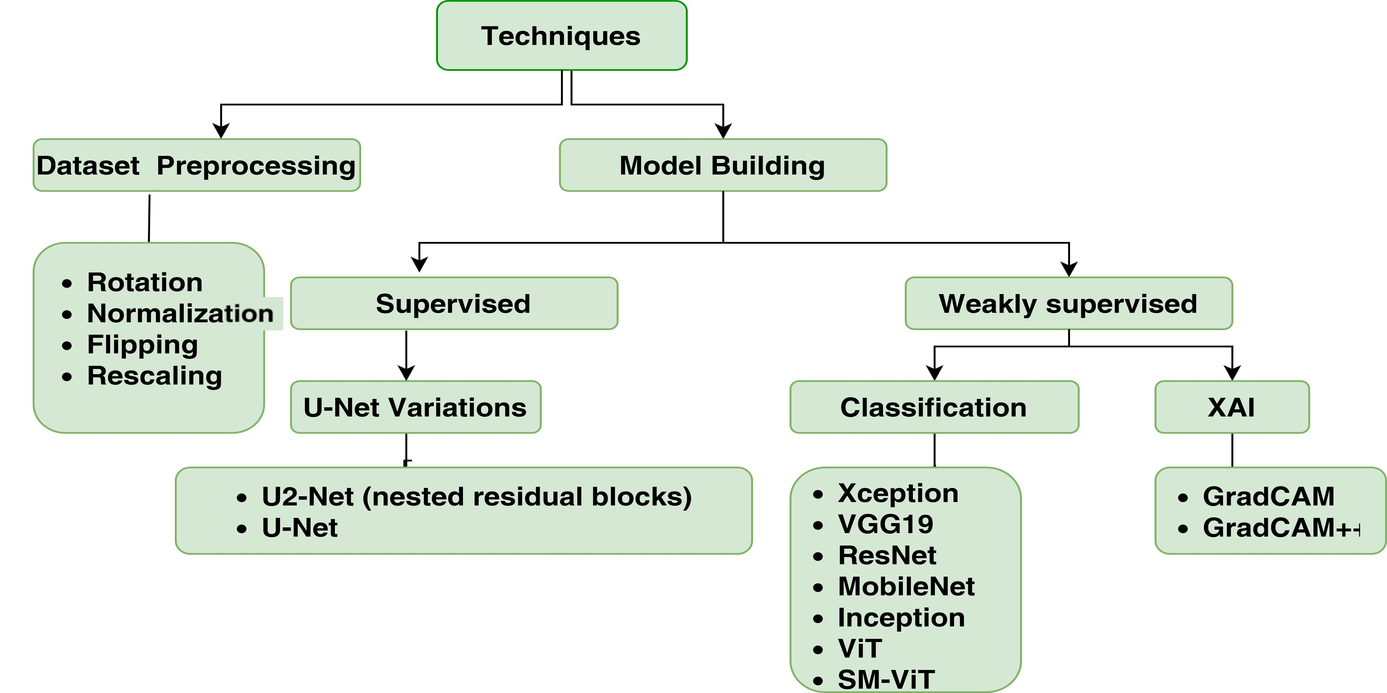In contrast, ViT models rely on self-attention mechanisms, where each input patch attends to all other patches, allowing for the modeling of long-range dependencies and capturing global context information [10,21]. The DL approaches and techniques considered for this study are shown in Figure 1 and Figure 2 shows the high-level view of the process.

The model is trained using the HAM10000 [6]. In the ViT-based approach, a mask-guided ViT is used for the segmentation as a novel contribution. In order to perform the explainability, ISIC 2018 task 2 dataset is used as it has attribute masks to evaluate the Grad-CAM and Grad-CAM++ heat maps. We employed a mask-guided approach, leveraging ViT technology to enhance self-attention mechanisms for the precise identification of melanoma skin cancer. Our strategy involved integrating U2-Net-generated masks alongside traditional self-attention mechanisms. In the context of CNN models, we also applied a masked-guided technique to curate datasets, effectively eliminating extraneous regions from skin images, thereby improving the accuracy of our skin cancer detection system. This innovative approach allowed us to focus attention where it matters most, ultimately enhancing the diagnostic capabilities of our model.

3.2. Dataset

This study uses a widely used public dataset for melanoma identification, the HAM10000 dataset [6], which contains over 10,000 images of skin lesions, including Nevi and malignant melanoma. Each image is accompanied by clinical metadata, including diagnosis, age, and sex. This dataset contains 7 categories of skin lesions. Nevus lesions [Nevi] (6705), dermatofibroma (115), malignant skin tumors [Melanoma] (1113), benign keratosis (1099), basal cell carcinoma (514), actinic keratosis (327), and vascular lesions (142) are those categories. Figure 3 shows a sample image from each class in HAM10000 dataset. We observed that certain images share identical HAM IDs, and their lesion structures exhibit congruence, leading to duplicate data. Therefore, we performed a comprehensive comparative study with the entire dataset as well as removing the duplicate images in the original dataset. We extracted 614 nevus or Nevi images (not cancer) and 614 malignant melanoma lesion images (skin tumors), which is a particularly challenging clinical task by removing any duplicates [17]. That dataset was used to feed the U2-Net [22] model and obtained the segmentation masks. This HAM10000 dataset is used to train our CNN-based models and ViT base model.

The International Skin Imaging Collaboration (ISIC) has released several public datasets for melanoma identification. We also used the ISIC 2018 task 2 dataset [23] to evaluate our explainability methods, as it contains attribute masks. This dataset contains 2594 images and 12,970 corresponding ground truth response masks (5 for each image). Those dermoscopic attribute masks contain dermoscopic attributes such as pigment network, negative network, streaks, milia-like cysts, and globules, as shown in Figure 4. Furthermore, we used ISIC 2017 dataset [23] to generate the correct segmentation mask corresponding to image lesions by training the U2-Net model. Figure 5 shows the sample image and its segmentation mask in the ISIC 2017 dataset.

3.3. U2-Net Based Segmentation Model

The U2-Net model was proposed by Qin et al. [22], which is a deep nested U-structure for salient object detection (SOD). The U2-Net architecture exhibits a two-level nested U-structure, which captures contextual information at varying scales by leveraging the fusion of receptive fields with different sizes within the residual U-blocks (RSU) architecture. Thus, the model captures more fine-grained details and produces accurate segmentation masks. It is specifically designed to separate the foreground object from the background in an image. This mechanism enables the model to encode a comprehensive understanding of the image content. Moreover, the U2-Net architecture achieves increased depth while minimizing the computational cost by incorporating pooling operations within the RSU blocks. This design choice enhances the model’s capacity without imposing a significant computational burden. Notably, the U2-Net architecture stands out by enabling end-to-end training without relying on pre-trained backbones from image classification. This model has shown competitive performance in both qualitative and quantitative evaluations [24].

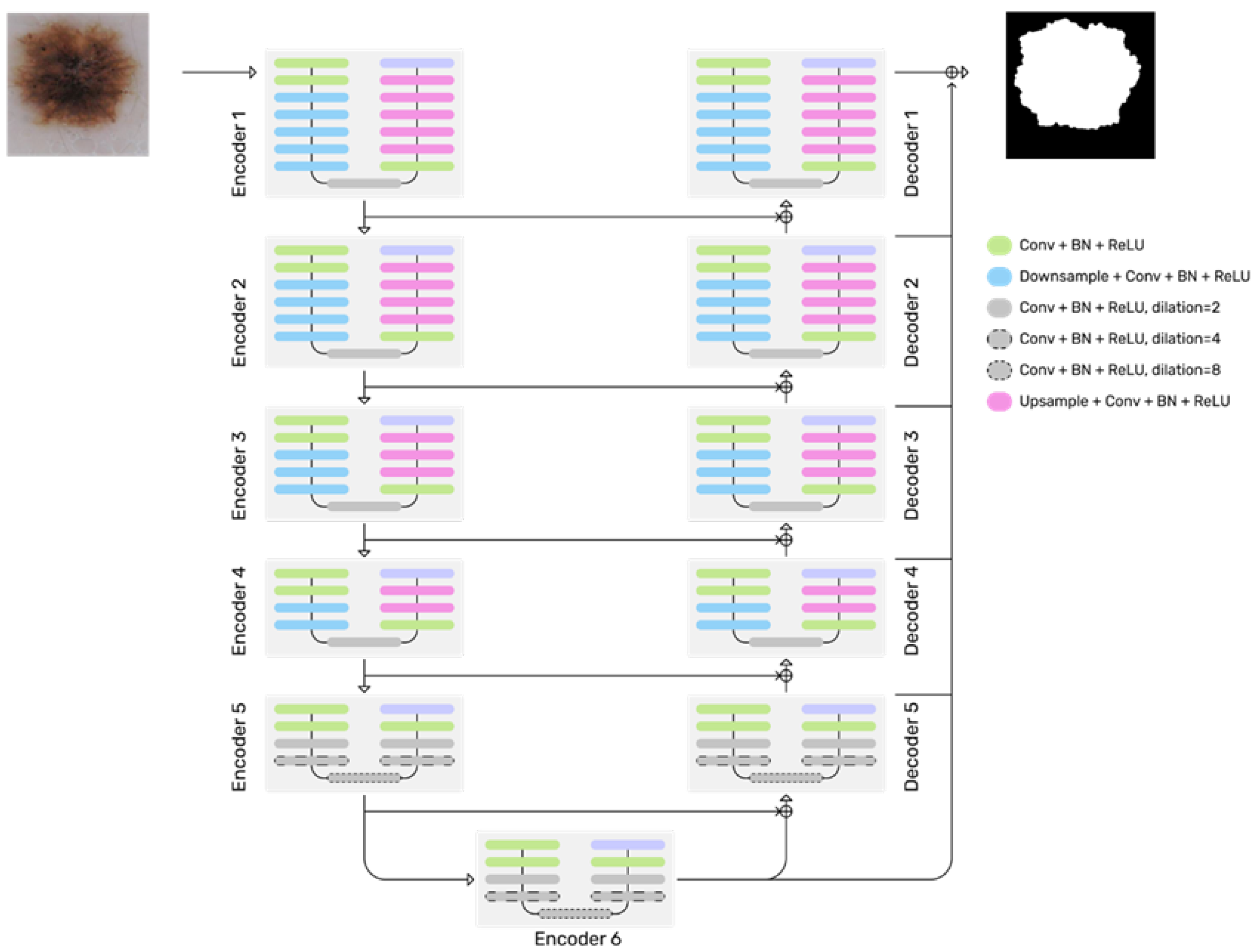
U2-Net is a two-level nested U-structure, as shown in Figure 6. Its top level is a big U-structure consisting of 11 stages. Each stage consists of a well-configured RSU (bottom-level U-structure). Hence, the nested U-structure enables the extraction of intra-stage multi-scale features and aggregation of inter-stage multi-level features more efficiently. The U2-Net mainly consists of three parts: (1) six-stage encoder, (2) five-stage decoder, and (3) saliency map fusion module attached to the decoder stages and the last encoder stage.

The U2-Net architecture uses RSUs of varying heights, (L) in its encoder stages (En) to capture different scales of information in the input feature maps. The En5 and En6 stages use dilated versions of the RSU-4 block to avoid further down-sampling of the low-resolution feature maps. The decoder stages (De) have similar structures to their corresponding encoder stages, with De5 using the dilated RSU-4F block. The saliency map fusion module generates saliency probability maps by first generating six side output saliency probability maps from different stages of the network and then upsampling and fusing them with a concatenation operation followed by a 1 × 1 convolution layer and Sigmoid function to generate the final saliency probability map. The corresponding pseudocode is given in Algorithm 1. Accordingly, the generated masks from the segmentation process are used for the classification pipelines.

Algorithm 1: Proposed segmentation module training pipeline

3.4. CNN-Based Classification

We performed a comparative study utilizing different CNN-based models and with two different variations in the HAM10000 dataset. Initially, we tried with all the melanoma and Nevi lesion images in the dataset. Since, there are duplicate images, we removed the duplication of melanoma images and Nevi images to maintain the class balance between melanoma and Nevi lesion images from the dataset. Next, we obtained all melanoma images and the same number of Nevi images from the non-duplication image set and then we split it into training, validation, and testing according to 80:10:10 ratio.

Table 1. Image count before and after removing duplication.

	Melanoma	Nevus Lesions [Nevi]
Before removing duplication	1113	6705
After removing duplication	614	5404
Balanced image count	614	614

shows the image count of before and after removing duplicates.

Table 2. Image counts originally considered for data split.

Skin Cancer	Training Set	Testing Set	Validation Set
Melanoma	512	65	64
Nevus	512	65	64

summarizes the number of original images used for the training, testing and validation datasets.

Next, we applied two pipelines. As the first pipeline, we incorporated the U2-Net model to generate segmentation masks of the raw images and apply those masks to the original image (mask-guided experiment). The second pipeline is performed without applying segmentation masks to the original images (non-mask-guided experiment). In order to use the U2-Net model, we have used a pre-trained U2-Net model, which is trained with ISIC 2017 challenge datasets. It contains lesion segmentation data, including the original image, paired with the expert manual tracing of the lesion boundaries in the form of a binary mask. We used these binary images as the label for each image and used “epoch_num = 20 batch_size_train = 32 batch_size_val = 1” parameters for the training. After generating segmentation masks using the trained U2-Net model, we applied those masks to the respective images. A sample image input and generated masks after going through the U2-Net model are shown in Figure 6, as the input and output images. Figure 7 shows a sample image input, generated masks from the U2-Net model, and an image obtained after applying the segmentation mask.

In DL model training, it is important to have a balanced image count in each of the classes in the dataset that is considered for model building. Having equally represented classes helps to avoid biased predictions, improves the generalizability for unseen data, stable model training, effective pattern learning, and supports reliable evaluation. Data imbalance issues can be addressed by data augmentation or a specially designed loss function, based on the nature of the dataset. Data augmentation techniques help to increase the number of data records in each class and have a balanced dataset. Different transformations can be applied to increase the diversity of the training data, which supports regularization and generalization. This leads to preventing overfitting and obtaining a robust model for input variations. Moreover, when there is a limited amount of training data, data augmentation helps the model to improve feature learning and extract more meaningful and generalized features; thus, improves the model performance.

As the next step, we applied augmentation operations, such as flipping, rotation, and rescaling. The aforementioned augmentations were selected based on their ability to preserve the structural integrity of the lesions during the training process. It was imperative to avoid cropping and shifting operations that could potentially compromise the lesion structure, leading to erroneous training outcomes. By employing the chosen augmentations, we aimed to mitigate the risk of introducing distortions that could negatively impact the accuracy and reliability of the training procedure. We resize all images into 224 × 224 scale, to ease the training process. In our second experiment, we followed all the above processes except mask generating and applying masks stages.

Subsequent to the aforementioned pre-processing steps, the dataset was utilized within the framework of a CNN model. The adoption of the transfer learning technique supported to obtain high results with the limited size of the dataset [21]. In order to leverage the knowledge gained from larger datasets, we employed pre-trained models, specifically Xception [25], ResNet50 [26], VGG16 [27], InceptionV3 [3], and MobileNet [20]. These models were subjected to extensive experimentation to achieve optimized and accurate results. All base models are pre-trained using the ImageNet dataset, which contains a large number of annotated images belonging to objects in the world.

In our comparative study, we experimented with the original models as well as modifying the CNN architectures to obtain better results. This helps to justify the architectural changes we proposed in this study provides better results than the base models. The experiments were performed for both mask-guided and non-mask-guided pipelines.

We modified the original base model by adding a global average pooling layer (GAP), a dense layer, and a dropout layer. The GAP layer supports the implementation of the explainability approaches. Moreover, we applied regularization methods, such as early stopping callbacks, to avoid overfitting the model. This study utilized the Bayesian hyperparameter tuner [28], to train our CNN models, facilitating the discovery of optimized parameters and resulting in optimized models. The considered parameter ranges are presented in

Table 3. Considered hyperparameter ranges.

Parameter Name	Range
Epochs	1–100
Number of search rounds	4
Number of iterations per search	3
Learning rate	0.0000001–0.0001
Number of nodes in the Dense layer	50–255
Dropout	0.1–0.8
Optimizer function	Adam/SGD

. This hyperparameter tuning supports in refining the performance of CNN models by systematically exploring the parameter space and identifying the configurations that yield superior results. Furthermore, we retrained only some of the lower batch-normalization layers by unfreezing from its base model, during the training process.

We identified the high-performing models using the Bayesian hyperparameter tuner.

Table 4. Used hyperparameters for the top models.

Parameter Name	Xception	ResNet50	VGG16
Epochs	92	60	73
Number of searches	4	4	4
Number of iterations per search	3	3	3
Learning rate	1.7 × 10−5	1.3 × 10−4	5.5 × 10−6
Number of nodes in the dense layer	103	171	204
Dropout	0.741	0.553	0.563
Optimizer function	Adam	Adam	Adam

shows the hyperparameters used for those top models, namely, Xception, ResNet50, and VGG16. Moreover, the supplementary results of the mask-guided technique, without eliminating the duplicates are presented in Section 4 and have shown that the models trained without duplicate images have given high results. Furthermore, our explainability methods were employed on the trained models subsequent to the optimization process. We applied XAI techniques only for the models with high performance. In this case, models obtained from mask-guided experiments are used for explainability methods, as described in Section 3.6. This section elucidated the techniques and approaches employed to gain insights into the decision-making processes of the trained models. The above mentioned process is stated in Algorithm 2.

Algorithm 2: Proposed CNN-based classification and explainability pipeline

3.5. ViT-Based Classification

The ViT architecture, initially designed for less fine-grained problems, is supposed to capture both global and local information, which makes it spend a noticeable part of its attention performance on the background patches [10,21,29]. This property makes vanilla ViT perform worse on FGVC tasks, since they usually require finding the most distinguishable patches, which are mostly the foreground ones. In order to resolve this issue, we used salient mask-guided vision transformer (SM-ViT), which embedded information from a saliency detector into the self-attention mechanism. The overall architecture of our SM-ViT is illustrated in Figure 8.

In the proposed design, we used the ViT model as the backbone for the classification. Here, a ViT B/16 model pre-trained on the ImageNet-21K dataset [30], with 224 × 224 images and with no overlapping patches. For the saliency detection module, a U2-Net model pre-trained on the ISIC 2017 Task 1 dataset, is used with constant weights. Following common data augmentation techniques, unless stated otherwise, the image processing procedure is as follows: for the saliency module, as recommended by the authors [22], the input images are resized to 320 × 320, and no other augmentations are applied. The pseudocode of the ViT-based classification is shown in Algorithm 3.

For our SM-ViT, the images are resized to 224 × 224 for the HAM1000 dataset. Next, random horizontal flipping and color jittering techniques are applied only for the training process. All our models are trained with the standard SGD (stochastic gradient descent) optimizer with a momentum set to 0.9 and with a learning rate of 0.03, all with cosine annealing for the optimizer scheduler. The batch size is set to 32 for all datasets. Pre-trained with 224 × 224 images, ViTB/16 weights are loaded from the original ViT [10] resources.

Initially, we utilize a salient object detection (SOD) module for saliency extraction. Our method employs a popular deep saliency model, U2-Net pre-trained on a mid-scale dataset for salient object detection. Here, the nested U-shaped architecture predicts saliency based on rich multi-scale features at relatively low computation and memory costs. First, an input image is passed through the SOD module set up in a test mode, which further generates the final non-binary saliency probability map. In the next phase, the model output is normalized to be within the values [0…1] and then converted into a binary mask by applying a threshold dα on each mask’s pixel, where dα is a pixel’s intensity threshold. We used a threshold of 0.8 [22]. Finally, the resulting binary mask and a bounding box for the found salient object(s) (in the form of the minimum and maximum 2D coordinates of the positively thresholded pixels) are extracted and saved.

Algorithm 3: Proposed ViT-based classification and explainability pipeline

An important note is that our solution also takes into account the cases when a mask is not found or is corrupted, and, if so, the initial probability map is first refined again using a threshold dα = 0.2, which allows more pixels to be considered positive. If the mask is not restored even after refining, its values are automatically set as positive for the central 80% of the image pixels. The extracted binary mask and bounding box are further passed into our SMGE. The core module of SM-ViT is our novel salient mask-guided encoder (SMGE), which is a ViT-like encoder modified to be able to receive and process saliency information. Its main purpose is to increase the class token attention scores for the image tokens containing foreground regions. Initially, an image, cropped according to the extracted in the SOD module bounding box, in the form of patches is projected into linear embeddings, and a position embedding is added to it. Next, instead of the standard ViT encoder, our SMGE takes its place functioning as an improved self-attention mechanism.

$$Attention\left(Q,K,V\right)=softmax(\frac{Q{K}^T}{\sqrt{d_k}})V$$

(1)

In order to understand the intuition behind our idea, we need to emphasize that the manner in which attention is obtained in the vanilla ViT encoder (Equation (1)) makes the background and foreground patches equally important and does not discriminate valuable for FGVC problems salient regions of the main object(s) in an image. Taking this issue into account, our solution is to increase attention scores for the patches that include a part of the main (salient) object in them. However, due to the nature of the self-attention mechanism and the non-linearity used in it, one can not simply increase the final attention values themselves since it will break the major assumptions of the algorithm [10]. Therefore, we modified the attention scores calculated before the soft argmax function (also known as softmax), according to the saliency mask provided by the salient object detection module. For this purpose, the binary mask is first flattened into a 1D vector and a value for the class token is prepended to it, therefore that, similar to Equation (1), the size of the resulting mask matches the number of tokens (Np + 1), as in Equation (2), where $m_{cls}$ is always positive since the attention of the class token to itself is considered favorable. Further, a conventional attention score matrix $X^{scor}$ is calculated in each head as in Equation (3).

$$m=\left[m_{cls};m_p^1;m_p^2;m_p^3;\dots .;m_p^{N^p}\right]$$

(2)

$$X_{scor}=\frac{Q{K}^T}{\sqrt{d^k}}V$$

(3)

Next, the maximum value $X_{max}$ among the attention scores of the class token to each patch is found for each head. These values are further used to modify the attention scores of the class token by increasing the unmasked by m ones with a portion of the largest found value $X_{max}$, which is calculated for every head. $X_{scor\left(cls\right)}$ is a row in the matrix of attention scores $X_{scor}$ belonging to the class token, $d_{\theta }$ is a coefficient controlling the portion of the maximum value to be added, and $iϵ\left[1,2,\dots ,N_P,N_{P+1}\right]$. Finally, as in Equation (4), the rows of the resulting attention score matrix $X_{scor}$, including the modified values in its $X_{scor\left(cls\right)}$ row, are converted into probability distributions using a nonlinear function.

$$Y=softmax\left(X_{scor}\right)$$

(4)

Eventually, similar to the multi-layer vanilla ViT encoder, the presented algorithm is further repeated at each SMGE’s layer until the classification head, where the standard final categorization is performed based on the class token aggregating the information from the “highlighted” regions throughout SMGE. To summarize, our simple yet efficient salient mask-guided encoder changes the vanilla ViT encoder by modifying its standard attention mechanism’s algorithm (in Equation (1)) with Equations (2)–(4). Therefore, relative to the vanilla ViT encoder, our SMGE only adds pure mathematical steps, does not require extra training parameters, and is not resource-costly.

3.6. Explainability

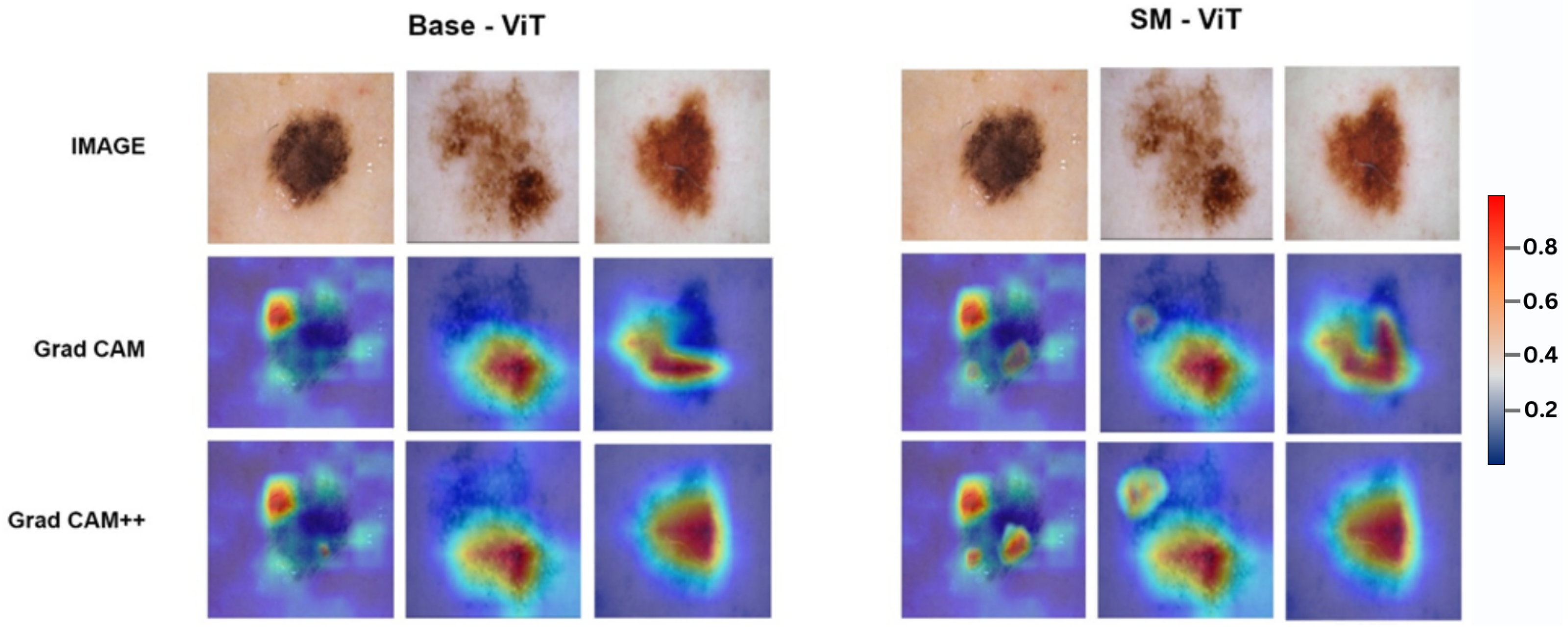
With the increasing development of real-world applications using DL models, it is important to build trust and transparency of the results to the user. XAI techniques support understanding the regions-of-interests of the input that cause to predict the results. In this study, we applied both Grad-CAM and Grad-CAM++, as novel contributions to the domain of dermatology. It helps to identify the gradient of the most dominant feature maps of the final convolution layer in the trained model as the explainability approach of the solution [21]. Here, we applied the XAI techniques only for the mask-guided models presented in this study, which are identified as high-performance models.

The CAM, Grad-CAM, and Grad-CAM++ are considered as the series of CAM explainability techniques. The explainability prowess of the CAM is limited to only CNNs, which have GAP at the penultimate layer, which is a fully connected hidden layer. Furthermore, CAM requires retraining multiple linear classifiers after training the base model. The Grad-CAM technique addresses this issue by introducing a backpropagation concept. It also considers a GAP of the partial derivatives to solve the weight independent from the position of a particular activation map. Even though Grad-CAM is better than CAM, Grad-CAM heatmaps cannot localize the entire region of the object. Grad-CAM++ is used to address this using a weighted combination of the positive partial derivatives of the last convolutional layer feature maps. Compared to Grad-CAM, the Grad-CAM++ technique gives more highlighted heatmaps even though related features are bounded to a limited pixel area [8].

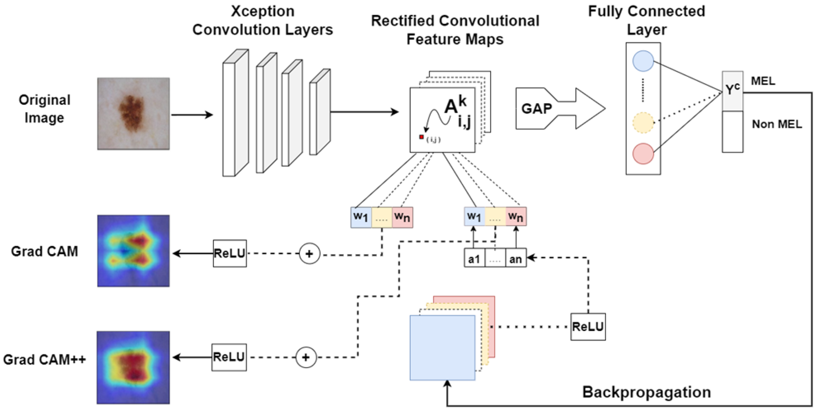
The explainability model consists of a series of convolutional layers, rectified convolutional feature maps, and fully connected layers, as shown in Figure 9. After the last convolution layer, we applied the GAP for all feature maps to obtain a single scalar for each map. The class scores for a given class are found using the combination of those single scores of each activation map with the multiplication of the weights at the fully connected layer. Consequently, in the Grad-CAM, backpropagation is applied until the last convolution layer to find the weights for each feature map using the global average pool of the partial derivative. We applied the ReLu activation function to combine the positive partial derivatives of the final convolutional layer feature maps corresponding to a particular class score as gradient weights to produce visual explanations of the model predictions, considering the object localization [8]. Subsequently, the linear combination of the derived weights is added through the ReLu activation to obtain positive correlations and generate the Grad-CAM heatmap.

Moreover, we applied Grad-CAM++ as a comparison study. Here, a similar backpropagation is applied until the last convolution layer to find the weights, which are derived by taking the positive partial derivatives w.r.t each feature maps using the ReLu activation function and multiplying by pixel-wise weight $\alpha$. Finally, the model uses ReLu to obtain the heatmap visualization as of the Grad-CAM. In this process, for a particular skin image, the CNN model first extracts the convolutional feature maps $A^k$. The final score $Y^c$ for a particular class c, is expressed as a linear combination of its global average pooled final convolutional layer feature maps using Equation (5) [8]. Here, $w_k^c$ is the weight for a particular feature map $A^k$ of class c, as given in Equation (6). It is the positive gradient weighted average of the gradients with positive partial derivatives w.r.t. each pixel in an activation map $A^k$, $\frac{\partial Y^c}{\partial A_{i,j}^k}$ with the ReLu function ([8]). The pixel-wise weights ${\alpha }_{i,j}^{kc}$ for a specific class c and the locations (i, j) of a specific activation map k are determined as stated in Equation (7). Here, the activation map $A^k$ is iterated over by (i, j) and (a, b).

$$Y^c=\sum _k^{ }{w}_k^c.\sum _i^{ }\sum _j^{ }{A}_{i,j}^k$$

(5)

$$w_k^c=\sum _i^{ }\sum _j^{ }{\alpha }_{i,j}^{kc}.relu(\frac{\partial Y^c}{\partial A_{i,j}^k})$$

(6)

$${\alpha }_{i,j}^{kc}=\frac{\frac{{\partial }^2{Y}^c}{{(\partial A_{i,j}^k)}^2}}{2\frac{{\partial }^2{Y}^c}{{(\partial A_{i,j}^k)}^2}+{\sum }_a^{ }{\sum }_b^{ }{A}_{ab}^k\frac{{\partial }^3{Y}^c}{{(\partial A_{i,j}^k)}^3}}$$

(7)

3.7. Implementation Details

Overall architecture with salient object detection (SOD) module and salient mask-guided encoder (SMGE) have been implemented and currently optimizing the parameter to improve the accuracy. All our experiments are conducted on a single NVIDIA RTX 2000 GPU using the PyTorch deep learning framework and the APEX utility, and all the results are stated. The used DL platforms, libraries and tools are as follows.

• TensorFlow: provides the core framework for building and training DL models. We used these libraries to implement the CNNs for classifying melanoma skin cancer images;
• Keras: simplifies the process of building and training these models and places as a high-level API built on top of TensorFlow. We used CNN architectures such as ResNet50, VGG16, and Xception, which can be conveniently implemented in Keras with pre-trained weights, facilitating transfer learning;
• PyTorch: as another widely used framework for building and training DL model and supports tasks, such as data loading and pre-processing, model training, and implementing model architecture. The associated dynamic computational graph and efficient memory usage, enables large-scale DL tasks. We have used this library to develop ViT based approach;
• Scikit-learn (sklearn): is a Python library that supports classification tasks and interoperates with the Python numerical and scientific libraries NumPy and SciPy. We used Scikit-learn during the model evaluation process;
• NumPy: is a Python library that supports large scale, multi-dimensional arrays and matrices. This enables high-level mathematical functions to operate on these arrays. We used NumPy for numerical operations, manipulating arrays for data preprocessing, and integration with other libraries like TensorFlow and PyTorch;
• Matplotlib: is a plotting library in Python and its numerical mathematics extension NumPy. It provides an object-oriented API for embedding plots into applications using general-purpose GUI toolkits. We used Matplotlib for visualizing data, plotting the training history of models, or displaying the heatmaps generated by Grad-CAM and Grad-CAM++.

4. Result and Discussion

4.1. Segmentation Result

To give an intuitive understanding of the promising performance of the U2-Net model, Figure 10 shows sample segmentation results of U2-Net and U-Net models.

As we can observe, U2-Net can produce more accurate results on both small and large objects compared to U-Net, whose models are either prone to miss the small target or produce large objects with poor accuracy. Thus, U2-Net can handle different types of targets and produce more accurate salient object detection results than U-Net. The outputs of the deep salient object methods are usually probability maps that have the same spatial resolution as the input images. Each pixel of the predicted saliency maps has a value within the range of 0–1 (or [0, 255]). The ground truths are usually binary masks, in which each pixel is either 0 or 1 (or between 0 and 255), where 0 indicates the background pixels and 1 indicates the foreground salient object pixels.

Table 5. Quantitative performance of the U2-Net and U- Net models.

Model	IoU	Loss	Recall
U2-Net	0.93	11.65%	92.77%
U-Net	0.84	15.40%	85.21%

shows the quantitative results of the U2-Net and U- Net models with the HAM10000 dataset. The U2-Net model achieved an IoU of 0.93, which is higher than the IoU of 0.84 achieved by the U-Net model. This indicates that the U2-Net model performed better in terms of accurately segmenting the images. Loss is a metric used to measure the difference between the predicted output and the ground truth. Lower loss values indicate better performance. The U2-Net model achieved a lower loss of 11.65% compared to the U-Net model’s loss of 15.40%. This indicates that the U2-Net model had better overall performance and achieved a better fit to the training data. Recall measures the proportion of actual positives that are correctly identified by the model. Higher recall values indicate better performance. The U2-Net model achieved a higher recall of 92.77% compared to the U-Net model’s recall of 85.21%. This indicates that the U2-Net model was better at correctly identifying positive cases in the images.

4.2. Classification Result

4.2.1. Results of CNN Classification

We have evaluated each of the models from different perspectives. Accuracy is the most common metric used to evaluate deep learning models. It measures the proportion of correct predictions made by the model overall predictions made. Specificity is the ability to designate an individual who does not have a disease as negative. It is important in medical decisions because then patients should not go for further treatments. Sensitivity is the ability to designate an individual with a disease as positive. This helps to identify melanoma from this model. The calculation equations of each metric are given in Equations (8)–(10), where TP, TN, FP, and FN are defined as follows:

TP (true positives) = Number of samples correctly classified as melanoma;

TN (true negatives) = Number of samples correctly classified as nevus;

FP (false positives) = Number of samples incorrectly classified as melanoma;

FN (false negatives) = Number of samples incorrectly classified as nevus.

$$Accuracy=\frac{TP+TN}{TP+TN+FP+FN}$$

(8)

$$Sensitivity=\frac{TP}{TP+FN}$$

(9)

$$Specificity=\frac{TN}{TN+FP}$$

(10)

Table 6. Performance metrics of CNNs for mask-guided experiments (Highest values are indicated in bold font).

Model	Accuracy	Sensitivity	Specificity
Xception *	98.37%	95.92%	99.01%
Vanilla-Xception	84.55%	89.79%	81.08%
ResNet50 *	98.18%	97.95%	98.65%
Vanilla-ResNet50	86.91%	91.83%	83.78%
VGG16 *	97.56%	97.82%	97.40%
Vanilla-VGG16	80.13%	86.54%	79.83%
Inception *	95.93%	91.83%	98.64%
Inception	61.78%	99.9%	36.48%
MobileNet *	96.56%	93.87%	98.99%
MobileNet	95.93%	89.79%	97.89%

* denotes modified CNN models.

presents the performance values obtained for different CNN models with respect to mask-guided experiments for the dataset that has removed the duplicate images. A comparative study of the results is shown between the original models and the modified models, which have included a GAP layer, a dense layer, and a dropout layer, as explained in Section 3.4. Notably, our modified Xception model demonstrates the highest accuracy of 98.37%. Moreover, the specificity metric, which measures the ability to identify nevus instances correctly, achieves an impressive value of 99.01% for the modified Xception model. On the other hand, the modified ResNet50 model exhibits the highest sensitivity of 97.95%, reflecting its proficiency in correctly identifying positive instances; furthermore, Inception and MobileNet results are mentioned in Table 6. These findings underscore the effectiveness of our modified CNN models in achieving high accuracy across different evaluation metrics.

Table 7. Performance metrics of CNNs for non-mask-guided experiments.

Model	Accuracy	Sensitivity	Specificity
Xception *	90.94%	91.83%	89.18%
Xception	82.11%	95.92%	72.97%
ResNet50 *	91.05%	99.90%	85.13%
ResNet50	88.61%	93.87%	85.13%
VGG16 *	93.49%	91.83%	94.45%
VGG16	85.88%	88.12%	93.12%
Inspection *	92.68%	97.95%	89.18%
Inspection	84.55%	87.75%	82.43%
MobileNet *	91.05%	95.91%	87.83%
MobileNet	88.61%	93.87%	85.13%

* denotes modified CNN models.

states the result obtained for the non-mask-guided experiments, for the dataset that has removed the duplicate images. Here, we used the same modified and non-modified CNN models with non-mask-guided images. Here, the modified VGG16 model has shown the highest accuracy from other CNN models and its accuracy is 93.49%. Furthermore, the ResNet50 model has given the highest sensitivity as 99.90%. VGG16 model has given the highest specificity value and it is 94.45%; however, it can be observed that the results of the non-mask-guided approach are lower than the mask-guided approach shown in Table 6.

Moreover, we have performed experiments with the entire dataset, without removing any duplicate images. We have selected the mask-guided approach, as it shows better results.

Table 8. Performance metrics of CNNs for mask-guided experiments with image duplication.

Model	Accuracy	Sensitivity	Specificity
Xception *	81.17%	86.09%	75.93%
ResNet50 *	83.41%	88.70%	77.78%
VGG16 *	82.96%	91.03%	74.07%
Inspection *	79.82%	91.30%	71.30%
MobileNet *	81.16%	95.52%	64.81%

* denotes modified CNN models.

states the outcomes derived from applying modified CNN models to a dataset containing duplicated instances. Here, the modified ResNet50 model achieved the highest level of accuracy (83.41%) within this context. However, it is worth emphasizing that this performance did not surpass the results obtained when employing modified CNN models with duplicate removal (i.e., Table 6 and Table 7). In summary, it becomes evident that the presence of duplicated images has a detrimental impact on model performance.

Moreover, Figure 11 shows the confusion matrix of our modified CNN models in mask-guided experiments that have obtained the highest values in each model type. Furthermore, Figure 12 shows learning curves for those CNN-based models, and learning curves indicate that our modified CNN models have not overfitted.

Generally, AUC represents the model’s overall performance in distinguishing between positive and negative classes, typically represented as diseased versus non-diseased [21]. We obtained the receiver operating characteristic (ROC) curves and calculated AUC values. Figure 13 shows a combination graph of each ROC curve of the highest-performed models, namely, Xception, ResNet50, and VGG16. Many of the AUC values are close to one, and then we can conclude that the model has a high predictive power and performs very well in distinguishing between positive and negative instances.

4.2.2. Results of ViT Classification

Table 9. Performance metrics of ViT models.

Model	Accuracy	Sensitivity	Specificity
Base-ViT	84.68%	83.87%	85.48%
SM-ViT	92.79%	91.09%	93.54%

presents a comparative analysis of the performance metrics of the base-ViT and the proposed SM-ViT models. We can observe that the proposed SM-ViT model exhibits substantial enhancements across multiple evaluation metrics. Specifically, our SM-ViT model shows an accuracy of 92.79%, outperforming the baseline ViT model’s accuracy of 84.68%. Similarly, the sensitivity of the SM-ViT model reaches 91.09%, surpassing the baseline ViT model’s sensitivity of 83.87%. Moreover, our proposed SM-ViT model achieves a specificity of 93.54%, displaying a remarkable improvement over the baseline ViT model’s specificity of 85.48%. These results affirm the performance improvements of our SM-ViT model when compared to the baseline ViT model, highlighting its effectiveness in accurately classifying melanoma and underscoring its potential for enhancing medical image identification tasks. Moreover, Figure 14 shows the confusion matrix of ViT-based models. Both the SM-ViT and Baseline ViT models have demonstrated higher accuracy in identifying Nevi lesions compared to melanoma. Therefore, both models exhibit good sensitivity when it comes to Nevi detection.

4.3. Explainability Results

4.3.1. Overall Explainability

We generated heatmaps for the images utilizing XAI techniques, namely, Grad-CAM and Grad-CAM++. Figure 15 gives an overall comparison of results obtained by the two methods. The evaluation of the explainable approaches is presented both quantitatively and qualitatively. We considered the gradients of the most dominant logit corresponding to the feature maps of the final convolution layer. Thereby, we identified the positions of the features of the image that are considered by the model for the predictions.

We evaluated the performance of our model against ground truth and generated maps using the ISIC 2017 binary mask dataset and ISIC 2018 attribute mask dataset. The metric IoU is used for the quantitative evaluation. For the qualitative evaluation, a comparison of the Grad-CAM and Grad-CAM++ visualization for a given image is shown in Figure 15. The color range in the explainable heatmap indicates the regions that have contributed more and less to the classification, using red and blue, respectively. The attribute masks corresponding to each image are also used to validate the explanations by comparing them with the predicted heatmap outputs. Accordingly, Grad-CAM++ shows better explainability than Grad-CAM, with more region coverage provided by the attribute masks.

Here, we selected the ISIC 1017 dataset for quantitative evaluation, because it has binary masks that can be used to find bounding box annotations for each of its images. The IoU metric $Lo{c}_I^c$, for a particular class c, threshold value δ, and an image I, is calculated as in Equation (11). Here, Area(bounding box) refers to the area of the bounding box/es for a particular class c and a given image I, Area(internal pixels) denotes the number of non-zero pixels in the explanation map that lie inside the bounding box/es, and Area(external pixels) states the number of non-zero pixels that lie outside the bounding box/es. The higher the value of Loc, the better the localization of the explanation map. Moreover, Figure 16 shows visual examples of the improved object localization obtained by the proposed method.

$$LO{C}_C^I\left(\delta \right)=\frac{Area(Internal pixels)}{Area(bounding box)+Area(external pixels)}$$

(11)

4.3.2. Explainability of CNN Based Models

We applied the XAI techniques for each CNN model separately and compared the results of the heat maps. Note that, as given in Table 6, the Xception model has shown the highest accuracy and specificity for the mask-guided approach, and the ResNet50 and VGG16 models have also shown better results among others. Therefore, we applied the XAI techniques for those models with high performance metric values.

A set of sample images used for the explainability process with the selected models is shown in Figure 17. The first row of images corresponds to skin-related images, while the second and third rows display images relevant to specific Grad-CAM and Grad-CAM++ explainability methods. Notably, our findings indicate that the Xception model outperformed the other two CNN models in terms of explainability. This insight plays a pivotal role in enhancing the model’s trustworthiness by visually demonstrating the areas within an image that contributed to its classification.

Furthermore, we use IoU to evaluate the quantitative effectiveness of Grad-CAM, and Grad-CAM++ for class-discriminative localization of objects in a given image. The obtained results are shown in

Table 10. Average IoU values for the explainability of CNN models.

Model	Average IoU (Grad-CAM++)	Average IoU (Grad-CAM)
ResNet50 *	0.5093	0.4932
Xception *	0.4745	0.4664
VGG16 *	0.3968	0.3981

* denotes modified CNN models.

. We note that the same was used to threshold both explanation maps (Grad-CAM++ and Grad-CAM) for fairness of comparison w.r.t each CNN model.

4.3.3. Explainability of ViT-Based Models

We apply the expandability method for Base-ViT and SM-ViT models separately and compare the heat maps results. Figure 18 shows a set of different images with the corresponding Grad-CAM and Grad-CAM++ visualizations. It can be seen that Grad-CAM++ provides better explanations compared to the Grad-CAM technique. Furthermore, according to these results, the SM-ViT model provides a better explanation than other models.

Here also, IoU is used to evaluate the quantitative effectiveness of Grad-CAM, and Grad-CAM++ for class-discriminative localization of objects in a given image as used with CNN model. The results are stated in

Table 11. Average IoU values for the explainability of each ViT model.

Model	Average IoU (Grad-CAM++)	Average IoU (Grad-CAM)
Base-ViT	0.5463	0.5822
SM-ViT	0.6220	0.6947

. We note that the same was used to threshold both explanation maps (Grad-CAM++ and Grad-CAM) for fairness of comparison w.r.t each ViT model.

Furthermore, Figure 19 displays a comparison of the IOU values obtained from the Grad-CAM and Grad-CAM++ heat maps for each model. Accordingly, the VGG16 model exhibits the lowest IOU values, indicating a relatively weaker alignment between the heat maps and ground truth annotations. Conversely, the SM-VIT model demonstrates the highest IOU values for both Grad-CAM and Grad-CAM++, underscoring its superior alignment and closer correspondence with the ground truth annotations.

5. Results Validation and System Usability

5.1. Web Application Support Solution

We have deployed the proposed model as a support tool named LU Bio Vision and a sample GUI is shown in Figure 20. The web application provides a user-friendly interface to test a skin image for melanoma conditions. Our implementation based on the segmentation followed by the classification model, which is integrated with the XAI techniques, is built in GitHub (https://github.com/LU-Bio-Vision, accessed on 30 January 2024) and GoogleCloud is used to deploy the web application.

The application allows to upload a skin image. An image editor is available in the user interface to edit the image before sending it to the prediction model. Here, the user can select the proposed CNN model or the ViT-based model to classify the image. Then the system generates the corresponding heatmaps together with the predicted class with the accuracy probability. Additionally, users can generate and download the medical report in PDF format with dermatologist feedback.

This web-based solution can be used by the medical practitioners and interns as a support tool. They can get an idea about the position of melanoma attributes, the image regions that impacted for making the classification, and the details related to the decision-making process. Accordingly, this application enables the trustworthiness of the underlying DL model with explainable techniques.

5.2. Real-World Validation of Results

We conducted a study among experts in the medical domain to validate the results obtained from the proposed approach. We used 10 skin images that could belong to a person infected with melanoma or non-melanoma and obtained the domain experts’ knowledge to identify the category of each skin image. Additionally, we recorded the reasons for their decision for each image and their view on having a computational support tool to assist the melanoma diagnosis process. We selected skin images with five non-melanoma conditions and five melanoma conditions.

We have performed a survey (https://forms.gle/xz6EHTHvaqDWLfqs6, accessed on 30 January 2024) among a dermatological oncologist (skin surgeon) with 5+ years of experience, 9 doctors with 2–5 years of experience, and 11 medical interns who have 1-year experience with skin image analysis. These medical interns are practicing under senior dermatologists. The main objective of this is to check the accuracy and the time taken to make the decisions. We checked the classification accuracy of the same set of images from the automated model that we have proposed. The accuracy of the classification results provided by different user categories and the presented model is shown in Figure 21. Accordingly, the average classification accuracies shown by dermatological oncologists, doctors, and medical interns are obtained as 100%, 90.20%, and 87.5%, respectively.

It can be observed that the classification by the dermatological oncologist (skin surgeon) gives 100% accurate results and it complies with the results obtained from the proposed automated DL model, for the selected images. Thus, we can state that our model performs well and can be used in clinical practice as a support tool that gives a second opinion. We need to emphasize that this proposed solution is not a replacement for the practitioners’ decision. Considering the responses of medical interns, the results are satisfactory based on their level of experience; however, they can use this tool to verify their decisions. Therefore, this application can be mainly used by people in the field with less experience as a learning support tool that gives a second opinion for melanoma detection using skin images.

5.3. System Usability Study

We conducted another survey (https://forms.gle/n4a6aNfQYt1Ssn288, accessed on 30 January 2024) for the usability assessment of a melanoma skin cancer identification tool, specifically the web application. This standard system usability study (SUS) helps to evaluate the usability of the developed segmentation, classification, and explainability models. The SUS survey comprised 10 questionnaires that aimed to capture both positive and negative aspects of usability. Participants provided their responses on a 5-point Likert scale, ranging from “1” indicating “strongly disagree” to “5” indicating “strongly agree”. Here, the odd and even numbered questions focused on measuring positive and negative impact, respectively. The final SUS score was calculated by averaging the individual SUS scores obtained from users’ responses.

The survey was conducted among 21 medical professionals, encompassing medical interns, doctors, and dermatologists. The evaluation of our proposed system yielded an impressive average SUS score of 86.87%, indicating "excellent" usability according to the standard definition. This high score reflects the positive reception of the system by the participants. Figure 22 provides an illustrative representation of the results. Accordingly, the survey revealed that 100% of the participants found the system to be easy to use, well integrated, instilled confidence in its usage, quick to learn, and overall usable. Considering the fact that the majority of our participants are medical professionals who routinely employ various websites throughout their practice, these positive responses are well-founded.

6. Discussion

The main aim of this study was to propose a model and develop a solution for the identification of melanoma skin cancer images. We investigated the effectiveness of mask-guided DL methods for melanoma diagnosis. Two main approaches, namely, the CNN-based approach and the ViT-based approach, were explored with the HAM10000 dataset in this research. Additionally, explainability methods, namely, Grad-CAM++ and Grad-CAM were utilized to provide interpretable results. The proposed models were developed and deployed as prototype to support the clinical diagnosis process.

In the CNN-based approach, the Xception model was selected as it demonstrated superior accuracy compared to other CNN models, such as ResNet50, VGG16, Inception, and MobileNet. This performance advantage can be attributed to the utilization of depth-wise separable convolutions in Xception, which enables more efficient and effective feature learning. The ability of Xception to capture fine-grained patterns and variations in melanoma images enhances its accuracy for skin cancer classification. The larger network capacity of Xception, with its increased layers and parameters, allows it to learn more complex representations and capture a wider range of features relevant to melanoma diagnosis. Consequently, the increased capacity contributes to a higher accuracy by enabling the model to detect intricate patterns and variations in the data.

On the other hand, the ViT-based approach introduced the SM-ViT model, which achieved a higher accuracy than the baseline ViT model. The incorporation of saliency masks in the SM-ViT model facilitated the extraction of distinct information within the ViT encoder layers. This enhanced discriminability of self-attention characteristics led to an increased accuracy compared to the basic ViT model. The utilization of saliency masks played a crucial role in capturing and highlighting relevant features for melanoma diagnosis, thereby improving the performance of the ViT-based approach.

Moreover, this study enables a better model learning process by extracting the appropriate lesion areas from adjacent healthy skin regions. For instance, several related studies have used raw images for model training without extracting the lesion area from the image. Thus, the learning process can be interrupted by noises, such as hair in the image and other healthy skin obstacles. In this study, we addressed this challenge by using mask-guided CNN and ViT models, which result in a high performance during melanoma identification.

In terms of explainability, Grad-CAM++ and Grad-CAM methods were employed to visualize and interpret the predictions of the models [31]. The study found that Grad-CAM++ yielded more explainable results. Grad-CAM++ provided accurate and interpretable explanations by highlighting prediction-related areas equally, even when they were limited to a small number of pixels. The incorporation of curvature and higher-order variations in gradients in Grad-CAM++ improved the localization accuracy, contributing to its superior performance in providing explainability compared to other methods. Therefore, this study addressed the existing issue of XAI that prevents highlighting small pixel areas in the melanoma lesion structure, which is limited to a small number of pixels, by using Grad-CAM++ technique. Here, the Grad-CAM++ explainability method highlights supportive areas of the prediction even though it is in a small lesion area, compared to Grad-CAM method.

This study used the HAM10000 dataset, which has seven lesions, where the number of images in each class is not balanced. Table 12 shows a summary of the previous studies that have used the HAM10000 dataset and the results of our proposed solution.

Although several studies have utilized this dataset, they have used different lesions from this dataset and have applied various pre-processing and optimization techniques. For example, some studies have used all the classes [32,33], four classes [34] in the dataset, as well as some studies that have used melanoma and nevus classes only [3]. Accordingly, some studies have performed the classification after removing the duplicates in the HAM10000 dataset [17,35]. Some of the studies endure issues, such as insufficient training data [36,37] and biased models [35]. Moreover, some of the existing studies have not been validated on datasets from different domains [34,38]. Hence, considering the specificity of the medical images, there can be high variance in the results.

The results of our study demonstrate the effectiveness of the mask-guided deep learning method for melanoma diagnosis. Both the CNN-based approach using the Xception model and the ViT-based approach using the SM-ViT model achieved a high accuracy in melanoma classification. The integration of segmentation masks generated by the U2-Net model proved to be beneficial for enhancing the accuracy of both approaches. Additionally, the adoption of Grad-CAM++ for its explainability provided valuable insights into the models’ decision-making processes and improved the interpretability of the results.

Table 12. Comparison with previous studies that used HAM10000.

Study	XAI Method	Classifier	Accuracy
2019 [3]	CAM, Grad-CAM	Inception	88%
2020 [18]	Integrated gradient	ResNet18	64%
2020 [39]	-	MobileNet	81.24%
2020 [37]	-	EfficientNet	90.0%
2020 [38]	-	CNN-based	92.90%
2020 [40]	-	ResNet + Inception	92.83%
2020 [35]	-	ResNet50 Ensemble	93%
2020 [41]	-	Seg + CNN	95%
2021 [32]	CAM	CNN-based	74%
2021 [36]	-	CNN Ensemble	88%
2021 [34]	-	CNN, Autoencoder	92.5%
2021 [42]	Soft Attention	ResNet + Inception	93.4%
2022 [33]	SHAP, Grad-CAM	Seg + CNN	90.6%
2023 [13]	Grad-CAM, Grad-CAM++	Xception	90.24%
2023 [43]	Attention Map	ViT	94.1%
Our study		SM-ViT	92.79%
Mask-guided	Grad-CAM	VGG16	97.37%
and without	Grad-CAM++	ResNet50	98.18%
duplicates		Xception	98.37%

Table 12. Comparison with previous studies that used HAM10000.

Study	XAI Method	Classifier	Accuracy
2019 [3]	CAM, Grad-CAM	Inception	88%
2020 [18]	Integrated gradient	ResNet18	64%
2020 [39]	-	MobileNet	81.24%
2020 [37]	-	EfficientNet	90.0%
2020 [38]	-	CNN-based	92.90%
2020 [40]	-	ResNet + Inception	92.83%
2020 [35]	-	ResNet50 Ensemble	93%
2020 [41]	-	Seg + CNN	95%
2021 [32]	CAM	CNN-based	74%
2021 [36]	-	CNN Ensemble	88%
2021 [34]	-	CNN, Autoencoder	92.5%
2021 [42]	Soft Attention	ResNet + Inception	93.4%
2022 [33]	SHAP, Grad-CAM	Seg + CNN	90.6%
2023 [13]	Grad-CAM, Grad-CAM++	Xception	90.24%
2023 [43]	Attention Map	ViT	94.1%
Our study		SM-ViT	92.79%
Mask-guided	Grad-CAM	VGG16	97.37%
and without	Grad-CAM++	ResNet50	98.18%
duplicates		Xception	98.37%

These findings have significant implications for the field of dermatology and medical image analysis. The mask-guided deep learning method presented in this study has the potential to assist dermatologists in accurately diagnosing melanoma, thereby improving patient outcomes. The CNN-based and ViT-based approaches offer alternative options for melanoma diagnosis, catering to different preferences and computational requirements. Moreover, the utilization of Grad-CAM++ for its explainability can enhance the trustworthiness and acceptance of deep learning models in the medical domain since it more accurately localizes features in a given skin image.

This study can be extended with several future research directions. The evaluation of the proposed solution can be expanded by considering larger and more diverse datasets. Thus, multi-class classification can be tried out over binary classification to identify more skin cancer types. The use of diverse datasets considering different populations and skin types would further validate the utility and help to increase the generalizability of the proposed solution. Additionally, different possible techniques can be used to increase the accuracy of the ViT model. For instance, the union of attribute masks can be used instead of the segmentation masks for each classification. Further improvements can be made by exploring different network architectures, incorporating additional data augmentation techniques, and considering ensemble models to achieve a higher accuracy and robustness in melanoma diagnosis. Furthermore, it can be deployed in the real-world clinical setting for further model validation with expert feedback.

7. Conclusions

This study presented a deep learning-based framework with segmentation, classification, and explainability to identify melanoma conditions using the HAM10000 image dataset. We deployed the proposed approach as a web application and showed the output’s validity and the system’s usability. The CNN-based and ViT-based approaches and the utilization of segmentation masks and Grad-CAM++ for explainability contributed to accurate and interpretable predictions. The utilization of the explainable techniques helps to understand the reasons for the prediction using the underlying classification model. This helps to increase the trustworthiness of the system and confidence in using such medical diagnosis support tools. These findings provide valuable insights and open up avenues for the development of advanced techniques in the field of dermatology, ultimately benefiting both patients and healthcare professionals.

References

1. Society, A.C. Melanoma Skin Cancer Statistics. 2023. Available online: https://www.cancer.org/ (accessed on 20 April 2023).
2. Wu, Y.; Chen, B.; Zeng, A.; Pan, D.; Wang, R.; Zhao, S. Skin cancer classification with deep learning: A systematic review. Front. Oncol. 2022, 12, 893972. [Google Scholar] [CrossRef]
3. Young, K.; Booth, G.; Simpson, B.; Dutton, R.; Shrapnel, S. Deep neural network or dermatologist? In Proceedings of the 9th International Workshop on Multimodal Learning for Clinical Decision Support, Shenzhen, China, 13–17 October 2019; Springer: Berlin/Heidelberg, Germany, 2019; pp. 48–55. [Google Scholar] [CrossRef]
4. Wickramanayake, S.; Rasnayaka, S.; Gamage, M.; Meedeniya, D.; Perera, I. Explainable Artificial Intelligence for Enhanced Living Environments: A Study on User Perspective; Advances in Computers; Elsevier: Amsterdam, The Netherland, 2023. [Google Scholar] [CrossRef]
5. Dasanayaka, S.; Shantha, V.; Silva, S.; Meedeniya, D.; Ambegoda, T. Interpretable machine learning for brain tumour analysis using MRI and whole slide images. Softw. Impacts 2022, 13, 100340. [Google Scholar] [CrossRef]
6. Tschandl, P.; Rosendahl, C.; Kittler, H. The HAM10000 dataset, a large collection of multi-source dermatoscopic images of common pigmented skin lesions. Sci. Data 2018, 5, 180161. [Google Scholar] [CrossRef] [PubMed]
7. Selvaraju, R.R.; Cogswell, M.; Das, A.; Vedantam, R.; Parikh, D.; Batra, D. Grad-CAM: Visual Explanations from Deep Networks via Gradient-Based Localization. In Proceedings of the 2017 IEEE International Conference on Computer Vision (ICCV), Venice, Italy, 22–29 October 2017; pp. 618–626. [Google Scholar] [CrossRef]
8. Chattopadhay, A.; Sarkar, A.; Howlader, P.; Balasubramanian, V.N. Grad-CAM++: Generalized Gradient-Based Visual Explanations for Deep Convolutional Networks. In Proceedings of the 2018 IEEE Winter Conference on Applications of Computer Vision (WACV), Lake Tahoe, NV, USA, 12–15 March 2018; pp. 839–847. [Google Scholar] [CrossRef]
9. Demidov, D.; Sharif, M.H.; Abdurahimov, A.; Cholakkal, H.; Khan, F.S. Salient Mask-Guided Vision Transformer for Fine-Grained Classification. In Proceedings of the 18th International Joint Conference on Computer Vision, Imaging and Computer Graphics Theory and Applications—Volume 4 VISAPP: VISAPP, Lisbon, Portugal, 19–21 February 2023. [Google Scholar] [CrossRef]
10. Dosovitskiy, A.; Beyer, L.; Kolesnikov, A.; Weissenborn, D.; Zhai, X.; Unterthiner, T.; Dehghani, M.; Minderer, M.; Heigold, G.; Gelly, S.; et al. An Image is Worth 16x16 Words: Transformers for Image Recognition at Scale. In Proceedings of the International Conference on Learning Representations, Virtual Event, 3–7 May 2021. [Google Scholar]
11. Munn, M.; Pitman, D. Explainable AI for Practitioners; O’Reilly Media, Inc.: Sebastopol, CA, USA, 2022. [Google Scholar]
12. Shyamalee, T.; Meedeniya, D.; Lim, G.; Karunarathne, M. Automated Tool Support for Glaucoma Identification with Explainability Using Fundus Images. IEEE Access 2024, 12, 17290–17307. [Google Scholar] [CrossRef]
13. Gamage, L.; Isuranga, U.; De Silva, S.; Meedeniya, D. Melanoma Skin Cancer Classification with Explainability. In Proceedings of the 3rd International Conference on Advanced Research in Computing (ICARC), Belihuloya, Sri Lanka, 23–24 February 2023; pp. 30–35. [Google Scholar] [CrossRef]
14. Pereira, P.M.; Thomaz, L.A.; Tavora, L.M.; Assuncao, P.A.; Fonseca-Pinto, R.M.; Paiva, R.P.; de Faria, S.M.M. Melanoma classification using light-Fields with morlet scattering transform and CNN: Surface depth as a valuable tool to increase detection rate. Med. Image Anal. 2022, 75, 102254. [Google Scholar] [CrossRef] [PubMed]
15. Shinde, S.; Tupe-Waghmare, P.; Chougule, T.; Saini, J.; Ingalhalikar, M. Predictive and discriminative localization of pathology using high resolution class activation maps with CNNs. PeerJ Comput. Sci. 2021, 7, e622. [Google Scholar] [CrossRef] [PubMed]
16. Nunnari, F.; Kadir, M.A.; Sonntag, D. On the Overlap Between Grad-CAM Saliency Maps and Explainable Visual Features in Skin Cancer Images. In Proceedings of the International Cross-Domain Conference for Machine Learning and Knowledge Extraction, Virtual Event, 17–20 August 2021; pp. 241–253. [Google Scholar] [CrossRef]
17. Murabayashi, S.; Iyatomi, H. Towards Explainable Melanoma Diagnosis: Prediction of Clinical Indicators Using Semi-supervised and Multi-task Learning. In Proceedings of the 2019 IEEE International Conference on Big Data (Big Data), Los Angeles, CA, USA, 9–12 December 2019; pp. 4853–4857. [Google Scholar] [CrossRef]
18. Margeloiu, A.; Simidjievski, N.; Jamnik, M.; Weller, A. Improving interpretability in medical imaging diagnosis using adversarial training. arXiv 2020, arXiv:2012.01166. [Google Scholar] [CrossRef]
19. Kaur, R.; GholamHosseini, H.; Sinha, R.; Lindén, M. Melanoma classification using a novel deep convolutional neural network with dermoscopic images. Sensors 2022, 22, 1134. [Google Scholar] [CrossRef] [PubMed]
20. Wei, L.; Ding, K.; Hu, H. Automatic Skin Cancer Detection in Dermoscopy Images Based on Ensemble Lightweight Deep Learning Network. IEEE Access 2020, 8, 99633–99647. [Google Scholar] [CrossRef]
21. Meedeniya, D. Deep Learning: A Beginners’ Guide; CRC Press LLC: Boca Raton, FL, USA, 2023; Available online: https://www.routledge.com/9781032473246 (accessed on 30 January 2024).
22. Qin, X.; Zhang, Z.; Huang, C.; Dehghan, M.; Zaiane, O.R.; Jagersand, M. U2-Net: Going deeper with nested U-structure for salient object detection. Pattern Recognit. 2020, 106, 107404. [Google Scholar] [CrossRef]
23. ISIC Challenge 2018 Dataset. Available online: https://challenge.isic-archive.com/landing/2018/46/ (accessed on 28 March 2023).
24. Qin, Z.; Liu, Z.; Zhu, P.; Xue, Y. A GAN-based image synthesis method for skin lesion classification. Comput. Methods Programs Biomed. 2020, 195, 105568. [Google Scholar] [CrossRef]
25. Chollet, F. Xception: Deep Learning with Depthwise Separable Convolutions. In Proceedings of the Computer Vision and Pattern Recognition (CVPR), Honolulu, HI, USA, 21–26 July 2017; pp. 1800–1807. [Google Scholar] [CrossRef]
26. He, K.; Zhang, X.; Ren, S.; Sun, J. Deep Residual Learning for Image Recognition. In Proceedings of the IEEE Conference on Computer Vision and Pattern Recognition (CVPR), Las Vegas, NV, USA, 27–30 June 2016; pp. 770–778. [Google Scholar] [CrossRef]
27. Simonyan, K.; Zisserman, A. Very Deep Convolutional Networks for Large-Scale Image Recognition. arXiv 2015, arXiv:1409.1556. [Google Scholar] [CrossRef]
28. Keras. BayesianOptimization Tuner. Available online: https://keras.io/api/keras_tuner/tuners/bayesian/ (accessed on 8 March 2022).
29. Nimalsiri, W.; Hennayake, M.; Rathnayake, K.; Ambegoda, T.D.; Meedeniya, D. Automated Radiology Report Generation Using Transformers. In Proceedings of the 3rd International Conference on Advanced Research in Computing (ICARC), Belihuloya, Sri Lanka, 23–24 February2023; pp. 90–95. [Google Scholar] [CrossRef]
30. Deng, J.; Dong, W.; Socher, R.; Li, L.J.; Li, K.; Fei-Fei, L. ImageNet: A large-scale hierarchical image database. In Proceedings of the IEEE Conference on Computer Vision and Pattern Recognition, Miami, FL, USA, 20–25 June 2009; pp. 248–255. [Google Scholar] [CrossRef]
31. Dasanayaka, S.; Silva, S.; Shantha, V.; Meedeniya, D.; Ambegoda, T. Interpretable Machine Learning for Brain Tumor Analysis Using MRI. In Proceedings of the 2022 2nd International Conference on Advanced Research in Computing (ICARC), Belihuloya, Sri Lanka, 23–24 February 2022; pp. 212–217. [Google Scholar] [CrossRef]
32. Chowdhury, T.; Bajwa, A.R.; Chakraborti, T.; Rittscher, J.; Pal, U. Exploring the correlation between deep learned and clinical features in melanoma detection. In Proceedings of the 25th Annual Conference on Medical Image Understanding and Analysis (MIUA), Oxford, UK, 12–14 July 2021; pp. 3–17. [Google Scholar] [CrossRef]
33. Wang, S.; Yin, Y.; Wang, D.; Wang, Y.; Jin, Y. Interpretability-based multimodal convolutional neural networks for skin lesion diagnosis. IEEE Trans. Cybern. 2021, 52, 12623–12637. [Google Scholar] [CrossRef]
34. Ahmad, B.; Jun, S.; Palade, V.; You, Q.; Mao, L.; Zhongjie, M. Improving skin cancer classification using heavy-tailed Student t-distribution in generative adversarial networks (TED-GAN). Diagnostics 2021, 11, 2147. [Google Scholar] [CrossRef] [PubMed]
35. Le, D.N.; Le, H.X.; Ngo, L.T.; Ngo, H.T. Transfer learning with class-weighted and focal loss function for automatic skin cancer classification. arXiv 2020, arXiv:2009.05977. [Google Scholar] [CrossRef]
36. Rahman, Z.; Hossain, M.S.; Islam, M.R.; Hasan, M.M.; Hridhee, R.A. An approach for multiclass skin lesion classification based on ensemble learning. Inform. Med. Unlocked 2021, 25, 100659. [Google Scholar] [CrossRef]
37. Pham, T.C.; Doucet, A.; Luong, C.M.; Tran, C.T.; Hoang, V.D. Improving skin-disease classification based on customized loss function combined with balanced mini-batch logic and real-time image augmentation. IEEE Access 2020, 8, 150725–150737. [Google Scholar] [CrossRef]
38. Polat, K.; Koc, K.O. Detection of skin diseases from dermoscopy image using the combination of convolutional neural network and one-versus-all. J. Artif. Intell. Syst. 2020, 2, 80–97. [Google Scholar] [CrossRef]
39. Lucius, M.; De All, J.; De All, J.A.; Belvisi, M.; Radizza, L.; Lanfranconi, M.; Lorenzatti, V.; Galmarini, C.M. Deep neural frameworks improve the accuracy of general practitioners in the classification of pigmented skin lesions. Diagnostics 2020, 10, 969. [Google Scholar] [CrossRef]
40. Chaturvedi, S.S.; Tembhurne, J.V.; Diwan, T. A multi-class skin Cancer classification using deep convolutional neural networks. Multimed. Tools Appl. 2020, 79, 28477–28498. [Google Scholar] [CrossRef]
41. Adegun, A.A.; Viriri, S. FCN-based DenseNet framework for automated detection and classification of skin lesions in dermoscopy images. IEEE Access 2020, 8, 150377–150396. [Google Scholar] [CrossRef]
42. Datta, S.K.; Shaikh, M.A.; Srihari, S.N.; Gao, M. Soft attention improves skin cancer classification performance. In Proceedings of the 4th International Workshop on Interpretability of Machine Intelligence in Medical Image Computing, (iMIMIC), Singapore, Singapore, 22 September 2021; pp. 13–23. [Google Scholar] [CrossRef]
43. Yang, G.; Luo, S.; Greer, P. A Novel Vision Transformer Model for Skin Cancer Classification. Neural Process. Lett. 2023, 55, 9335–9351. [Google Scholar] [CrossRef]
Figure 1. Taxonomy of techniques.
Electronics 13 00680 g001
Figure 2. High level architecture.
Electronics 13 00680 g002
Figure 3. Sample skin images in HAM10000 (Bottom row: Two image types considered for this study; Top row: Other skin types available in the dataset).
Electronics 13 00680 g003
Figure 4. Sample attribute masks of melanoma skin images from ISIC 2018 task 2 dataset.
Electronics 13 00680 g004
Figure 5. Sample binary masks of melanoma skin images from ISIC 2017 dataset.
Electronics 13 00680 g005
Figure 6. Illustration of U2-Net architecture.
Electronics 13 00680 g006
Figure 7. Sample melanoma skin image after the background removal.
Electronics 13 00680 g007
Figure 8. The overall architecture of our proposed SM-ViT.
Electronics 13 00680 g008
Figure 9. Explainability model architecture using Grad-CAM++.
Electronics 13 00680 g009
Figure 10. Qualitative comparison of the U2-Net and U-Net.
Electronics 13 00680 g010
Figure 11. Confusion matrix of mask-guided CNN models (a) Xception, (b) ResNet, and (c) VGG16.
Electronics 13 00680 g011
Figure 12. Learning curves of mask-guided CNN models (a) Xception, (b) ResNet, and (c) VGG16.
Electronics 13 00680 g012
Figure 13. Comparison of ROC curves of the mask-guided CNNs.
Electronics 13 00680 g013
Figure 14. Confusion matrix of (a) Base-ViT model (b) SM-ViT model (proposed).
Electronics 13 00680 g014
Figure 15. Comparison of Grad-CAM ++ and Grad-CAM for the same image.
Electronics 13 00680 g015
Figure 16. Example for IoU quantitative evaluation.
Electronics 13 00680 g016
Figure 17. Expandability method results of each CNN model for images predicted as melanoma.
Electronics 13 00680 g017
Figure 18. Expandability method results of each ViT-based model.
Electronics 13 00680 g018
Figure 19. Comparison of IOU values for each model.
Electronics 13 00680 g019
Figure 20. The generated medical report.
Electronics 13 00680 g020
Figure 21. Classification accuracy of the sample set: proposed model vs. real users.
Electronics 13 00680 g021
Figure 22. The percentage of (a) usefulness of the system and (b) degree of enhancement.
Electronics 13 00680 g022