Efficient Closed-Form Solutions for Visible Light Positioning in Low-Cost IoT Devices

Abstract

Visible light positioning (VLP) has drawn great attention in the field of indoor positioning as light communication has been popularized in low-cost Internet-of-Things (IOT) devices. In this paper, we investigate the VLP problem using the received signal strength (RSS) and by only considering the line-of-slight (LOS) propagation. The RSS-based VLP problem is highly nonlinear, and its solutions may be trapped in local optima without a good initial guess. To circumvent this difficulty, we propose closed-form solutions of the VLP problem considering a known or unknown user orientation. By applying the weighted least squares (WLS) method, the closed-form solutions are divided into two stages. In the stage-one WLS solution, the nonlinear VLP problem is transformed into a pseudo-linear form by introducing some auxiliary variables, which are considered to be independent of each other. The estimates of the stage-one WLS solution are further refined in the stage-two WLS solution by exploiting the constrained relationships among these defined variables. The simulation results show that the stage-two WLS solution provides good estimates for the user position and orientation. The proposed stage-two WLS solution outperforms the existing methods especially at a high signal-to-noise ratio (SNR).

1. Introduction

Indoor positioning has significant research value in Internet-of-Things (IOT) devices and potential application prospects in many public places such as parking areas, transport stations, shopping malls, etc. [1,2,3,4]. Traditional global positioning systems (GPSs) are mainly applicable for outdoor localization and are unable to provide accurate position information for indoor users due to signal blocking. Accordingly, all kinds of indoor positioning technologies have been proposed for IOT devices such as wireless signals [5,6,7], acoustic signals [8], radio frequency [9], etc. Some of them achieve a high positioning accuracy by installing various infrastructures and sensors. These different techniques provide feasible schemes for indoor positioning by trading off the cost and positioning accuracy.

Among these indoor positioning techniques, visible light positioning (VLP) has attracted a lot of research interest for popularized light communication [10,11,12]. In VLP systems, light-emitting diodes (LEDs) as luminaires play an important role in rate communications, and have a low cost and energy consumption. As a result, many VLP methods have been proposed by utilizing all kinds of range-based measurements, including time of arrival (TOA), angle of arrival (AOA) [13], received signal strength (RSS) [14], and their joint methods [15,16]. Owing to the high speed propagation of light signals, accurate range-based information is difficult to obtain for the TOA and AOA. Hence, the positioning accuracy is poor for TOA- and AOA-based methods. The RSS of a light signal is relatively easy to measure by equipping a photodiode (PD) to the user [17]. Moreover, the RSS value is used to accurately measure the ranging information of densely deployed LEDs in indoor environments [18]. As a result, the user’s position can be determined with a high accuracy from these RSS measurements.

In this paper, we focus on the VLP problem in line-of-slight (LOS) propagation by applying RSS measurements. To address the RSS-based VLP problem, we propose closed-form solutions by considering two different cases: a known user orientation (KUO) and an unknown user orientation (UUO). Designing the closed-form solutions has mainly several technical challenges:

• The highly nonlinear nature of the VLP problem. The user position is highly nonlinear to the RSS value, and the VLP is itself a nonlinear and non-convex problem with lots of local optima.
• A large number of variables are produced in the pseudo-linear process. To represent the nonlinear problem in a pseudo-linear form, there is a large number of variables that are coupled with each other.
• The constraint of the user orientation vector. Obviously, the user orientation vector should satisfy the condition that its norm is equal to one.

To address the first challenge, we represent the nonlinear problem in a pseudo-linear form by introducing some auxiliary variables that are considered to be independent of the intended unknowns. According to the pseudo-linear equation, an initial solution is estimated by applying the stage-one WLS method. To deal with the second challenge, the constrained relationships among the variables are used to exploit the stage-two WLS solution. Thus, the estimate in the stage-one WLS solution is further refined, and the performance becomes better. To handle the third challenge, we formulate the stage-two WLS solution as a constrained WLS (CWLS) problem. As a result, the problem can be efficiently solved even if the norm constraint of the orientation vector is included.

This paper also addresses the RSS-based VLP problem by assuming the user orientation to be known or unknown, and we propose closed-form solutions to estimate the user position. The closed-form solutions are divided into two stages: stage-one WLS and stage-two WLS. In the stage-one WLS solution, the highly nonlinear VLP problem is transformed into a pseudo-linear form by assuming the introduced auxiliary variables to be independent of the intended unknowns. The stage-two WLS solution refines the solutions obtained from the stage-one WLS by making the constrained relationships among the defined variables available.

Our proposed VLP models are similar to the existing models in [19,20,21] due to consideration of a known or unknown user orientation. The contribution of this paper is mainly a closed-form solution for VLP problems. To our best knowledge, there is no closed-form solution for the VLP problem due to its highly nonlinear nature. The detailed contributions are summarized as follows:

• We propose a closed-form solution to determine the user position for the RSS-based VLP problem when the user orientation is known, and the closed-form solution is divided into two stages.
• The closed-form solution is also extended to the case of an unknown user orientation (UUO), in which the user position and orientation are jointly estimated by two stages.
• We theoretically analyze the Cramér–Rao lower bound (CRB) of two cases: a KUO and a UUO. The solution complexity of the KUO and UUO cases is also compared.

This paper mainly presents the closed-form solutions for VLP problems considering a known or unknown user orientation in low-cost IOT devices. The rest of this paper is structured as follows. The related work is introduced in Section 2. In Section 3, the VLP problem is formulated. Section 4 describes the closed-form solutions of KUO and UUO cases in detail. In Section 5, the CRBs of the two cases are derived and the complexity is provided. The numerical simulations are analyzed in Section 6. The conclusion is presented in Section 7.

Following convention, the column vector is denoted by a bold lowercase letter and the matrix is represented by a bold uppercase letter. The notation ${(\ast )}^{-1}$ and ${(\ast )}^T$ represents the matrix inverse and transpose operations. The notation ${\mathbf{a}}^o$ represents the true value of $\mathbf{a}$, and $\Delta \mathbf{a}$ is the noise or error part of $\mathbf{a}$. $\mathrm{diag}\left(\mathbf{a}\right)$ denotes a diagonal matrix formed by the vector $\mathbf{a}$. $\mathrm{diag}(\mathbf{A},k)$ stands for a vector formed by the elements on the k-th diagonal of matrix $\mathbf{A}$. $\parallel \ast \parallel$ denotes the ${\ell }_2$ norm. ${\left[\mathbf{a}\right]}_i$ is the i-th element of $\mathbf{a}$, and ${\left[\mathbf{a}\right]}_{i:j}$ is the sub-vector formed by the i-th to the j-th element of $\mathbf{a}$. ${\left[\mathbf{A}\right]}_{i,j}$ is the $(i,j)$-th element of matrix $\mathbf{A}$. ${\mathbf{0}}_m$ stands for an all-zero column vector with length m. ${\mathbf{I}}_m$ and ${\mathbf{0}}_{m\times n}$ represent $m\times m$ identity and $m\times n$ zero matrices, respectively.

2. Related Work

The position information of IOT devices is crucial for various applications, such as tracking, navigation, and other interactive services. The position information provided by a GPS is usually inaccurate and fails to fulfill the requirements of indoor positioning. Thus, some new indoor positioning techniques have been proposed to provide accurate position information for IOT devices [22,23,24]. Popular techniques include wireless radio strength, radio frequency identification, and acoustic-signal-based methods. Radio-based technologies, such as WiFi, are vulnerable to multipath propagation and their performance is poor. Acoustic-signal-based methods require additional hardware deployment which is costly.

Recently, visible light communication (VLC) has emerged as a promising technology for its high communication rates, long lifetime, and low fees. As a result, visible light positioning (VLP) has also attracted increasing research attention together with the emerging VLC using light-emitting diode (LED) luminaires [25,26,27]. For  widely deployed LEDs, the VLP technique is used to solve the indoor positioning problem in the final meter. By making use of VLC, the LED transmitter index can be identified. In addition to this, range-based information is required to determine the user position [28,29]. Typical range techniques include the time of arrival (TOA) [30,31], angle of arrival (AOA) [32], and received signal strength (RSS) [33]. TOA-based systems depend on the synchronization between the LED transmitter and the user. AOA-based measurements require extra hardware, and  accurate angle information is not easily obtained. Among these techniques, the RSS-based method is very attractive since RSS values are easily measured by equipping a photo-detector to the user [18,34].

RSS-based VLP is indeed a challenging problem since the measured RSS of a light signal is strongly nonlinear to the user’s position [33,35,36]. In addition, the orientations of LEDs and the user have a significant effect on the channel gains [37]. Hence, a large number of approaches have been proposed previously for the VLP problem. The trilateration-based method is very common for range-based positioning. However, obtaining ranging measurements requires the angle information between the LED and the PD in VLP systems. Without a good initial point, the solutions of many numerical methods may be trapped in local optima, such as nonlinear least square (NLS) [32], Maximum-Likelihood (ML), and the Newton–Raphson method. To reach a solution with a global optimum, these approaches always resort to the random selection of an initial point. As a result, the complexity is high due to a large number of random initializations.

For range-based positioning, the closed-form solution is very popular since it does not require any initialization [38,39,40,41]. In the closed-form solution, the nonlinear positioning problem is first formulated in pseudo-linear form by assuming the defined variables to be independent [42,43,44]. Subsequently, unknown parameters are estimated by applying the weighted least squares (WLS) method [45,46]. Since the defined variables are assumed to be independent of each other, the stage-one WLS solution performs poorly. Accordingly, the stage-two WLS solution is proposed to improve the performance by exploiting the constrained relationships among the defined variables. Thus, the solution obtained from stage-one WLS is further refined by the stage-two WLS solution. To the best of our knowledge, there is no closed-form solution that is used to accomplish RSS-based VLP.

The RSS received by a PD depends on not only the distance between the LED and the PD, but also the irradiance and incidence angles. By assuming the angles or orientations to be known [47], the position estimation problem is simplified and the user position can be derived from the geometric relation. Since the measured angles or orientations are also subject to error, the position estimation performance will degrade accordingly [14]. In addition, obtaining angle information requires extra equipment or sensors. Hence, the Simultaneous Position And Orientation (SPAO) method [48] was proposed by considering the user orientation to be unknown. In this case, the RSS-based VLP problem is more challenging since the user orientation is also a variable and required to be determined. In [20], the SPAO problem is solved using the successive linear least square (SLLS) method, in which the user orientation and position are separately estimated. In [21], the Gauss–Newton method (GNM) and interior point method (IPM) are proposed to determine the user orientation and position. Unfortunately, these proposed methods also require an initial guess, and the solutions may converge to local optima.

In this paper, we propose a closed-form solution to determine the user position for an RSS-based VLP system, where the user orientation is assumed to be known or unknown. The closed-form solution does not depend on the initialization and always converges to a global optimum. Thus, the proposed closed-form solution can be easily determined by low-cost IOT devices. By introducing some auxiliary variables, the nonlinear VLP problem is transformed into a pseudo-linear equation. As a result, a stage-one solution is obtained from the pseudo-linear equation by applying WLS minimization. The stage-two WLS solution is used to refine the stage-one solution by exploiting the constrained relationships among the introduced variables.

3. Problem Formulation

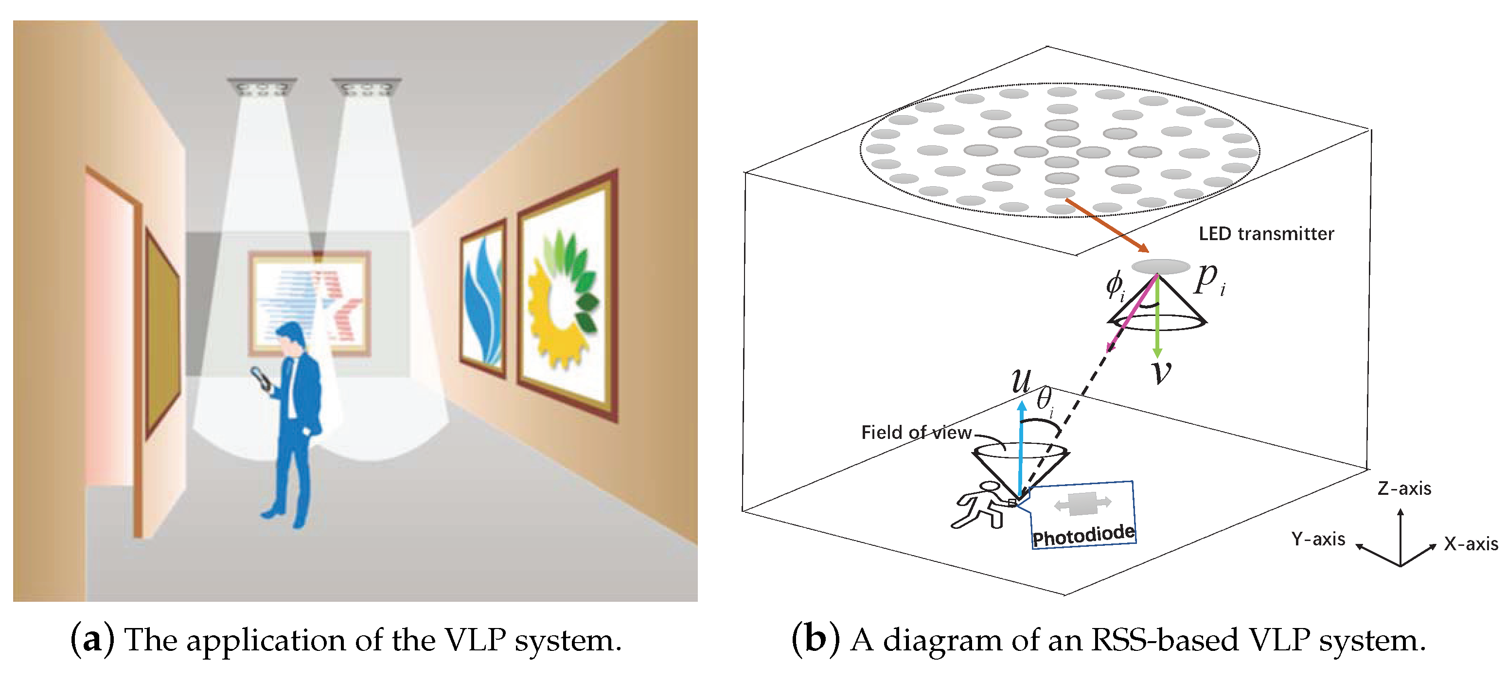
In a three-dimensional (3D) scenario, a VLP system composed of M LEDs is used to locate the user equipped with a photodiode (PD). We denote the position and orientation of the i-th LED as ${\mathbf{p}}_i\in {\mathbb{R}}^3$ and $\mathbf{v}\in {\mathbb{R}}^3$, which are known for $i=1,2,\dots ,M$. The position and orientation of the user need to be determined and are represented by ${\mathbf{x}}^o\in {\mathbb{R}}^3$ and ${\mathbf{u}}^o\in {\mathbb{R}}^3$, where the ${\ell }_2$ norm of vector ${\mathbf{u}}^o$ is one, i.e.,  $\parallel {\mathbf{u}}^o\parallel =1$. As illustrated in Figure 1, the LEDs are always installed in the upper part of the room, and the user should be in the range of light illumination.

The LEDs are able to communicate with the user using the Visible Light Communication (VLC) technique. Thus, the user can acquire the LED IDs of the VLC signals, and the received signal strength (RSS) corresponding to each LED, under the line-of-slight (LOS) link, is modeled as

$${\Phi }_i=\frac{{\Psi }_i}{2\pi }\frac{{(cos\left({\varphi }_i\right))}^{r_i}cos\left({\theta }_i\right)}{\parallel {\mathbf{x}}^o-{\mathbf{p}}_i{\parallel }^2},$$

(1)

where ${\Psi }_i=(r_i+1){\Gamma }_i{G}_i{P}_i{A}_i$, $A_i$ is the detection area of the PD and $r_i$ is Lambertian order of the i-th LED. For the Lambertian pattern of LED radiation, $r_i=-\frac{ln2}{lncos\left(A_{0.5}\right)}$, where $A_{0.5}$ is the semi-angle at the half power of the LEDs. Typically, $A_{0.5}=\frac{\pi }{3}$, and $r_i$ is equal to 1 [49]. ${\Gamma }_i$, $G_i$, and $P_i$ represent the gain of the optical filter, the gain of the optical concentrator, and the optical power of the i-th LED, respectively. Detailed definitions of ${\Gamma }_i$, $G_i$, and $P_i$ are given by [48,50], and they are generally available for a given LED and considered to be known. In addition, ${\varphi }_i$ and ${\theta }_i$ represent the irradiance angle and incidence angle of the i-th LED, respectively. ${\varphi }_i$ and ${\theta }_i$ should be within the field of view (FOV) angles ${\varphi }_F$ and ${\theta }_F$, i.e., $|{\varphi }_i| \le |{\varphi }_F|$ and $|{\theta }_i| \le |{\theta }_F|$. From the geometry relationship shown in Figure 1, the irradiance angle ${\varphi }_i$ and incidence angle ${\theta }_i$ are obtained by

$$\begin{array}{cc}\hfill & cos\left({\varphi }_i\right)=\frac{{({\mathbf{x}}^o-{\mathbf{p}}_i)}^T\mathbf{v}}{\parallel {\mathbf{x}}^o-{\mathbf{p}}_i\parallel },\hfill \end{array}$$

(2a)

$$\begin{array}{cc}\hfill & cos\left({\theta }_i\right)=\frac{{({\mathbf{p}}_i-{\mathbf{x}}^o)}^T{\mathbf{u}}^o}{\parallel {\mathbf{x}}^o-{\mathbf{p}}_i\parallel }.\hfill \end{array}$$

(2b)

Multiplying both sides by $\frac{-2\pi }{{\Psi }_i}$ and applying the definitions of (2a,b), we simplify (1) as

$$g_i^o=\frac{{({\mathbf{x}}^o-{\mathbf{p}}_i)}^T\mathbf{v}{({\mathbf{x}}^o-{\mathbf{p}}_i)}^T{\mathbf{u}}^o}{\parallel {\mathbf{x}}^o-{\mathbf{p}}_i{\parallel }^4},$$

(3)

where $g_i^o=\frac{-2\pi {\Phi }_i}{{\Psi }_i}$ and $r_i$ is considered to be one. The true $g_i^o$ is unavailable, and its measurable version is expressed as

$$g_i=g_i^o+\Delta g_i,$$

(4)

where $g_i$ is a measured value of $g_i^o$ and $\Delta g_i$ is additive noise, $i=1,2,\dots ,M$. Stacking all measurements yields a vector form $\mathbf{g}={[g_1,g_2,\dots ,g_M]}^T$. Similarly, collecting all the $\Delta g_i$ produces a vector $\Delta \mathbf{g}$, defined by $\Delta \mathbf{g}={[\Delta g_1,\Delta g_2,\dots ,\Delta g_M]}^T$. $\Delta g_i$ mainly includes shot noise and thermal noise. As a result, the vector form $\Delta \mathbf{g}$ obeys a zero-mean Gaussian distribution with covariance $\mathbf{\Sigma }=\mathrm{diag}\left({[{\sigma }_1^2,{\sigma }_2^2,\dots ,{\sigma }_M^2]}^T\right)$, where ${\sigma }_i^2$ is the variance of the total noise, $i=1,2,\dots ,M$.

Considering the user orientation as known or unknown, we aim at estimating the position ${\mathbf{x}}^o$ using the measured $\mathbf{g}$ in the VLP system, where the positions ${\mathbf{p}}_i$ and the orientation $\mathbf{v}$ are known. In addition, ${\mathbf{u}}^o$ should satisfy $\parallel {\mathbf{u}}^o\parallel =1$. Note that all LED orientations are assumed to be the same. This assumption is reasonable since all installed LEDs always have the same orientation as the luminaires. In addition, in the proposed problem, the Lambertian order $r_i$ considered as one. If $r_i$ is not equal to one and is near one, our proposed closed-form solution can be further refined using some numerical methods.

4. Closed-Form Solutions

In this section, we introduce the closed-form solutions in detail for the RSS-based VLP problem considering two cases: a known and unknown user orientation. For each case, the closed-form solution is divided into two stages. In  stage one, we establish the pseudo-linear equation in terms of unknown parameters using RSS measurements, and the user position is then estimated by applying the WLS method from the pseudo-linear equation. The stage-two solution refines the estimates obtained from the stage-one WLS solution. As a result, the performance of the stage-two solution becomes better than that of stage-one.

4.1. Known User Orientation

In this case, the user orientation is assumed to be known and directly equal to $\mathbf{u}$. Multiplying both sides of (3) by $\parallel {\mathbf{x}}^o-{\mathbf{p}}_i{\parallel }^4$ and expanding and rearranging the expression yield the following

$$\begin{array}{cc}\hfill & {\mathbf{a}}_i^T{\mathbf{x}}^o+4g_i{\left({\mathbf{p}}_i^T{\mathbf{x}}^o\right)}^2-{\mathbf{x}}^{oT}\mathbf{u}{\mathbf{v}}^T{\mathbf{x}}^o+2g_i{\mathbf{p}}_i^T{\mathbf{p}}_i{\mathbf{x}}^{oT}{\mathbf{x}}^o-4g_i{\mathbf{p}}_i^T\left({\mathbf{x}}^{oT}{\mathbf{x}}^o{\mathbf{x}}^o\right)+g_i{\left({\mathbf{x}}^{oT}{\mathbf{x}}^o\right)}^2\hfill \\ \hfill & +g_i{\mathbf{p}}_i^T{\mathbf{p}}_i{\mathbf{p}}_i^T{\mathbf{p}}_i-{\mathbf{p}}_i^T\mathbf{v}{\mathbf{p}}_i^T\mathbf{u}={\parallel {\mathbf{x}}^o-{\mathbf{p}}_i\parallel }^4\Delta g_i,\hfill \end{array}$$

(5)

where ${\mathbf{a}}_i={\mathbf{p}}_i^T\mathbf{u}\mathbf{v}+{\mathbf{p}}_i^T\mathbf{v}\mathbf{u}-4g_i{\mathbf{p}}_i^T{\mathbf{p}}_i{\mathbf{p}}_i$, $i=1,2,\dots ,M$. The terms $4g_i{\left({\mathbf{p}}_i^T{\mathbf{x}}^o\right)}^2$ and $2g_i{\mathbf{p}}_i^T{\mathbf{p}}_i{\mathbf{x}}^{oT}{\mathbf{x}}^o$ can be grouped in a more compact form. Applying the vector multiplying formula, we arrive at

$$\begin{array}{cc}\hfill & 4g_i{\left({\mathbf{p}}_i^T{\mathbf{x}}^o\right)}^2={\mathbf{b}}_{i,1}^T{\mathit{\rho }}^o,-{\mathbf{x}}^{oT}\mathbf{u}{\mathbf{v}}^T{\mathbf{x}}^o={\mathbf{b}}_{i,2}^T{\mathit{\rho }}^o,{\mathbf{p}}_i^T{\mathbf{p}}_i{\mathbf{x}}^{oT}{\mathbf{x}}^o={\mathbf{b}}_{i,3}^T{\mathit{\rho }}^o,\hfill \\ \hfill & {\mathit{\rho }}^o={[\mathrm{diag}{\left({\mathbf{x}}^o{\mathbf{x}}^{oT}\right)}^T,\mathrm{diag}{({\mathbf{x}}^o{\mathbf{x}}^{oT},1)}^T,\mathrm{diag}{({\mathbf{x}}^o{\mathbf{x}}^{oT},2)}^T]}^T,\hfill \\ \hfill & {\mathbf{b}}_{i,1}=4g_i{[\mathrm{diag}{\left({\mathbf{p}}_i{\mathbf{p}}_i^T\right)}^T,2\mathrm{diag}{({\mathbf{p}}_i{\mathbf{p}}_i^T,1)}^T,2\mathrm{diag}{({\mathbf{p}}_i{\mathbf{p}}_i^T,2)}^T]}^T,\hfill \\ \hfill & {\mathbf{b}}_{i,2}=-{[\mathrm{diag}{\left(\mathbf{v}{\mathbf{u}}^T\right)}^T,\mathrm{diag}{(\mathbf{v}{\mathbf{u}}^T,1)}^T+\mathrm{diag}{(\mathbf{v}{\mathbf{u}}^T,-1)}^T,\mathrm{diag}{(\mathbf{v}{\mathbf{u}}^T,2)}^T+\mathrm{diag}{(\mathbf{v}{\mathbf{u}}^T,-2)}^T]}^T,\hfill \\ \hfill & {\mathbf{b}}_{i,3}=2g_i{\mathbf{p}}_i^T{\mathbf{p}}_i[{\mathbf{1}}_3^T,{\mathbf{0}}_3^T{]}^T,\hfill \end{array}$$

(6)

where ${\mathit{\rho }}^o\in {\mathbb{R}}^6$. As a result, (5) is also rewritten as

$$\begin{array}{cc}\hfill & {\mathbf{a}}_i^T{\mathbf{x}}^o+{\mathbf{b}}_i^T{\mathit{\rho }}^o-4g_i{\mathbf{p}}_i^T\left({\mathbf{x}}^{oT}{\mathbf{x}}^o{\mathbf{x}}^o\right)+g_i{\left({\mathbf{x}}^{oT}{\mathbf{x}}^o\right)}^2\hfill \\ \hfill & +g_i{\mathbf{p}}_i^T{\mathbf{p}}_i{\mathbf{p}}_i^T{\mathbf{p}}_i-{\mathbf{p}}_i^T\mathbf{v}{\mathbf{p}}_i^T\mathbf{u}={\parallel {\mathbf{x}}^o-{\mathbf{p}}_i\parallel }^4\Delta g_i,\hfill \end{array}$$

(7)

where ${\mathbf{b}}_i={\mathbf{b}}_{i,1}+{\mathbf{b}}_{i,2}+{\mathbf{b}}_{i,3}$. Let the unknown vector be

$$\begin{array}{c}\hfill {\mathit{\phi }}^o={[\underset{3}{\underbrace{{\mathbf{x}}^{oT}}},\underset{6}{\underbrace{{\mathit{\rho }}^{oT}}},\underset{3}{\underbrace{{\mathbf{x}}^{oT}{\mathbf{x}}^o{\mathbf{x}}^{oT}}},\underset{1}{\underbrace{{\left({\mathbf{x}}^{oT}{\mathbf{x}}^o\right)}^2}}]}^T\in {\mathbb{R}}^{13}.\end{array}$$

(8)

For our proposed problem, the intended unknown is only ${\mathbf{x}}^o$, and the other introduced auxiliary variables are determined by the intended unknown. When the defined variables are considered to be independent of each other, (8) is considered to be a linear expression. As a result, the linear matrix form of (5) is given by

$$\begin{array}{c}\hfill {\mathbf{G}}_1{\mathit{\phi }}^o-{\mathbf{h}}_1={\mathit{\alpha }}_1,\end{array}$$

(9)

where ${\mathit{\alpha }}_1$ is the noise term and is given by ${\mathit{\alpha }}_1={\mathbf{B}}_1\Delta \mathbf{g}$, ${\mathbf{G}}_1$ is an $M\times 13$ matrix, and the i-th row of ${\mathbf{G}}_1$ is defined by

$$\begin{array}{c}\hfill {\left[{\mathbf{G}}_1\right]}_{i,:}=[{\mathbf{a}}_i^T,{\mathbf{b}}_i^T,-4g_i{\mathbf{p}}_i^T,g_i],\end{array}$$

(10)

where $i=1,2,\dots ,M$. In addition, the diagonal matrix ${\mathbf{B}}_1\in {\mathbb{R}}^{M\times M}$ and vector ${\mathbf{h}}_1\in {\mathbb{R}}^M$ are defined by

$$\begin{array}{cc}\hfill & {\left[{\mathbf{h}}_1\right]}_i=-g_i{\mathbf{p}}_i^T{\mathbf{p}}_i{\mathbf{p}}_i^T{\mathbf{p}}_i+{\mathbf{p}}_i^T\mathbf{v}{\mathbf{p}}_i^T\mathbf{u},\hfill \\ \hfill & {\left[{\mathbf{B}}_1\right]}_{i,i}=\parallel {\mathbf{x}}^o-{\mathbf{p}}_i{\parallel }^4\simeq {\parallel \mathbf{x}-{\mathbf{p}}_i\parallel }^4,\hfill \end{array}$$

(11)

where ${\mathbf{x}}^o$ is approximated by its estimated value $\mathbf{x}$. For the stage-one WLS solution, the estimate value $\mathit{\phi }$ of ${\mathit{\phi }}^o$ is given by

$$\begin{array}{c}\hfill \mathit{\phi }={\left({\mathbf{G}}_1^T{\mathbf{W}}_{{\mathit{\alpha }}_1}{\mathbf{G}}_1\right)}^{-1}{\mathbf{G}}_1^T{\mathbf{W}}_{{\mathit{\alpha }}_1}{\mathbf{h}}_1,\end{array}$$

(12)

where ${\mathbf{W}}_{{\mathit{\alpha }}_1}$ is called a weighting matrix and is approximately equal to the inverse of the covariance with respect to the noise term ${\mathit{\alpha }}_1$. As a result, ${\mathbf{W}}_{{\mathit{\alpha }}_1}$ is obtained by

$$\begin{array}{c}\hfill {\mathbf{W}}_{{\mathit{\alpha }}_1}={({\mathbf{B}}_1\mathbf{\Sigma }{\mathbf{B}}_1^T)}^{-1}.\end{array}$$

(13)

To efficiently solve problem (9), the matrix ${\mathbf{G}}_1$ needs to be full of rank. Thus, the number of measurements needs to be larger than that of the variables for the WLS solution (12). At least 13 non-collinear LEDs are required to uniquely locate the user when the user orientation is available and considered to be known.

Remark 1.

From (13), the solution of ${\mathbf{W}}_{{\mathit{\alpha }}_1}$ depends on ${\mathbf{B}}_1$, which is unavailable at the beginning due to the unknown position $\mathbf{x}$. It is known that the WLS solution is insensitive to the weighting matrix ${\mathbf{W}}_{{\mathit{\alpha }}_1}$. Initially, ${\mathbf{W}}_{{\mathit{\alpha }}_1}$ is set to an identity to yield a coarse estimate φ, which is used to form ${\mathbf{W}}_{{\mathit{\alpha }}_1}$. Thus, forming ${\mathbf{W}}_{{\mathit{\alpha }}_1}$ using a coarse estimate gives a better solution.

Extracting from the estimated $\mathit{\phi }$, we can obtain the stage-one WLS solution of ${\mathbf{x}}^o$ by $\mathbf{x}={\left[\mathit{\phi }\right]}_{1:3}$. When the RSS measurements are subject to noise, the estimate value $\mathit{\phi }$ also contains error. As a result, we have $\mathit{\phi }={\mathit{\phi }}^o+\Delta \mathit{\phi }$, where $\Delta \mathit{\phi }$ is the estimation error included in $\mathit{\phi }$. Since the noise term is ${\mathbf{B}}_1\Delta \mathbf{g}$ in the linear Equation (10), the estimation error $\Delta \mathit{\phi }$ is

$$\begin{array}{c}\hfill \Delta \mathit{\phi }={\left({\mathbf{G}}_1^T{\mathbf{W}}_{{\mathit{\alpha }}_1}{\mathbf{G}}_1\right)}^{-1}{\mathbf{G}}_1^T{\mathbf{W}}_{{\mathit{\alpha }}_1}{\mathbf{B}}_1\Delta \mathbf{g},\end{array}$$

(14)

where the noise in ${\mathbf{G}}_1$ is considered to be insignificant. Although ${\mathbf{G}}_1$ also contains noise due to the inaccurate $g_i$, it is negligible at low noise levels. As a result, the error $\Delta \mathit{\phi }$ is zero-mean, and its covariance, denoted by $\mathrm{cov}(\Delta \mathit{\phi })$, is given by

$$\begin{array}{c}\hfill \mathrm{cov}(\Delta \mathit{\phi })={\left({\mathbf{G}}_1^T{\mathbf{W}}_{{\mathit{\alpha }}_1}{\mathbf{G}}_1\right)}^{-1}.\end{array}$$

(15)

The variables defined in ${\mathit{\phi }}^o$ are coupled with each other, and the constrained relationships are not considered in the stage-one solution. Hence, the stage-one WLS solution performs poorly. In the following, we further refine the stage-one solution by exploiting the constrained relationships among the variables.

According to the definition of ${\mathit{\phi }}^o$, applying $\mathit{\phi }={\mathit{\phi }}^o+\Delta \mathit{\phi }$ directly produces

$$\begin{array}{c}\hfill {\mathbf{G}}_2{\mathbf{x}}^o-{\mathbf{h}}_2={\mathit{\alpha }}_2,\end{array}$$

(16)

where ${\mathit{\alpha }}_2={\mathbf{B}}_2\Delta \mathit{\phi }$. The detailed derivation and definition of (16) are provided in Appendix A. Accordingly, the accurate estimate in the stage-two WLS solution is

$$\begin{array}{c}\hfill \mathbf{x}={\left({\mathbf{G}}_2^T{\mathbf{W}}_{{\mathit{\alpha }}_2}{\mathbf{G}}_2\right)}^{-1}{\mathbf{G}}_2^T{\mathbf{W}}_{{\mathit{\alpha }}_2}{\mathbf{h}}_2,\end{array}$$

(17)

where ${\mathbf{W}}_{{\mathit{\alpha }}_2}$ is also a weighting matrix, obtained by

$$\begin{array}{c}\hfill {\mathbf{W}}_{{\mathit{\alpha }}_2}={\left({\mathbf{B}}_2\mathrm{cov}(\Delta \mathit{\phi }){\mathbf{B}}_2^T\right)}^{-1}.\end{array}$$

(18)

4.2. Unknown User Orientation

A small deviation in the user orientation will result in a large position estimation error. In this case, the user orientation ${\mathbf{u}}^o$ is assumed to be unknown and needs to be estimated together with the user position. For this case, the definition of unknown variables is slightly different from that of a known user orientation. However, the derivation procedure of the closed-form solution is similar. By considering the user orientation as unknown, (5) is also represented as

$$\begin{array}{cc}\hfill & -4g_i{\mathbf{p}}_i^T{\mathbf{p}}_i{\mathbf{p}}_i^T{\mathbf{x}}^o-{\mathbf{p}}_i^T\mathbf{v}{\mathbf{p}}_i^T{\mathbf{u}}^o+4g_i{\left({\mathbf{p}}_i^T{\mathbf{x}}^o\right)}^2+2g_i{\mathbf{p}}_i^T{\mathbf{p}}_i{\mathbf{x}}^{oT}{\mathbf{x}}^o+{\mathbf{p}}_i^T{\mathbf{u}}^o{\mathbf{x}}^{oT}\mathbf{v}+{\mathbf{p}}_i^T\mathbf{v}{\mathbf{x}}^{oT}{\mathbf{u}}^o\hfill \\ \hfill & -4g_i{\mathbf{p}}_i^T\left({\mathbf{x}}^{oT}{\mathbf{x}}^o{\mathbf{x}}^o\right)+g_i{\left({\mathbf{x}}^{oT}{\mathbf{x}}^o\right)}^2-{\mathbf{v}}^T{\mathbf{x}}^o{\mathbf{x}}^{oT}{\mathbf{u}}^o+g_i{\mathbf{p}}_i^T{\mathbf{p}}_i{\mathbf{p}}_i^T{\mathbf{p}}_i={\parallel {\mathbf{x}}^o-{\mathbf{p}}_i\parallel }^4\Delta g_i.\hfill \end{array}$$

(19)

Note that the term ${\mathbf{p}}_i^T{\mathbf{u}}^o{\mathbf{x}}^{oT}\mathbf{v}$ should be integrated with ${\mathbf{p}}_i^T\mathbf{v}{\mathbf{x}}^{oT}{\mathbf{u}}^o$ for the common variables. As a result, this yields

$$\begin{array}{c}\hfill {\mathbf{p}}_i^T{\mathbf{u}}^o{\mathbf{x}}^{oT}\mathbf{v}+{\mathbf{p}}_i^T\mathbf{v}{\mathbf{x}}^{oT}{\mathbf{u}}^o={\mathbf{p}}_i^T{\mathit{\tau }}^o,\end{array}$$

(20)

where ${\mathit{\tau }}^o={\mathbf{u}}^o{\mathbf{x}}^{oT}\mathbf{v}+{\mathbf{u}}^{oT}{\mathbf{x}}^o\mathbf{v}$. Thus, (19) is also rewritten as

$$\begin{array}{cc}\hfill & -4g_i{\mathbf{p}}_i^T{\mathbf{p}}_i{\mathbf{p}}_i^T{\mathbf{x}}^o-{\mathbf{p}}_i^T\mathbf{v}{\mathbf{p}}_i^T{\mathbf{u}}^o+({\mathbf{b}}_{i,1}^T+{\mathbf{b}}_{i,3}^T){\mathit{\rho }}^o+{\mathbf{p}}_i^T{\mathit{\tau }}^o-4g_i{\mathbf{p}}_i^T\left({\mathbf{x}}^{oT}{\mathbf{x}}^o{\mathbf{x}}^o\right)+g_i{\left({\mathbf{x}}^{oT}{\mathbf{x}}^o\right)}^2\hfill \\ \hfill & -{\mathbf{v}}^T{\mathbf{x}}^o{\mathbf{x}}^{oT}{\mathbf{u}}^o+g_i{\mathbf{p}}_i^T{\mathbf{p}}_i{\mathbf{p}}_i^T{\mathbf{p}}_i={\parallel {\mathbf{x}}^o-{\mathbf{p}}_i\parallel }^4\Delta g_i,i=1,2,\dots ,M.\hfill \end{array}$$

(21)

Let the unknown vector be

$$\begin{array}{cc}\hfill & {\mathit{\eta }}^o={[\underset{3}{\underbrace{{\mathbf{x}}^{oT}}},\underset{3}{\underbrace{{\mathbf{u}}^{oT}}},\underset{6}{\underbrace{{\mathit{\rho }}^{oT}}},\underset{3}{\underbrace{{\mathit{\tau }}^{oT}}},\underset{3}{\underbrace{{\mathbf{x}}^{oT}{\mathbf{x}}^o{\mathbf{x}}^{oT}}},\underset{1}{\underbrace{{\left({\mathbf{x}}^{oT}{\mathbf{x}}^o\right)}^2}},\underset{1}{\underbrace{{\mathbf{v}}^T{\mathbf{x}}^o{\mathbf{x}}^{oT}{\mathbf{u}}^o}}]}^T\in {\mathbb{R}}^{20}.\hfill \end{array}$$

(22)

Collecting all expressions in an ascending order of i produces a matrix form:

$$\begin{array}{c}\hfill {\mathbf{C}}_1{\mathit{\eta }}^o-{\mathbf{d}}_1={\mathit{\beta }}_1,\end{array}$$

(23)

where the noise term ${\mathit{\beta }}_1$ is given by ${\mathit{\beta }}_1={\mathit{\alpha }}_1$ and ${\mathbf{C}}_1$ and ${\mathbf{d}}_1$ are defined by

$$\begin{array}{cc}\hfill & {\left[{\mathbf{C}}_1\right]}_{i,:}={[-4g_i{\mathbf{p}}_i^T{\mathbf{p}}_i{\mathbf{p}}_i^T,-{\mathbf{p}}_i^T\mathbf{v}{\mathbf{p}}_i^T,{\mathbf{b}}_{i,1}^T+{\mathbf{b}}_{i,3}^T,{\mathbf{p}}_i^T,-4g_i{\mathbf{p}}_i^T,g_i,-1]}^T,\hfill \\ \hfill & {\left[{\mathbf{d}}_1\right]}_i=g_i{\mathbf{p}}_i^T{\mathbf{p}}_i{\mathbf{p}}_i^T{\mathbf{p}}_i,i=1,2,\dots ,M.\hfill \end{array}$$

(24)

According to (23), we obtain the stage-one WLS solution $\mathit{\eta }$ of ${\mathit{\eta }}^o$ by

$$\begin{array}{c}\hfill \mathit{\eta }={\left({\mathbf{C}}_1^T{\mathbf{W}}_{{\mathit{\beta }}_1}{\mathbf{C}}_1\right)}^{-1}{\mathbf{C}}_1^T{\mathbf{W}}_{{\mathit{\beta }}_1}{\mathbf{d}}_1.\end{array}$$

(25)

where ${\mathbf{W}}_{{\mathit{\beta }}_1}$ is equal to ${\mathbf{W}}_{{\mathit{\alpha }}_1}$ for ${\mathit{\beta }}_1={\mathit{\alpha }}_1$.

Remark 2.

Similar to ${\mathbf{W}}_{{\mathit{\alpha }}_1}$, ${\mathbf{W}}_{{\mathit{\beta }}_1}$ is set to an identity to produce a preliminary estimate of ${\mathbf{x}}^o$. Then, the preliminary estimate is used to form ${\mathbf{W}}_{{\mathit{\beta }}_1}$, which will yield an accurate solution for the unknowns.

According to the definition of ${\mathit{\eta }}^o$, the estimate values are obtained by

$$\begin{array}{c}\hfill \mathbf{x}={\left[\mathit{\eta }\right]}_{1:3},\mathbf{u}={\left[\mathit{\eta }\right]}_{4:6}.\end{array}$$

(26)

Similar to (14) and (15), the estimation error of $\mathit{\eta }$ is denoted as $\Delta \mathit{\eta }$, the covariance of which is given by

$$\begin{array}{c}\hfill \mathrm{cov}(\Delta \mathit{\eta })={\left({\mathbf{C}}_1^T{\mathbf{W}}_{{\mathit{\beta }}_1}{\mathbf{C}}_1\right)}^{-1}.\end{array}$$

(27)

For the case of an unknown user orientation, the orientation is estimated together with the position. In addition to the two intended parameters, the others included in ${\mathit{\eta }}^o$ are auxiliary variables and used to assist in establishing the linear expression. The constrained relationships among these variables should be further exploited in the stage-two WLS solution. Let us define the intended unknown vector as

$$\begin{array}{c}\hfill {\mathbf{y}}^o={[{\mathbf{x}}^{oT},{\mathbf{u}}^{oT}]}^T.\end{array}$$

(28)

The stage-two WLS solution is obtained by

$$\begin{array}{c}\hfill {\mathbf{C}}_2{\mathbf{y}}^o-{\mathbf{d}}_2={\mathit{\beta }}_2,\end{array}$$

(29)

where the error term ${\mathit{\beta }}_2$ is given by ${\mathit{\beta }}_2={\mathbf{D}}_2\Delta \mathit{\eta }$, the detailed derivation and the definition of (29) are given in Appendix B. In addition, the user orientation should satisfy $\parallel {\mathbf{u}}^o\parallel =1$. Hence, the following constraint it yielded

$$\begin{array}{c}\hfill {\mathbf{y}}^{oT}\mathbf{P}{\mathbf{y}}^o=1,\end{array}$$

(30)

where the matrix $\mathbf{P}$ is defined by

$$\begin{array}{c}\hfill {\left[\mathbf{P}\right]}_{4:6}={\mathbf{I}}_3.\end{array}$$

(31)

According to (29), the estimation problem can be represented as a constrained optimization problem

$$\begin{array}{cc}\hfill & \underset{{\mathbf{y}}^o}{min}{({\mathbf{C}}_2{\mathbf{y}}^o-{\mathbf{d}}_2)}^T{\mathbf{W}}_{{\mathit{\beta }}_2}({\mathbf{C}}_2{\mathbf{y}}^o-{\mathbf{d}}_2)\hfill \\ \hfill & \mathrm{s}.\mathrm{t}.{\mathbf{y}}^{oT}\mathbf{P}{\mathbf{y}}^o=1,\hfill \end{array}$$

(32)

where ${\mathbf{W}}_{{\mathit{\beta }}_2}={\left({\mathbf{D}}_2\mathrm{cov}(\Delta \mathit{\eta }){\mathbf{D}}_2^T\right)}^{-1}$. The optimal solution $\mathbf{y}$ should satisfy the Karush–Kuhn–Tucker (KKT) conditions,

$$\begin{array}{cc}\hfill & \mathbf{y}\left(\lambda \right)={({\mathbf{C}}_2^T{\mathbf{W}}_{{\mathit{\beta }}_2}{\mathbf{C}}_2+\lambda \mathbf{P})}^{-1}{\mathbf{C}}_2^T{\mathbf{W}}_{{\mathit{\beta }}_2}{\mathbf{d}}_2,\hfill \end{array}$$

(33a)

$$\begin{array}{cc}\hfill & \mathbf{y}{\left(\lambda \right)}^T\mathbf{P}\mathbf{y}\left(\lambda \right)=1.\hfill \end{array}$$

(33b)

$\lambda$ is Lagrange coefficient, and its optimal value is determined by solving the six-root equation

$$\begin{array}{c}\hfill \sum _{i=1}^3\frac{{\mu }_i}{{(1+{\gamma }_i\lambda )}^2}=1,\end{array}$$

(34)

where ${\mu }_i$ and ${\gamma }_i$ are defined in Appendix C. The desired $\lambda$ is found from the roots of Equation (34) and the following procedure is then carried out:

(a)

Solve the six roots of Equation (34) and discard the complex roots.

(b)

Put the obtained roots in (33a) and estimate the user position and orientation from $\mathbf{x}={\left[\mathbf{y}\right]}_{1:3}$ and $\mathbf{u}={\left[\mathbf{y}\right]}_{4:6}$.

(c)

Make the orientation sign consistent with that of the stage-one WLS solution as the final step.

The definition of matrix ${\mathbf{C}}_2$ and vector ${\mathbf{d}}_2$ requires the estimate obtained from the stage-one WLS solution of (25), in which the variables are considered to be independent of each other. To efficiently solve the WLS problem, the number of measurements needs to be greater than that of unknown variables. Accordingly, at least 20 non-collinear LEDs are required to uniquely determine the user position and orientation. The detailed closed-form solution for an unknown user orientation is illustrated in Algorithm 1.

Algorithm 1: Closed-form solution for an unknown user orientation

Input: ${\mathbf{p}}_i$, $\mathbf{v}$, $g_i$, Σ, $i=1,2,\dots ,M$

Output: $\mathbf{x}$, $\mathbf{u}$

(1). Stage-one WLS solution:

Create ${\mathbf{C}}_1$ and ${\mathbf{d}}_1$ using (24);

Estimate η by (25) considering ${\mathbf{W}}_{{\mathit{\beta }}_1}$ as the identity;

Extract the coarse estimate of the user position using (26);

Generate ${\mathbf{W}}_{{\mathit{\beta }}_1}$ equal to ${\mathbf{W}}_{{\mathit{\alpha }}_1}$ from (13);

Estimate η with generated ${\mathbf{W}}_{{\mathit{\beta }}_1}$ by (25) again;

Obtain the stage-one WLS solution by extracting from the new estimated η.

(2). Stage-two WLS solution:

Create ${\mathbf{C}}_2$, ${\mathbf{d}}_2$, and ${\mathbf{D}}_2$ using (A15) and (A16), where $\mathit{\eta }$ is an estimate of the stage-one WLS solution;

Generate ${\mathbf{W}}_{{\mathit{\beta }}_2}$ from the definition below (32);

Solve the optimal $\mathbf{y}$ with (33), where $\lambda$ is found from the six roots of Equation (34);

Obtain the final stage-two WLS solution by checking the orientation sign.

5. Performance Analysis

In this section, the CRBs of two cases are first derived. The CRB of a KUO is proven to be smaller than that of a UUO. In addition, we analyze the computational complexity of the proposed closed-form solutions.

5.1. CRB Derivation

In this subsection, the CRBs of the VLP estimation problem are first evaluated for two different cases: a KUO and a UUO. The CRB provides a lower bound for error variance based on the assumption of Gaussian noise, which is commonplace for VLP systems [20,32]. As a result, the CRB of the unknown parameters is equal to the inverse of the Fisher information matrix (FIM). When the user orientation is known, the only variable is the user position ${\mathbf{x}}^o$. For notation simplicity, we shall use the symbol ${\mathbf{\nabla }}_{\mathbf{a},\mathbf{b}}$ to denote the partial derivative, i.e.,

$${\mathbf{\nabla }}_{\mathbf{a}}\stackrel{\mathrm{def}}{=}\frac{\partial \mathbf{g}}{\partial {\mathbf{a}}^T}.$$

(35)

According to [51], the CRB of a known user orientation, denoted by ${\mathrm{CRB}}_{\mathrm{KUO}}\left({\mathbf{x}}^o\right)$, is given by

$$\begin{array}{c}\hfill {\mathrm{CRB}}_{\mathrm{KUO}}\left({\mathbf{x}}^o\right)={\left({\mathbf{\nabla }}_{{\mathbf{x}}^o}^T{\mathbf{\Sigma }}^{-1}{\mathbf{\nabla }}_{{\mathbf{x}}^o}\right)}^{-1}.\end{array}$$

(36)

${\mathbf{\nabla }}_{{\mathbf{x}}^o}$ is also defined by

$$\begin{array}{cc}\hfill & {\left[{\mathbf{\nabla }}_{{\mathbf{x}}^o}\right]}_{i,1:3}=\frac{{\mathbf{L}}_i{\mathbf{s}}_i}{\parallel {\mathbf{x}}^o-{\mathbf{p}}_i{\parallel }^3}\hfill \end{array}$$

(37a)

$$\begin{array}{cc}\hfill & {\mathbf{L}}_i=[{\mathbf{e}}_i,\mathbf{v},{\mathbf{u}}^o],\hfill \end{array}$$

(37b)

$$\begin{array}{cc}\hfill & {\mathbf{s}}_i={[-4{\mathbf{e}}_i^T\mathbf{v}{\mathbf{e}}_i^T{\mathbf{u}}^o,{\mathbf{e}}_i^T{\mathbf{u}}^o,{\mathbf{e}}_i^T\mathbf{v}]}^T,\hfill \end{array}$$

(37c)

where ${\mathbf{e}}_i$ is called the incident vector and is given by ${\mathbf{e}}_i=\frac{{\mathbf{x}}^o-{\mathbf{p}}_i}{\parallel {\mathbf{x}}^o-{\mathbf{p}}_i\parallel }$, $i=1,2,\dots ,M$. For the case of an unknown user orientation, the intended unknown parameters are ${\mathbf{y}}^o={[{\mathbf{x}}^{oT},{\mathbf{u}}^{oT}]}^T$, in which $\parallel {\mathbf{u}}^o\parallel =1$. In [48], the CRB of unknown user orientation is given; however, the FIM may be deficient-rank due to the constrained condition. In the following, we apply the constrained CRB formulation to derive the CRB. Let $\mathbf{F}$ be the FIM corresponding to the unconstrained estimation problem. When the user orientation is unknown, $\mathbf{F}$ is obtained by

$$\begin{array}{c}\hfill \mathbf{F}={[{\mathbf{\nabla }}_{{\mathbf{x}}^o},{\mathbf{\nabla }}_{{\mathbf{u}}^o}]}^T{\mathbf{\Sigma }}^{-1}[{\mathbf{\nabla }}_{{\mathbf{x}}^o},{\mathbf{\nabla }}_{{\mathbf{u}}^o}].\end{array}$$

(38)

where ${\mathbf{\nabla }}_{{\mathbf{x}}^o}$ is the same as that in (36), and ${\mathbf{\nabla }}_{{\mathbf{u}}^o}$ is defined by

$$\begin{array}{c}\hfill {\left[{\mathbf{\nabla }}_{{\mathbf{u}}^o}\right]}_{i,1:3}=\frac{{\mathbf{e}}_i^T\mathbf{v}{\mathbf{e}}_i^T}{\parallel {\mathbf{x}}^o-{\mathbf{p}}_i{\parallel }^2}.\end{array}$$

(39)

Expression (38) is also expressed as

$$\begin{array}{c}\hfill \mathbf{F}=\left[\begin{array}{cc}\mathbf{X}& \mathbf{Y}\\ {\mathbf{Y}}^T& \mathbf{Z}\end{array}\right],\end{array}$$

(40)

where

$$\begin{array}{cc}\hfill & \mathbf{X}={\mathbf{\nabla }}_{{\mathbf{x}}^o}^T{\mathbf{\Sigma }}^{-1}{\mathbf{\nabla }}_{{\mathbf{x}}^o},\hfill \end{array}$$

(41a)

$$\begin{array}{cc}\hfill & \mathbf{Y}={\mathbf{\nabla }}_{{\mathbf{x}}^o}^T{\mathbf{\Sigma }}^{-1}{\mathbf{\nabla }}_{{\mathbf{u}}^o},\hfill \end{array}$$

(41b)

$$\begin{array}{cc}\hfill & \mathbf{Z}={\mathbf{\nabla }}_{{\mathbf{u}}^o}^T{\mathbf{\Sigma }}^{-1}{\mathbf{\nabla }}_{{\mathbf{u}}^o}.\hfill \end{array}$$

(41c)

For the unconstrained estimation problem, the CRB of ${\mathbf{x}}^o$, denoted by ${\mathrm{CRB}}_{\mathrm{UUO}}\left({\mathbf{x}}^o\right)$, is the upper left $3\times 3$ matrix of ${\mathbf{F}}^{-1}$. Applying the partitioned matrix inversion formula produces

$$\begin{array}{c}\hfill {\mathrm{CRB}}_{\mathrm{UUO}}\left({\mathbf{x}}^o\right)={(\mathbf{X}-\mathbf{Y}{\mathbf{Z}}^{-1}{\mathbf{Y}}^T)}^{-1}.\end{array}$$

(42)

According to (41a–c), (42) is also rewritten as

$$\begin{array}{c}\hfill {\mathrm{CRB}}_{\mathrm{UUO}}\left({\mathbf{x}}^o\right)={\left({\mathbf{\nabla }}_{{\mathbf{x}}^o}^T\mathbf{K}{\mathbf{\nabla }}_{{\mathbf{x}}^o}\right)}^{-1},\end{array}$$

(43)

where $\mathbf{K}$ is defined as

$$\begin{array}{c}\hfill \mathbf{K}={\mathbf{\Sigma }}^{-1}-{\mathbf{\Sigma }}^{-1}{\mathbf{\nabla }}_{{\mathbf{u}}^o}{\left({\mathbf{\nabla }}_{{\mathbf{u}}^o}^T{\mathbf{\Sigma }}^{-1}{\mathbf{\nabla }}_{{\mathbf{u}}^o}\right)}^{-1}{\mathbf{\nabla }}_{{\mathbf{u}}^o}^T{\mathbf{\Sigma }}^{-1}.\end{array}$$

(44)

Comparing (43) with (36), we arrive at

$${\mathrm{CRB}}_{\mathrm{KUO}}\left({\mathbf{x}}^o\right)\le {\mathrm{CRB}}_{\mathrm{UUO}}\left({\mathbf{x}}^o\right).$$

(45)

According to (44), the presence of an unknown user orientation is equivalent to increasing the noise covariance by an extra term that is determined by ${\mathbf{\nabla }}_{{\mathbf{u}}^o}$ and the noise covariance $\mathbf{\Sigma }$.

Our proposed problem includes the constraint $\parallel {\mathbf{u}}^o\parallel =1$. According to [52], the constrained CRB formulation of unknown parameter ${\mathbf{y}}^o$, denoted by ${\mathrm{CCRB}}_{\mathrm{UUO}}\left({\mathbf{y}}^o\right)$, is expressed as

$${\mathrm{CCRB}}_{\mathrm{UUO}}\left({\mathbf{y}}^o\right)={\mathbf{F}}^{-1}-{\mathbf{F}}^{-1}\mathbf{q}{\left({\mathbf{q}}^T{\mathbf{F}}^{-1}\mathbf{q}\right)}^{-1}{\mathbf{q}}^T{\mathbf{F}}^{-1},$$

(46)

where the vector $\mathbf{q}$ is caused by the constraint and given by

$$\begin{array}{c}\hfill \mathbf{q}=\frac{\partial ({\left[{\mathbf{y}}^o\right]}_{4:6}^T{\left[{\mathbf{y}}^o\right]}_{4:6}-1)}{\partial {\mathbf{y}}^o}=2{\left[{\mathbf{y}}^o\right]}_{4:6}.\end{array}$$

(47)

Apparently, we have

$${\mathrm{CCRB}}_{\mathrm{UUO}}\left({\mathbf{x}}^o\right)\le {\mathrm{CRB}}_{\mathrm{UUO}}\left({\mathbf{x}}^o\right).$$

(48)

The constraint $\parallel {\mathbf{u}}^o\parallel =1$ indicates that there are two independent variables in the defined $\mathbf{u}$. As a result, ${\mathrm{CCRB}}_{\mathrm{UUO}}\left({\mathbf{x}}^o\right)$ is smaller than ${\mathrm{CRB}}_{\mathrm{UUO}}\left({\mathbf{x}}^o\right)$ due to fewer independent variables.

5.2. Computational Complexity

In this subsection, the complexity of the closed-form solutions is provided. When the WLS solution includes m equations and n unknown variables, its complexity is equal to $O(2m^{2}n+m{n}^2+mn+n^3+n^2)$ [53]. When the user orientation is known or unknown, the closed-form solutions are divided into two stages. For each case, the number of variables in the stage-two WLS solution is always irrelevant to M, and the complexity is mainly dominated by that of the stage-one WLS solution. Hence, we only compare the complexity of stage-one WLS solutions under the two different cases.

For the two different cases, the parameters of m and n are listed in

Table 1. Parameters in computing the complexity of closed-form solutions.

Solution	m	n
WLS for KUO in (12)	M	13
WLS for UUO in (25)	M	20

, where KUO and UUO represent known user orientation and unknown user orientation, respectively. Using the parameters listed in Table 1, we further calculate the complexity of these proposed closed-form solutions,

$$\begin{array}{cc}\hfill & \mathrm{Complexity}\mathrm{in}\left(12\right)\simeq O(26M^2+182M),\hfill \end{array}$$

(49a)

$$\begin{array}{cc}\hfill & \mathrm{Complexity}\mathrm{in}\left(25\right)\simeq O(40M^2+420M).\hfill \end{array}$$

(49b)

As a result, the complexity of a known user orientation is approximated by (49a). In contrast to the case of a known user orientation, the complexity of an unknown user orientation includes $\kappa$ WLS solutions for the choice of the optimal Lagrange coefficient $\lambda$. The complexity of an unknown user orientation is approximately equal to $O\left(\kappa (40M^2+420M)\right)$. Accordingly, the complexity of the UUO case is much greater than that of the KUO case. In contrast, we also derived the complexities of the trilateration-based method (denoted by “Trilateration”) [19], the NLS (denoted by “NLS”) [32], and the SLLS-SPAO [48], which are given by

$$\begin{array}{cc}\hfill & \mathrm{Complexity}\mathrm{of}\mathrm{Trilateration}\simeq O\left(13M^2\right),\hfill \end{array}$$

(50a)

$$\begin{array}{cc}\hfill & \mathrm{Complexity}\mathrm{of}\mathrm{NLS}\simeq O\left(M^2\log \frac{1}{ϵ}\right),\hfill \end{array}$$

(50b)

$$\begin{array}{cc}\hfill & \mathrm{Complexity}\mathrm{of}\mathrm{SLLS}\text{-}\mathrm{SPAO}\simeq O\left(40M^2\log \frac{1}{ϵ}\right),\hfill \end{array}$$

(50c)

where $ϵ$ is the solution accuracy of the NLS and the SLLS-SPAO.

6. Evaluation

The performance of the closed-form solutions was evaluated using simulations. Unless noted otherwise, the LEDs were deployed in a room of size 9 m × 9 m × 5 m. The LED positions in the x-axis and y-axis directions were randomly generated in the deployed region, and the height of the LEDs was restricted to the range of (4, 5) m. For our proposed VLP problem, all LED orientations need to be the same, and they are assumed to be downward, i.e., $\mathbf{v}={[0,0,-1]}^T$. The user position is set at ${\mathbf{x}}^o={[5,5,1]}^T$ m, and their orientation is considered to be upward, i.e., ${\mathbf{u}}^o={[0,0,1]}^T$. In addition, the other LED parameters are listed as follows, ${\Gamma }_i=2.25$, $G_i=1$, $A_i=1$ ${\mathrm{cm}}^2$, $P_i=2.2$ Watt, ${\varphi }_F={\theta }_F=\frac{\pi }{2}$, which implies that the user is within the range of all LED illuminations. The performance was evaluated using root mean square error (RMSE), defined by

$$\begin{array}{cc}\hfill & \mathrm{RMSE}\left(\mathbf{t}\right)=\sqrt{\frac{1}{GL}\sum _{g=1}^G\sum _{l=1}^L{\parallel {\mathbf{x}}_l^g-{\mathbf{x}}^o\parallel }^2},\hfill \end{array}$$

(51a)

$$\begin{array}{cc}\hfill & \mathrm{RMSE}\left(\mathbf{u}\right)=\sqrt{\frac{1}{GL}\sum _{g=1}^G\sum _{l=1}^L{\parallel {\mathbf{u}}_l^g-{\mathbf{u}}^o\parallel }^2},\hfill \end{array}$$

(51b)

where ${\mathbf{x}}_l^g$ and ${\mathbf{u}}_l^g$ are the estimates of user position and orientation in the l-th MC run for the g-th LED geometry configuration and $L=500$ and $G=20$ in our simulations. The signal-to-noise ratio (SNR) is given by $P_r^2{R}_p^2/{\sigma }_i^2$, where $R_p$ is the photoelectric conversion efficiency of a PD and $R_p=1$.

To the best of our knowledge, there are few solutions that do not require the initialization for the RSS-based VLP problem. For the KUO case, we will use the trilateration-based method (denoted by “Trilateration”) [19] as a baseline, and also compare the performance with that of the LS (denoted by “LS”) estimator [54] and the NLS (denoted by “NLS”) estimator [32], which employs the stage-one WLS solution as an initial guess. When the user orientation is unknown, the performance of the WLS solution is compared with that of the Gauss–Newton method (GNM) [21] and SLLS-SPAO [48], in which the stage-one WLS solution is regarded as the initial point. In addition, the CRB corresponding to two different cases is taken as a benchmark. The intention of the simulations is illustrated in

Table 2. Intention of simulations in eight scenarios.

Scenario	Varied Parameter	Examined Performance
1	SNR	CRB for KUO and UUO
2	SNR	RMSE of different solutions for the KUO case
3	SNR	RMSE of different solutions for the UUO case
4	number of LEDs	RMSE of different solutions for the KUO case
5	number of LEDs	RMSE of different solutions for the UUO case
6	room size	RMSE of different solutions for the KUO case
7	room size	RMSE of different solutions for the UUO case
8	user height	RMSE of different solutions for the KUO case

.

6.1. CRB Comparison under Two Cases

Scenario 1: The number of LEDs is set at 30, and their positions are generated randomly in the deployed room. For two different cases of a KUO and a UUO, the CRBs of user position and orientation estimation are plotted in Figure 2 as the noise increases. It is shown that the $\mathrm{CRB}\left({\mathbf{x}}^o\right)$ for a KUO is smaller than the $\mathrm{CCRB}\left({\mathbf{x}}^o\right)$ for a UUO, since the user orientation is also a variable in the UUO case. Hence, the solution of a KUO will perform better than that of a UUO. However, an accurate determination of the user orientation is not easy for VLP systems. Compared with the $\mathrm{CRB}\left({\mathbf{x}}^o\right)$ for a UUO, the $\mathrm{CCRB}\left({\mathbf{x}}^o\right)$ for a UUO is slighted reduced, confirming the result in (48). Hence, the constrained condition in (32) should be considered. As a result, the performance will also be slightly improved.

6.2. Performance Comparison with a Varying SNR

For the KUO and UUO cases, we also demonstrate the performance of the proposed solutions when the SNR varies.

Scenario 2: In this scenario, the performance of a KUO is examined with different solutions. M, the number of LEDs, is set to 30. Figure 3a shows the RMSE performance as the SNR is varied from −10 to 70. The trilateration-based method performs worst among these solutions, although it also does not require initialization. Based on the initial solution of stage-one WLS, the NLS method performs better due to its iterative refinements. However, the NLS performance still has a big gap regarding the CRB accuracy. Our proposed stage-two WLS solution performs well, especially at a large SNR. When the SNR is larger than 40, the performance of the stage-two WLS solution is close to the CRB accuracy.

In addition, the cumulative distributed function (CDF) of the positioning error was used to better assess the variability and reliability, and the results of these solutions are plotted in Figure 3b, where the SNR is kept at 30. It is shown that the 90% positioning error is less than 0.02 m for the stage-two WLS, 0.06 m for the NLS, 0.36 m for the stage-one WLS, 0.42 m for the LS, and 0.58 m for the trilateration method.

Scenario 3: The performance of a UUO is examined with our proposed solutions. Owing to more variables, the minimum number of LEDs needed for the UUO is increased compared with the KUO. Hence, the number of LEDs is set at 40 in this scenario. Figure 4a,b show the RMSE performance in the estimation of user position and orientation, respectively. Using the stage-one WLS solution as an initial guess, the GNM solution performs well. Unfortunately, its performance is still worse than that of the stage-two WLS solution. As is known, the SLLS-SPAO estimates the user position and orientation separately and does not consider the weighting matrix. Hence, the SLLS-SPAO provides a worse solution than our proposed stage-two WLS solution.

6.3. Performance with a Varying Number of LEDs

In this subsection, we also examine the performance of these solutions by varying M, the number of LEDs. Similarly, KUO and UUO cases are used to examine the performance.

Scenario 4: At an SNR from −10 to 20, our proposed solutions perform poorly. Hence, the SNR is set at 40 in this simulation. Figure 5 shows the RMSE performance in the estimation of the user position as M is varied from 15 to 60. As expected, the performance of these proposed solutions becomes better when the number of LEDs increases. Among the proposed solutions, the stage-two WLS solution performs best, and the performance comparison of these solutions is similar to the observations in Figure 3. When the number of LEDs is less than 30, the stage-one WLS solution has a big gap with the CRB accuracy. However, the performance becomes almost stable when the number of LEDs is larger than 30.

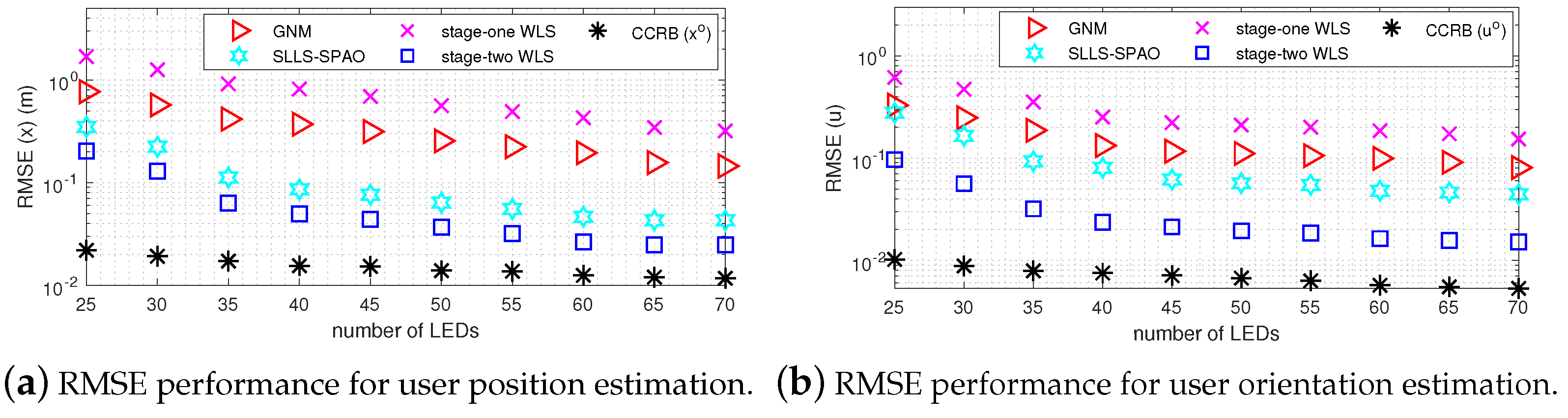
Scenario 5: Similar to the case of a KUO, the SNR is set to 40 for a UUO. Thus, the stage-one WLS solution can provide a reliable estimate and perform stably. The RMSE performance of user position and orientation estimation is shown in Figure 6a,b as the number of LEDs is increased from 25 to 70. As the number of LEDs increases, the performance of these solutions becomes better. The stage-one WLS provides a solution that does not require any initialization, although it performs poorly. The GNM and SLLS-SPAO perform well based on the initial solution of the stage-one WLS. However, they are still unable to provide a solution, the performance of which is sufficiently close to the CRB accuracy. In comparison, the performance of the stage-two WLS solution is closest to the CRB accuracy, which is consistent with the above observations.

6.4. Performance with a Varying Room Size

In the above simulations, the dimensions of the room were set at 9 m × 9 m. In this subsection, we examine the performance of these solutions with a varying room size. Similarly, we consider two different cases: a KUO and a UUO.

Scenario 6: The performance of the KUO case was investigated as the room size varies. The number of LEDs and the SNR are set at 30 and 40, respectively. Both the length and the width of room are varied from 10 m to 100 m, and the height of the LEDs is also randomly generated from (4, 5) m. The RMSE of the estimated user position is plotted in Figure 7. As shown in the figure, the RMSE performance degrades as the length of the room increases. The trilateration-based method performs worst among these solution due to its inaccurate ranging information, although it also does not require an initial guess for the solution. Compared with the stage-one WLS solution, our proposed stage-two WLS solution performs better by exploiting the constrained relationships among the variables.

Scenario 7: Similar to scenario 6, the room size was varied, and the performance of a UUO was examined. Both the number of LEDs and the SNR are set at 40. Figure 8 shows the RMSE of the user position as the length of the room was varied from 10 m to 100 m. As shown, the stage-two WLS solution still performs well even if the length of the room is increased to 100 m, and the RMSE of stage-two WLS solution is closest to the CRB accuracy among these solutions. The disadvantage of the GNM and SLLS-SPAO is that they require an initial guess. If the initial guess is not near the truth, the solutions may be trapped in local optima. In comparison, our proposed stage-one WLS can provide a solution that does not require initialization. In addition, the proposed stage-two WLS refines the estimates obtained from the stage-one WLS.

6.5. Performance with a Varying User Height

In the above simulations, the user height was kept at 1 m. As is known, the user height can be adjusted. In this subsection, we also examine the performance with a varying user height.

Scenario 8: We considered the KUO case, where the number of LEDs and the SNR are set at 30 and 40, respectively. The user position in the x-axis and y-axis direction is kept at (5, 5), and the user height is varied from 0.5 m to 5.0 m. Figure 9 illustrates the RMSE performance in the user position estimation as the user height increases. As shown in the figure, the RMSE is reduced with the increase in user height. When the user height is increased, the range between the user and LEDs becomes smaller. As a result, the measured RSS is accurate, and the performance improves. The height of the LEDs is also restricted to the range of (4, 5) m. Hence, the performance is stable when the user height is larger than 4.0 m. The gap between stage-two WLS solution and the CRB accuracy is the lowest among these solutions, indicating the advantage of stage-two WLS solution in the estimation of user position.

7. Conclusions and Future Works

Closed-form solutions are proposed to estimate the user position and orientation of IOT devices for the RSS-based VLP problem when the user orientation is assumed to be known or unknown. In the closed-form solutions, the user position and orientation are jointly estimated in two stages. The stage-two WLS solution refines the estimates obtained from the stage-one WLS. As a result, the performance becomes better by making use of the constrained relationships among the variables. When the SNR is larger than 40, the proposed closed-form solutions are able to accurately estimate the unknown parameters.

In the proposed problem, the user height is randomly generated from a specific range of rooms. In many situations, LEDs are always installed on the ceiling of a room, and the heights of all LEDs are the same. For this case, the unknown variables in the pseudo-linear form need to be redefined, and the dimensions of the variables can be further reduced. As a result, the required minimum number of LEDs is less than that of our VLP problem. In future work, the proposed closed-form solution will be further extended in new scenarios, such as LEDs with different orientations and users with known heights.

References

Ganti, D.; Zhang, W.; Kavehrad, M. VLC-based Indoor Positioning System with Tracking Capability Using Kalman and Particle Filters. In Proceedings of the 2014 IEEE International Conference on Consumer Electronics (ICCE), Las Vegas, NV, USA, 10–13 January 2014; pp. 476–477. [Google Scholar] [CrossRef]
Wu, X.; Mao, X.; Qi, H. Semidefinite Relaxation for Moving Target Localization in Asynchronous MIMO Systems. IEEE Trans. Commun.2023. [Google Scholar] [CrossRef]
Choi, J.; Kim, J.; Kim, N.S. Robust time-delay estimation for acoustic indoor localization in reverberant environments. IEEE Signal Process. Lett.2017, 24, 226–230. [Google Scholar] [CrossRef]
Jagadeesan, N.A.; Krishnamachari, B. Distributionally robust radio frequency localization. IEEE Trans. Signal Inf. Process. Netw.2019, 5, 390–403. [Google Scholar] [CrossRef]
Zhuang, Y.; Hua, L.; Wang, Q.; Cao, Y.; Gao, Z.; Qi, L.; Yang, J.; Thompson, J. Visible light positioning and navigation using noise measurement and mitigation. IEEE Trans. Veh. Technol.2019, 68, 11094–11106. [Google Scholar] [CrossRef]
Keskin, M.F.; Sezer, A.D.; Gezici, S. Optimal and robust power allocation for visible light positioning systems under illumination constraints. IEEE Trans. Commun.2019, 67, 527–542. [Google Scholar] [CrossRef]
Wang, Y.; Chen, M.; Yang, Z.; Luo, T.; Saad, W. Deep learning for optimal deployment of UAVs with visible light communications. IEEE Trans. Wirel. Commun.2020, 19, 7049–7063. [Google Scholar] [CrossRef]
Fang, X.; Li, X.; Xie, L. Angle-displacement rigidity theory with application to distributed network localization. IEEE Trans. Autom. Control2021, 66, 2574–2587. [Google Scholar] [CrossRef]
Menendez, J.M.; Steendam, H. Influence of the aperture-based receiver orientation on RSS-based VLP performance. In Proceedings of the International Conference on Indoor Positioning and Indoor Navigation (IPIN), Sapporo, Japan, 18–21 September 2017; pp. 1–7. [Google Scholar]
Kazikli, E.; Gezici, S. Hybrid TDOA/RSS based localization for visible lightsystems. Digit. Signal Process.2019, 86, 19–28. [Google Scholar] [CrossRef]
Bai, L.; Yang, Y.; Guo, C.; Xu, X.; Feng, C. Camera assisted received signal strength ratio algorithm for indoor visible light positioning. IEEE Commun. Lett.2019, 23, 2022–2025. [Google Scholar] [CrossRef]
Bakar, A.H.A.; Glass, T.; Tee, H.Y.; Alam, F.; Legg, M. Accurate visible light positioning using multiple photodiode receiver and machine learning. IEEE Trans. Instrum. Meas.2020, 70, 1–12. [Google Scholar] [CrossRef]
Li, Z.; Qiu, G.; Zhao, L.; Jiang, M. Dual-mode LED aided visible light positioning system under multi-path propagation: Design and demonstration. IEEE Trans. Wirel. Commun.2021, 20, 5986–6003. [Google Scholar] [CrossRef]
Zhang, W.; Chowdhury, M.I.S.; Kavehrad, M. Asynchronous indoor positioning system based on visible light communications. Opt. Eng.2014, 53, 1–9. [Google Scholar] [CrossRef]
Zhou, B.; Liu, A.; Lau, V. Joint user location and orientation estimation for visible light communication systems with unknown power emission. IEEE Trans. Wirel. Commun.2019, 18, 5181–5195. [Google Scholar] [CrossRef]
Shen, S.; Li, S.; Steendam, H. Simultaneous position and orientation estimation for visible lightsystems with multiple LEDs and multiple PDs. IEEE J. Sel. Areas Commun.2020, 38, 1866–1879. [Google Scholar] [CrossRef]
Liu, X.; Guo, L.; Yang, H.; Wei, X. Visible light positioning based on collaborative LEDs and edge computing. IEEE Trans. Comput. Soc. Syst.2022, 9, 324–335. [Google Scholar] [CrossRef]
Fang, X.; Xie, L.; Li, X. 3-D distributed localization with mixed local relative measurements. IEEE Trans. Signal Process.2020, 68, 5869–5881. [Google Scholar] [CrossRef]
Wu, X.; Qi, H. Motion parameter estimation for mobile sources using semidefinite programming. IEEE Trans. Mob. Comput.2023, 22, 1066–1080. [Google Scholar] [CrossRef]
Shawky, S.; El-Shimy, M.A.; El-Sahn, Z.A.; Rizk, M.R.M.; Aly, M.H. Improved VLC-based indoor positioning system using a regression approach with conventional RSS techniques. In Proceedings of the 13th International Wireless Communication and Mobile Computing, Valencia, Spain, 26–30 June 2017; pp. 904–909. [Google Scholar] [CrossRef]
Liu, X.; Wei, X.; Guo, L. DIMLOC: Enabling high-precision visible light localization under dimmable LEDs in smart buildings. IEEE Internet Things J.2019, 6, 3912–3924. [Google Scholar] [CrossRef]
Yang, H.; Zhong, W.D.; Chen, C.; Alphones, A.; Du, P. QoS-driven optimized design-based integrated visible light communication and positioning for indoor IoT networks. IEEE Internet Things J.2020, 7, 269–283. [Google Scholar] [CrossRef]
Li, Y.; Yang, P.; Renzo, M.D.; Xiao, Y.; Xiao, M.; Xiang, W. Precoded optical spatial modulation for indoor visible light communications. IEEE Trans. Commun.2021, 69, 2518–2531. [Google Scholar] [CrossRef]
Wu, X.; Li, Y.; Shen, Y.; Zhu, X. Efficient solutions for target localization in asynchronous MIMO networks. J. Netw. Comput. Appl.2022, 205, 103441. [Google Scholar] [CrossRef]
Wang, T.Q.; Sekercioglu, Y.A.; Neild, A.; Armstrong, J. Position accuracy of time-of-arrival based ranging using visible light with application in indoor localization systems. J. Light. Technol.2013, 31, 3302–3308. [Google Scholar] [CrossRef]
Noroozi, A.; Sebt, M.A.; Hosseini, S.M.; Amiri, R.; Nayebi, M.M. Closed-Form solution for elliptic localization in distributed MIMO radar systems with minimum number of sensors. IEEE Trans. Aerosp. Electron. Syst.2020, 56, 3123–3133. [Google Scholar] [CrossRef]
Sahin, A.; Eroglu, Y.S.; Güvenç, I.; Pala, N.; Yuksel, M. Accuracy of AOA-based and RSS-based 3D localization for visible light communications. In Proceedings of the 82nd IEEE Vehicular Technology Conference Fall 2015, Boston, MA, USA, 6–9 September 2015; pp. 1–5. [Google Scholar]
Majeed, K.; Hranilovic, S. Passive indoor visible light positioning system using deep learning. IEEE Internet Things J.2021, 8, 14810–14821. [Google Scholar] [CrossRef]
Herrnsdorf, J.; Dawson, M.D.; Strain, M.J. Positioning and data broadcasting using illumination pattern sequences displayed by LED arrays. IEEE Trans. Commun.2018, 66, 2582–5592. [Google Scholar] [CrossRef]
Bastiaens, S.; Goudos, S.K.; Joseph, W.; Plets, D. Metaheuristic optimization of LED locations for visible light positioning network planning. IEEE Trans. Broadcast.2021, 67, 894–908. [Google Scholar] [CrossRef]
Chen, F.; Huang, N.; Gong, C. RSS-based visible light positioning with unknown receiver tilting angle: Robust design and experimental demonstration. Opt. Express2022, 30, 39775–39793. [Google Scholar] [CrossRef]
Sharifi, H.; Kumar, A.; Alam, F.; Arif, K.M. Indoor localization of mobile robot with visible light communication. In Proceedings of the 2016 12th IEEE/ASME International Conference on Mechatronic and Embedded Systems and Applications (MESA), Auckland, New Zealand, 29–31 August 2016. [Google Scholar]
Le, T.; Ono, N. Closed-form and near closed-form solutions for TOA-based joint source and sensor localization. IEEE Trans. Signal Process.2016, 64, 4751–4766. [Google Scholar] [CrossRef]
Shao, H.; Zhang, X.; Wang, Z. Efficient closed-form algorithms for AOA based self-localization of sensor nodes using auxiliary variables. IEEE Trans. Signal Process.2014, 62, 2580–2594. [Google Scholar] [CrossRef]
Zhao, S.; Zhang, X.P.; Cui, X.; Lu, M. A closed-form localizationmethod utilizing pseudorange measurements from two nonsynchronized positioning systems. IEEE Internet Things J.2021, 8, 1082–1094. [Google Scholar] [CrossRef]
Wu, X.; Liu, Y.; Zhu, X.; Mo, L. Efficient solutions for MIMO radar localization under unknown transmitter positions and offsets. IEEE Trans. Wirel. Commun.2022, 21, 505–518. [Google Scholar] [CrossRef]
Wang, Y.; Ho, K.C. An asymptotically efficient estimator in closed-form for 3-D AOA localization using a sensor network. IEEE Trans. Wirel. Commun.2015, 14, 6524–6535. [Google Scholar] [CrossRef]
Wu, X.; Qi, H.; Xiong, N. Rank-one semidefinite programming solutions for mobile source localization in sensor networks. IEEE Trans. Netw. Sci. Eng.2021, 8, 638–650. [Google Scholar] [CrossRef]
Wang, W.; Wang, G.; Zhang, J.; Li, Y. Robust weighted least squares method for TOA-based localization under mixed LOS/NLOS conditions. IEEE Commun. Lett.2017, 21, 2226–2229. [Google Scholar] [CrossRef]
Amiri, R.; Behnia, F. An efficient weighted least squares estimator for elliptic localization in distributed MIMO radars. IEEE Signal Process. Lett.2017, 24, 902–906. [Google Scholar] [CrossRef]
Zhou, Z.; Kavehrad, M.; Deng, P. Indoor positioning algorithm using light-emitting diode visible light communications. Opt. Eng.2012, 51, 5009. [Google Scholar] [CrossRef]
Zhou, B.; Lau, V.; Chen, Q.; Cao, Y. Simultaneous positioning and orientating (SPAO) for visible light communications: Algorithm design and performance analysis. IEEE Trans. Veh. Technol.2018, 67, 11790–11804. [Google Scholar] [CrossRef]
Wu, C.; Yi, X.; Wang, W.; You, L.; Huang, Q.; Gao, X.; Liu, Q. Learning to Localize: A 3D CNN Approach to User Positioning in Massive MIMO-OFDM Systems. IEEE Trans. Wirel. Commun.2020, 20, 4556–4570. [Google Scholar] [CrossRef]
Bai, L.; Yang, Y.; Zhang, Z.; Feng, C.; Guo, C.; Cheng, J. A high-coverage camera assisted received signal strength ratio algorithm for indoor visible light positioning. IEEE Trans. Wirel. Commun.2021, 20, 5703–5743. [Google Scholar] [CrossRef]
Zhang, X.; Duan, J.; Fu, Y.; Shi, A. Theoretical accuracy analysis of indoor visible light communication positioning system based on received signal strength indicator. J. Light. Technol.2014, 32, 4180–4186. [Google Scholar] [CrossRef]
Stoica, P.; Ng, B.C. On the cramér-rao bound under parametric constraints. IEEE Signal Process. Lett.1998, 5, 177–179. [Google Scholar] [CrossRef]
Arora, S.; Barak, B. Computational Complexity: A Modern Approach; Cambridge University Press: Cambridge, UK, 2009. [Google Scholar]
Wang, K.; Liu, Y.; Hong, Z. RSS-based visible light positioning based on channel state information. Opt. Express2022, 30, 5683–5699. [Google Scholar] [CrossRef]
Figure 1.
VLP in an indoor environment.
Figure 2.
CRB comparison for user position and orientation estimations in scenario 1 as the SNR varies, .
Figure 3.
Performance comparison in scenario 2, . (a) RMSE comparison for user position estimation as SNR varies. (b) CDF of positioning error, SNR = 30.
Figure 4.
RMSE comparison in scenario 3 as SNR varies, .
Figure 5.
RMSE comparison for user position estimation in scenario 4 as M varies, SNR = 40.
Figure 6.
RMSE comparison in scenario 5 as M varies, SNR = 40.
Figure 7.
RMSE comparison for user position estimation in scenario 6 as room size varies, , SNR = 40.
Figure 8.
RMSE comparison for user position estimation in scenario 7 as room size varies, , SNR = 40.
Figure 9.
RMSE comparison for user position estimation in scenario 8 as user height varies, , SNR = 40.