Disturbance Frequency Trajectory Prediction in Power Systems Based on LightGBM Spearman

Abstract

Addressing the issue of reduced system inertia and significantly increased risk of system frequency deviation due to high penetration of renewable energy sources, this paper proposes a power system disturbance frequency trajectory prediction method based on light gradient boosting machine (LightGBM) Spearman to provide data support for advanced system stability judgment and the initiation of stability control measures. Firstly, the optimal cluster is determined by combining the K-means clustering algorithm with the elbow method to eliminate redundant electrical quantities. Subsequently, the Spearman coefficient is used to analyze feature correlation and filter out electrical quantities that are strongly correlated with frequency stability. Finally, a frequency trajectory prediction model is built based on LightGBM to achieve accurate prediction of disturbed frequency trajectories. The method is validated using a case study on the New England 10-machine 39-bus system constructed on the CloudPSS 4.0 full electromagnetic cloud simulation platform, and the results show that the proposed method has high accuracy in frequency trajectory prediction.

1. Introduction

Driving the transformation of the energy structure is a core task in building a new type of power system [1]. Under the incentive of multiple policies, the scale of new energy installations in China has climbed year by year [2]. By the end of 2022, China’s new energy installations, mainly wind and solar, reached 750 million kW, becoming the second main source of power after thermal power. It is expected that, by 2060, China’s new energy installation capacity could exceed 5 billion kW. With the surge in renewable energy installation capacity, the new type of power system faces more severe challenges in frequency stability [3].

The “Guidelines for Power System Security and Stability” national standard GB 38755-2019 [4] has added definitions and regulations regarding system frequency stability compared to its 2001 version, which stipulate the maintenance and recovery performance of system frequency after the power system endures major and minor disturbances [5]. It is evident that the criteria for frequency stability judgment and stability boundaries of the new type of power system have not changed substantially. However, the large-scale integration of a high proportion of renewable energy and the significant reduction in system inertia can lead to more severe frequency deviations when the system is disturbed [6,7]. Therefore, by proactively judging the trajectory of system frequency deviation to provide necessary data support [8] and implementing stability control measures early in destabilizing scenarios, the risk of system instability can be reduced, enhancing the dynamic stability of system frequency [9].

Traditional methods for predicting the dynamic frequency trajectory of a power system after disturbances are mostly based on physical models, including simplified frequency models and linearized modeling methods that incorporate wide-area measurement information. The former often utilize simplified models such as the average system frequency (ASF) [10] and system frequency response (SFR) [11], which equivalize the system to a single machine and focus on dynamic components that are closely related to system frequency, thereby reducing modeling complexity. Reference [12] combines wide-area measurement information and considers the DC power transmission equation to establish and solve the system state-space equation, achieving high accuracy and rate of prediction for dynamic frequency trajectories in AC/DC grids. To achieve frequency stability, reference [13] proposes a model predictive current and power (MPCP) control scheme and a model predictive voltage and power (MPVP) control method, predicting current, voltage, and power by modeling the state space of the system. However, with the continuous integration of new energy sources, these physical model-based prediction methods encounter difficulties in modeling and fail to balance computational speed and accuracy when dealing with large-scale new power systems [14]. With the development of artificial intelligence technology in recent years, machine learning methods have also been gradually applied to the task of predicting dynamic frequency trajectories after disturbances, such as the use of deep belief networks for post-disturbance frequency curve prediction in reference [15] and the prediction of AC/DC grid frequency curves based on SVM in reference [16]. For secondary frequency control, a back-propagation neural network (BPNN) is used in reference [17]. These methods have achieved good results in prediction accuracy and computation speed due to the excellent learning ability of machine learning technology for complex mappings between system inputs and outputs, but they still face difficulties in model training convergence, lack robustness, and have poor interpretability, with the effects on practical applications needing further validation. Unlike common machine learning methods, the LightGBM method in ensemble learning [18,19,20] adopts the gradient-boosting tree algorithm, integrating multiple decision trees to accomplish prediction tasks. It significantly improves prediction accuracy and generalization ability while greatly reducing training difficulty and exhibiting strong robustness, maintaining good predictive performance even with small datasets or large noise. Moreover, the feature importance assessment function of LightGBM enables researchers to analyze the impact of different input features on the prediction results, providing better interpretability of the method. Therefore, this paper implements fast and accurate prediction of the dynamic frequency trajectory of power systems after disturbances, based on the LightGBM method.

Feature engineering enhances data-driven model performance by constructing a more effective feature set through processes such as feature extraction, feature selection, and feature transformation. Power system data analysis involves a large amount of correlated data, and using all as input increases model computational complexity, causing feature redundancy and reducing model training efficiency and accuracy [21]. Feature selection algorithms are now widely used in power system analysis [22,23,24], with reference [25] building a critical feature subset of the power grid based on analyzing key power flow sections and feature combination effects. Reference [26], based on the SHAP method and explainable artificial intelligence theory, proposes a key feature selection method based on feature cumulative contribution rate and explainable artificial intelligence, improving the prediction accuracy of transient stability margin. Reference [27] combines normalized mutual information with the particle swarm optimization algorithm to select features strongly related to transient stability in stages. Compared to deep learning methods that require extensive pre-training, correlation coefficients that conform to statistical rules are simple to use, have a wide application range, and do not require pre-training, making them common tools for feature selection. References [28,29], based on the Spearman correlation coefficient, differentiates faults inside and outside new energy station areas, achieving longitudinal protection for outgoing lines. The issue of feature selection is rarely considered in existing dynamic frequency prediction problems. This paper uses the Spearman coefficient to filter sub-feature sets, reducing the model input dimension, while ensuring model generalizability and accuracy.

The main contributions of this paper are as follows:

(1)

A frequency trajectory prediction method for low-inertia systems’ frequency risk is proposed, which integrates the K-means clustering algorithm and the Spearman coefficient, obtaining electrical quantities that are strongly correlated with the system’s frequency stability;

(2)

Based on key electrical quantities, a frequency trajectory prediction model is built using LightGBM. This model achieves accurate prediction of disturbed frequency trajectories. The effectiveness of the proposed method is verified on the New England 10-machine 39-bus system, constructed on the CloudPSS full-electromagnetic cloud simulation platform.

2. Dynamic Frequency Trajectory Prediction Based on LightGBM

After a high proportion of new energy integration, the system exhibits a significant low-inertia characteristic. Following disturbances, the dynamic frequency of the system is more susceptible to substantial impacts. Obtaining dynamic frequency trajectories through predictive models in advance can provide the necessary data foundation and action time for system frequency stability assessment and the initiation of stability control measures. This has the potential to greatly optimize the operational capability of the system’s frequency stability.

The primary task of dynamic frequency trajectory prediction in power systems is to characterize the system’s evolutionary path based on operational data and disturbance information. This is achieved through methods such as time-domain simulations [30,31,32,33]. However, constrained by the mutual trade-off between prediction accuracy and computational efficiency, model-driven approaches are currently mostly applied in tasks within the power system domain, such as calculations and planning, where timeliness is less critical.

To address the timeliness requirements of online dynamic frequency trajectory prediction tasks in power systems, this paper proposes a data-driven LightGBM (Light Gradient Boosting Machine) frequency trajectory prediction model. This model represents an enhanced approach to Boosting ensemble learning, with its core idea involving the sequential construction of decision tree models. By aggregating the performance of multiple weak decision tree predictor models, it forms a predictive model with strong generalization performance and high prediction accuracy.

The LightGBM algorithm builds a new decision tree in each iteration, and the construction of each new tree is based on the completion of the preceding tree ensemble. The objective of each new tree is to correct the prediction errors of the previous tree ensemble. Therefore, the predicted values at each moment can be represented by

$$\begin{array}{c}{\widehat{y}}_i^{(0)}=0\hfill \\ {\widehat{y}}_i^{(1)}=f_1(x_i)={\widehat{y}}_i^{(0)}+f_1(x_i)\hfill \\ {\widehat{y}}_i^{(2)}=f_1(x_i)+f_2(x_i)={\widehat{y}}_i^{(1)}+f_2(x_i)\hfill \\ {\widehat{y}}_i^{(k)}=f_1(x_i)+\cdots +f_k(x_i)={\widehat{y}}_i^{(k-1)}+f_k(x_i)\hfill \end{array},$$

(1)

where ${\widehat{y}}_i^{(k)}$ represents the prediction for sample $x_i$ in the k-th round and $f_n(x_i)$ denotes the prediction for sample $x_i$ by the n-th decision tree.

The objective function of the decision tree constructed in the k-th round is

$$L^{(k)}=\sum _{i=1}^{n}l(y_i,{\widehat{y}}_i^{(k-1)}+f_k(x_i))+\mathsf{\Psi }(f_k),$$

(2)

where $L(k)$ represents the objective function for the k-th round, indicating the error between predicted values and actual values. A smaller value of $L(k)$ is preferable. $C(k)$ represents the complexity of the k-th decision tree, and it is directly proportional to the parameters in the decision tree model.

Substituting Equation (1) into Equation (2) yields

$$L^{(k)}=\sum _{i=1}^{n}l(y_i,{\widehat{y}}_i^{(k-1)}+f_k(x_i))+\sum _{j=1}^{k-1}\mathsf{\Psi }(f_j)+\mathsf{\Psi }(f_k),$$

(3)

where n represents the total number of samples to be predicted.

To minimize the objective function in the k-th round, analysis reveals that the second term in Equation (3) is a constant and can be ignored in the objective function, simplifying it to

$$L^{(k)}=\sum _{i=1}^{n}l(y_i,{\widehat{y}}_i^{(k-1)}+f_k(x_i))+\mathsf{\Psi }(f_k)$$

(4)

Expanding Equation (4) to the second order, using Taylor series and neglecting the constant term, we obtain

$$\begin{array}{c}{L}^{(k)}=\sum _{i=1}^n[l(y_i,{\widehat{y}}_i^{(k-1)})+\partial l(y_i,{\widehat{y}}_i^{(k-1)})f_k(x_i)\\ +\frac{1}{2}{\partial }^{2}l(y_i,{\widehat{y}}_i^{(k-1)})f_k^2(x_i)]+\mathsf{\Psi }(f_k)\\ =\sum _{i=1}^n[g_i{f}_k(x_i)+\frac{1}{2}{h}_i{f}_k^2(x_i)]+\mathsf{\Psi }(f_k)\end{array},$$

(5)

where $g_i$ and $h_i$ represent the first and second derivatives of the residual in the Taylor expansion, respectively. These are both known during the training of the tree generated in the k-th round.

The complexity of the model can be expressed as

$$\mathsf{\Psi }(f_k)=\gamma T+\frac{1}{2}\lambda \sum _{j=1}^T{w}_j^2,$$

(6)

where $W_j$ represents the values of the leaf nodes in decision tree j; T denotes the number of leaf nodes; and w and v represent the weights of the number of leaf nodes and the values of the nodes, respectively, in terms of model complexity.

By substituting the leaf nodes and weights of each decision tree into Equation (5), it can be expressed as

$$L^{(k)}=\sum _{j=1}^T[(\sum _{i\in I_j}{g}_i)w_j+\frac{1}{2}(\sum _{i\in I_j}{h}_i+\lambda )w_j^2]+\gamma T$$

(7)

Let Equation (7) contain

$$\begin{array}{c}{\displaystyle \sum _{i\in I_j}}{g}_i=G_j\hfill \\ {\displaystyle \sum _{i\in I_j}}(h_i+\lambda )=H_j\hfill \end{array}$$

(8)

Equation (7) can then be rewritten as

$$L^{(k)}=\sum _{j=1}^T[G_j{w}_j+\frac{1}{2}{H}_j{w}_j^2]+\gamma T$$

(9)

Equation (9) is a quadratic function with respect to $W_j$. It attains its minimum value if and only if

$$w_j=-\frac{G_j}{H_j+\lambda }$$

(10)

At this point, the objective function $L(k)$ attains its minimum value:

$$min{L}^{(k)}=-\frac{1}{2}\sum _{j=1}^T\frac{G_j^2}{H_j+\lambda }+\gamma T$$

(11)

Therefore, from Equations (10) and (11), it can be deduced that, to minimize the objective function of the current constructed decision tree, it should first obtain the bias, first derivative, and second derivative of the previous $k-1$ decision trees. By substituting these into Equations (10) and (11), the selection criteria for the current node’s decision tree value can be obtained.

While the aforementioned approach allows us to obtain rules for setting tree parameters and to minimize the objective function, when considering computational efficiency issues, it becomes challenging to traverse the combinatorial space of extremely large tree structures within a limited time. The LightGBM algorithm employs a histogram algorithm to accelerate the construction speed, effectively reducing the search space for tree structures and focusing on splitting comparisons for feature values that are deemed worthwhile to try.

Defining the system feature values and second-order gradient statistics as the basis for tree structure splitting in the k-th round can be formally represented as the set $D_k$. This can be expressed as

$$D_k=\{({x_1}_k,h_1),(x_{2k},h_2)\cdots (x_{nk},h_n)\}$$

(12)

A rank function can be defined for the set $D_k$:

$$r_k(z)=\frac{1}{{\sum }_{(x,h)\in D_k}h}\sum _{(x,h)\in D_k,x<z}h,$$

(13)

where $r_k(z)$ represents the proportion of numbers smaller than z, and it can serve as the basis for decision tree splitting selection.

Assuming the split point is $s_k^i$, according to Formula (13), the rule for selecting the split point is determined:

$$\begin{array}{c}|r_k(s_{k,j})-r_k(s_{k,j+1})|<\varphi \hfill \\ s.t.s_{k1}=\underset{i}{min}{x}_{ik}\hfill \end{array}$$

(14)

where $\varphi$ represents an approximate value of the interval width; $1/\varphi$ is used as an approximation coefficient for points within the interval range.

Combining the classification nodes from Equation (14) with the histogram algorithm, and by taking the difference between discrete plots of each node, LightGBM can obtain histograms of its sibling leaves with extremely low computational cost. This ensures a reduction in the search space for the tree structure while maintaining the predictive accuracy of the entire model. Therefore, in this study, LightGBM is adopted to construct a model for predicting the dynamic frequency trajectory of power system disturbances.

3. Feature Selection of Dynamic Frequency Prediction Based on Spearman Coefficient

After a major disturbance in the power system, the frequencies of various units in the system deviate from steady state, entering a dynamic fluctuation process. The system frequency during dynamic fluctuations is closely coupled with global system information. Therefore, it is necessary to comprehensively consider the combined impact of all generator units and busbars. However, the operating parameters of generators are diverse, and busbar information is complex and coupled. Using LightGBM to construct a dynamic frequency trajectory prediction model may lead to overfitting due to the high input dimensions. To address this, a feature selection method for dynamic frequency prediction in disturbed systems based on the Spearman coefficient is proposed. This method aims to ensure the training accuracy of the LightGBM model while reducing training time by selecting relevant features.

3.1. Feature Selection for Dynamic Frequency Prediction in the System

The overall system dynamic frequency is the rate of change of rotational speed caused by unbalanced power. It reflects the dynamic equilibrium state of energy exchange among various components such as generators, loads, and transmission lines in the power system. The center of inertia frequency of the system, denoted as ${\omega }_{\mathit{COI}}$, is defined as shown in Equation (15):

$${\omega }_{\mathit{COI}}=\sum _{i=1}^n(M_i{\omega }_i)/\sum _{i=1}^n{M}_i,$$

(15)

where $M_i$ represents the inertia time constant of the i-th generator, ${\omega }_i$ is the angular frequency of the i-th generator, and n is the number of generator units in the system.

The classical second-order generator model is

$$\left\{\begin{array}{c}\frac{d\delta }{dt}={\omega }_N\omega \hfill \\ \frac{d\omega }{dt}=\frac{1}{M}\left[P_M-P_E(\delta )-D\omega \right]\hfill \end{array}\right.,$$

(16)

where $\delta$ is the rotor angle of the generator, ${\omega }_N$ is the rated angular frequency of the generator, $\omega$ is the angular speed deviation, $PM$ and $PE$ are the mechanical and electromagnetic power of the generator, and D is the damping coefficient of the generator.

Substituting the system center of inertia frequency ${\omega }_{COI}$ into Equation (16), the dynamic frequency equation for a multi-machine system is

$$M_{\mathrm{sys}}\frac{d{\omega }_{\mathit{COI}}}{dt}=\sum _{i=1}^n{P}_{Mi}-\sum _{i=1}^n{P}_{Ei}-\sum _{i=1}^{n}D{\omega }_i$$

(17)

From the results, it is evident that the electromagnetic power and mechanical power of each generator are the main factors influencing ${\omega }_{COI}$. Further considering the relationship between the response of generator units and ${\omega }_{COI}$, additional input features are incorporated as

$$f_i=\frac{P_{Mi}\left(0^{+}\right)-P_{Ei}\left(0^{+}\right)}{M_i}-\frac{{\displaystyle \sum _{i=1}^n}{P}_{Mi}\left(0^{+}\right)-{\displaystyle \sum _{i=1}^n}{P}_{Ei}\left(0^{+}\right)}{M_{\mathrm{sys}}}$$

(18)

To complement the remaining features, a total of 20 input features are selected, as shown in

Table 1. Input features of dynamic frequency prediction.

Feature Number	Feature Description
f1	System load level
f2	Post-disturbance system power deficit value
f3	Degree of each generator’s response to dynamic frequency
f4	Root mean square of bus voltages after disturbance
f5–6	Mechanical power of generators before and after disturbance
f7–9	Total mechanical power of the system before and after disturbance
f9–10	Electromagnetic power of generators before and after disturbance
f11–12	Total electromagnetic power of the system before and after disturbance
f13–14	Reactive power of generators before and after disturbance
f15–16	Total reactive power of the system before and after disturbance
f17–18	Active and reactive loads of the system after disturbance
f19	Total active load of the system after disturbance
f20	Total reactive load of the system after disturbance

in this paper.

3.2. Feature Correlation Analysis for Disturbed System Dynamic Frequency Prediction

The Spearman’s rank correlation coefficient is a nonparametric measure of rank correlation that assesses the monotonic relationship between two variables. Compared to other correlation coefficients, the Kendall rank correlation coefficient is more suitable for measuring non-linear monotonic relationships and performs better when analyzing power system dynamic frequency features with strong nonlinearity.

The Spearman coefficient is an improvement on the Pearson correlation coefficient. Unlike the Pearson coefficient, which measures the strength of a linear relationship, the Spearman coefficient focuses on the monotonicity of the relationship between variables. The expression for the Spearman coefficient $r_s$ is

$$r_s=\frac{{\displaystyle \sum _{i=1}^n}\left(R_{X_i}-\overline{R_X}\right)\left(R_{Y_i}-\overline{R_Y}\right)}{\sqrt{{\displaystyle \sum _{i=1}^n}{\left(R_{X_i}-\overline{R_X}\right)}^2{\displaystyle \sum _{i=1}^n}{\left(R_{Y_i}-\overline{R_Y}\right)}^2}},$$

(19)

where $R_i$ denotes the rank of the i-th element of variable X, and $\overline{R}$ represents the mean rank of all elements.

The range of the Spearman coefficient is from −1 to 1, where 1 indicates a perfect positive correlation between variables, −1 indicates a perfect negative correlation, and 0 signifies no correlation between the variables.

Unlike other correlation coefficients, the Spearman correlation coefficient calculates correlations based on ranks rather than the actual values, making it less sensitive to outliers. In rank-based calculations, the actual numerical magnitude of data values is transformed into their ranking order. Since the ranking order is not influenced by outliers, the Spearman coefficient offers better robustness compared to the Pearson correlation coefficient. The comparison of features between Spearman and other common correlation coefficients is shown in

Table 2. Comparison of common correlation coefficient properties.

Category	Applicable Conditions	Rank Sensitivity	Sensitivity to Outliers
Spearman	Approximately Monotonic	Yes	No
Pearson	Linear Relationship	No	Yes
Kendall	Non-Linear Relationship	Yes	No

.

From the above table, it can be seen that the Pearson coefficient is sensitive to outliers and that the Kendall coefficient requires inputs as non-linear rank variables, which contradicts the requirements of dynamic frequency prediction tasks. The Spearman coefficient is sensitive to ordering, insensitive to outliers, and suitable for time series of dynamic frequency features, thereby enhancing the model’s resistance to interference.

3.3. Trajectory Prediction Based on the LightGBM Spearman Method

The Process for Predicting the Frequency Trajectory of a Disturbed Electric Power System and the Model Evaluation Metrics Are as Follows The process for predicting the frequency trajectory of a disturbed electric power system constructed in this paper is shown in Figure 1.

Figure 1 outlines a four-step process for predicting the frequency trajectory of a disturbed electric power system:

(1)

Simulation Model Construction: Utilize the CloudPSS full electromagnetic cloud simulation platform to build an IEEE 39-node electromagnetic simulation model. Set typical active power disturbances in the system and record the transient process data of electrical quantities at system nodes to form a frequency prediction dataset;

(2)

Clustering and Feature Selection: Apply the K-means algorithm to cluster related electrical quantities for frequency prediction. Determine the optimal number of clusters using the elbow method. Based on the clustering results, identify and eliminate similar redundant feature quantities;

(3)

Feature Correlation and Dimension Reduction: Calculate the correlation between the redundant-free feature quantities and the post-disturbance frequency trajectory of the system. Select feature quantities sensitive to the frequency trajectory to further reduce the dimensions of the model’s input;

(4)

Model Construction and Evaluation: Build a LightGBM model for predicting frequency trajectory. Use the dimension-reduced feature quantities obtained in step (3) as inputs to train the prediction model. Assess the model’s performance using various evaluation metrics.

To validate the performance of the frequency trajectory prediction proposed in this paper, Mean Absolute Error (MAE), Mean Square Error (MSE), and R Squared (R²) are used as evaluation metrics. The error functions are

$$MAE\left(X,h\right)=\frac{1}{m}{\sum }_{i=1}^m\left|h\left(x_i\right)-y_i\right|,$$

(20)

$$MSE\left(X,h\right)=\frac{1}{m}{\sum }_{i=1}^m{\left(h\left(x_i\right)-y_i\right)}^2,$$

(21)

$$R^2=1-\frac{{\sum }_{i=1}^m{\left(h\left(x_i\right)-y_i\right)}^2/m}{{\sum }_{i=1}^m{\left(\overline{y}-y_i\right)}^2/m}=1-\frac{MSE\left(X,h\right)}{Var\left(y\right)}$$

(22)

4. Case Study Analysis

4.1. Validation Case Study Introduction

This article validates the proposed method using the New England 10-machine 39-bus system test case. The simulation software employed is the CloudPSS 4.0 digital twin cloud platform. Three hundred different rated load levels are set between 50% and 100%. For each load level, one generator is taken offline in a rotating manner to simulate system faults. Data samples of the system are obtained through electromagnetic transient simulations, with a simulation duration of 8 s. The generator outage occurs in the 4th second and is cleared 100 milliseconds later. The input features for each sample are presented in Table 1. Over 3000 simulation data sets are collected and divided into a training set and a testing set with a 5:1 ratio. This dataset construction is for building a predictive model of dynamic frequency trajectories for the disturbed system.

4.2. Feature Selection Result Analysis

To improve the model prediction efficiency and avoid interference from irrelevant features, feature selection is performed on the features in

Table 3. Normalized weights for disturbance trajectory prediction features.

Feature	Feature Quantity	Weight
f2	Post-Disturbance System Power Deficit	0.1499
f1	System Load Level	0.1057
f4	Root Mean Square of Bus Voltages after Disturbance	0.0876
f16	Total Reactive Power of the System after Disturbance	0.0789
f11	Total Electromagnetic Power of the System Before and after Disturbance	0.0783
f9	Electromagnetic Power of Generators Before Disturbance	0.0781
f10	Electromagnetic Power of Generators after Disturbance	0.0724
f14	Reactive Power of Generators after Disturbance	0.0684
f12	Total Electromagnetic Power of the System after Disturbance	0.0634
f17	Active Load of the System after Disturbance	0.0582
f3	Degree of Each Generator’s Response to Dynamic Frequency	0.0391
f20	Total Reactive Load of the System after Disturbance	0.0361
Total	Twelve Features	0.9161

using the Spearman correlation analysis method. The importance of each feature, as calculated, is normalized and then sorted, as shown in Figure 2.

From the graph, it can be observed that there are significant differences in the weights of different features. It is necessary to perform feature selection to improve model prediction efficiency. Considering both feature importance and computational efficiency, the normalized weights are arranged from largest to smallest, and features are selected such that their cumulative sum reaches 90% as the final input. The normalized weights and weighted sum of features for disturbed trajectory prediction are shown in Table 3.

From the table, it can be seen that 12 features were ultimately selected as model inputs, and the sum of the weights of these features was 91.61%, covering most of the relevant information. The table also reveals that the most heavily weighted feature is the power deficit value of the disturbed system, followed by the system load level. This aligns with intuition, as the power deficit of the system has the highest correlation with frequency, resulting in its largest weight. By removing less-correlated features, a balance is struck between training efficiency and prediction accuracy of the model.

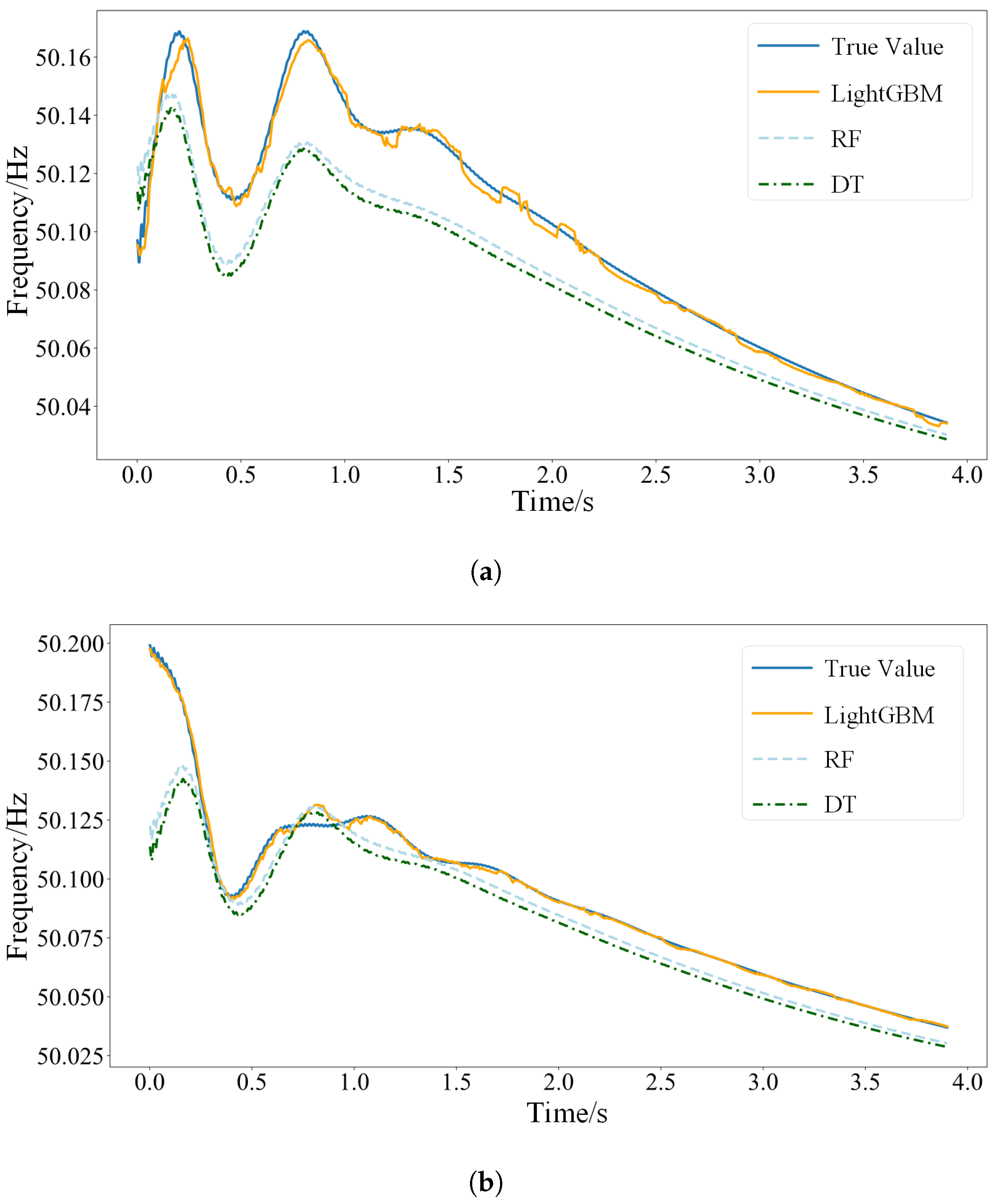
4.3. Frequency Prediction Result Analysis

The features selected in former section are individually fed into Long Short-Term Memory Network (LSTM), Convolutional Neural Network (CNN), Back-Propagation Neural Network (BPNN), decision tree (DT), random forest (RF), and LightGBM models for comparison. The comparison of the all algorithms with LightGBM is illustrated in

Table 4. Performance of multi-model trajectory prediction on the test dataset.

Index	LightGBM–Spearman			LSTM	CNN	BPNN	DT	RF
Number of features	12	10	8	12	12	12	12	12
MSE/10−4 Hz	1.131	1.610	1.842	1.597	1.602	1.687	34.256	21.214
MAE/10−2 Hz	2.567	2.997	3.025	2.732	2.796	2.844	14.096	10.013
R2	0.989	0.984	0.981	0.981	0.979	0.973	0.605	0.771

, while the comparison of the latter two algorithms with LightGBM is depicted in Figure 3. All deep learning models employ the same optimizer, configured with identical learning rates and training epochs. Non-deep learning models are trained until convergence. All algorithms utilize the same training and testing datasets, and their performance is quantified using identical evaluation metrics, ensuring the fairness of the experiments.

From Figure 3, it can be observed that, in both fault scenarios, LightGBM can closely follow the real frequency values and can exhibit higher prediction accuracy compared to RF and DT methods. Table 4 further demonstrates that LightGBM outperforms the other three models in terms of performance metrics, with the lowest MSE and MAE and the highest R² score when the number of features is the same. Its MSE is only 0.133 × 10⁻⁴ Hz, significantly smaller than RF and DT methods, and is smaller than the other methods, indicating the highest precision. Compared to deep learning models including LSTM, CNN, and BPNN, LightGBM–Spearman presents better performance as well. The R² score of 0.984 is higher than the other four methods, and, when features are reduced, the LightGBM–Spearman still shows high accuracy, confirming the effectiveness of this approach in predicting actual values.

4.4. Analysis of Prediction Results with Different Feature Combinations

To further demonstrate the necessity and effectiveness of feature selection, different subsets of features were used, including those with weight sums of 50%, 70%, 90%, and 100%, and randomly selecting 12 features, which were then fed into the LightGBM model for prediction. The various metrics and the duration of model training are presented in

Table 5. Influence of feature weight combinations on trajectory prediction.

Feature Weight Sum	MSE/10−5 Hz	MAE/10−3 Hz	R2	Training Time (s)
50%	2.303	3.579	0.973	7.06
70%	1.612	2.992	0.981	8.03
90%	1.335	2.723	0.984	8.76
Random 12 Features	5.643	7.016	0.915	8.93
All Features	1.432	2.853	0.983	9.48

.

From the table, it can be observed that, when fewer features are selected, the model training time is shorter, but the final accuracy also decreases. On the other hand, when all features are selected, although the model has access to more information, it also includes a significant amount of low-correlation data that are not conducive to model analysis and prediction, resulting in decreased accuracy. Additionally, randomly selecting 12 features leads to a significant drop in model accuracy. Therefore, it is necessary to use the Spearman correlation coefficient method to select highly correlated features as model inputs. In practical engineering applications, feature selection should strike a balance between model training efficiency and prediction accuracy based on specific circumstances.

5. Conclusions

This paper presents a dynamic frequency prediction method based on the Spearman correlation coefficient and LightGBM. Utilizing the Spearman correlation coefficient for feature selection reduces the complexity of model prediction, enhancing efficiency and accuracy. LightGBM is employed for frequency prediction using the selected features. Simulation results indicate that LightGBM reduces the MSE and MAE by up to 96.1% and 80.7% compared to other algorithms. When predicting with different feature combinations using LightGBM, the results show that features selected through the Spearman correlation coefficient method effectively balance model training efficiency and prediction accuracy. With only 70% of the features used in prediction tasks, the MSE is reduced by 6.77%, and the timeliness is improved by 7.59%. In practical engineering applications, different feature sets with varying weights can be chosen according to specific requirements.

References

1. Kang, C.Q.; Du, E.S.; Guo, H.Y.; Li, Y.W.; Fang, Y.C.; Zhang, N.; Zhong, H.W. Primary Exploration of Six Essential Factors in New Power System. Power Syst. Technol. 2023, 42, 1741–1750. [Google Scholar]
2. Lai, Q.P.; Xiao, T.N.; Li, D.S.; Shen, C. Low Voltage Ride-through Modeling for Wind Turbines Based on Neural ODEs. J. Syst. Simul. 2022, 34, 2546–2556. [Google Scholar]
3. Wang, M.J.; Guo, J.B.; Ma, S.C. Review of Transient Frequency Stability Analysis and Frequency Regulation Control Methods for Renewable Power Systems. Proc. CSEE 2023, 43, 1672–1694. [Google Scholar]
4. GB 38755-2019; Guidelines for Safety and Stability of Power Systems. State Administration for Market Regulation: Beijing, China, 2019.
5. Sun, H.; Xu, S.; Xu, T.; Bi, J.; Zhao, B.; Guo, Q.; He, J.; Song, R. Research on Definition and Classification of Power System Security and Stability. Proc. CSEE 2022, 42, 7796–7808. [Google Scholar]
6. Dong, W.J.; Liu, K.Y.; Wang, Y.L.; Li, X.Z.; Hao, Y. Adaptive Control Method of High Proportion Distributed Generation Connected to Distribution Network. J. Syst. Simul. 2020, 32, 2052–2058. [Google Scholar]
7. Lu, Z.X.; Jiang, J.H.; Qiao, Y.; Min, Y.; Li, H. A Review on Generalized Inertia Analysis and Optimization of New Power Systems. Proc. CSEE 2023, 43, 1754–1776. [Google Scholar]
8. Wang, Q.; Li, F.; Tang, Y.; Xu, Y. Integrating Model-Driven and Data-Driven Methods for Power System Frequency Stability Assessment and Control. IEEE Trans. Power Syst. 2019, 34, 4557–4568. [Google Scholar] [CrossRef]
9. Zhao, Q.Q.; Wang, X.R. A fast predictive algorithm for power system post disturbances steady frequency. Power Syst. Prot. Control 2011, 39, 72–77. [Google Scholar]
10. Chan, M.L.; Dunlop, R.D.; Schweppe, F. Dynamic Equivalents for Average System Frequency Behavior Following Major Disturbances. IEEE Trans. Power Appar. Syst. 1972, PAS-91, 1637–1642. [Google Scholar] [CrossRef]
11. Anderson, P.M.; Mirheydar, M. A low-order system frequency response model. IEEE Trans. Power Syst. 1990, 5, 720–729. [Google Scholar] [CrossRef]
12. Peng, A.; Teng, Y.; Wang, X. Prediction Algorithm of Steady Frequency after Disturbances Considering Emergency DC Power Support. Autom. Electr. Power Syst. 2017, 41, 92–99. [Google Scholar]
13. Shan, Y.; Hu, J.; Chan, K.W.; Fu, Q.; Guerrero, J.M. Model Predictive Control of Bidirectional DC–DC Converters and AC/DC Interlinking Converters—A New Control Method for PV-Wind-Battery Microgrids. IEEE Trans. Sustain. Energy 2019, 10, 1823–1833. [Google Scholar] [CrossRef]
14. Yang, H.; Meng, Q.; Zhang, Y.; Hao, Z.; He, J. An Online Prediction Model of Power System Frequency Nadir Based on Polynomial Fitting of Power-frequency Characteristics. Proc. CSEE 2022, 42, 115–125. [Google Scholar]
15. Zhang, Y.; Wen, D.; Wang, X.; Lin, J. A Method of Frequency Curve Prediction Based on Deep Belief Network of Post-disturbance Power System. Proc. CSEE 2019, 39, 5095–5104. [Google Scholar]
16. Hu, Y.; Wang, X.; Teng, Y. Frequency Stability Control Method of AC/DC Power System Based on Multi-layer Support Vector Machine. Proc. CSEE 2019, 39, 4104–4118. [Google Scholar]
17. Shan, Y.; Hu, J.; Shen, B. Distributed Secondary Frequency Control for AC Microgrids Using Load Power Forecasting Based on Artificial Neural Network. IEEE Trans. Ind. Inform. 2024, 20, 1651–1662. [Google Scholar] [CrossRef]
18. Yu, L.; Wang, Z.; Hao, Y.; Yan, X.; Zhang, L.; Yan, G.; Wen, Y. XGBoost-based Power System Dynamic Frequency-Response Curve Prediction. Electr. Power Constr. 2023, 44, 74–81. [Google Scholar]
19. Zhang, L.; Li, H.; Xiong, Z.; Guo, Z.; Ye, J.; Li, Z.; Yang, N.; Cai, Y. Short-Term Prediction Method Based on Interpretable XGBoost for Power System Inertia. Electr. Power Constr. 2023, 44, 22–30. [Google Scholar]
20. Bao, H.; Wu, Y.; Zhang, G.; Li, J.; Guo, X.; Li, J. Net Load Forecasting Method Based on Feature-Weighted Stacking Ensemble Learning. Electr. Power Constr. 2022, 43, 104–116. [Google Scholar]
21. Wang, Y.; Tai, K.; Song, Y.; Kou, R.; Zheng, Z.; Zeng, Q. Research on Double-Deck Traceability Identification Method of Commutation Failure in HVDC System. IEEE Access 2021, 9, 108392–108401. [Google Scholar] [CrossRef]
22. Zheng, Z.; Xu, Y.; Mili, L.; Liu, Z.; Korkali, M.; Wang, Y. Obuservability analysis of a power system stochastic dynamic model using a derivative-free approach. IEEE Trans. Power Syst. 2021, 36, 5834–5845. [Google Scholar] [CrossRef]
23. Xu, Y.; Wang, Q.; Mili, L.; Zheng, Z.; Gu, W.; Lu, S.; Wu, Z. A data-driven koopman approach for power system nonlinear dynamic observability analysis. IEEE Trans. Power Syst. 2023. [Google Scholar] [CrossRef]
24. Xu, Y.; Mili, L.; Sandu, A.; von Spakovsky, M.R.; Zhao, J. Propagating uncertainty in power system dynamic simulations using polynomial chaos. IEEE Trans. Power Syst. 2018, 34, 338–348. [Google Scholar] [CrossRef]
25. Mehmood, F.; Ghani, M.U.; Ghafoor, H.; Shahzadi, R.; Asim, M.N.; Mahmood, W. EGD-SNet: A computational search engine for predicting an end-to-end machine learning pipeline for Energy Generation & Demand Forecasting. Appl. Energy 2022, 324, 119754. [Google Scholar]
26. Liu, J.; Yang, G.; Wang, X. A Wind Turbine Fault Diagnosis Method Based on Siamese Deep Neural Network. J. Syst. Simul. 2022, 34, 2348–2358. [Google Scholar]
27. Liu, X.; Wang, Y.; Ji, Z. Short-term Wind Power Prediction Method Based on Random Forest. J. Syst. Simul. 2021, 33, 2606–2614. [Google Scholar]
28. Xu, X.; Hu, W.; Wang, C.; Li, Y.; Zhang, P.; Zheng, L.; Wu, S. Short-term Power Load Forecasting Based on CNN-BiLSTM. Proc. CSEE 2018, 38, 2232–2238. [Google Scholar]
29. Gao, H.; Cai, G.; Yang, D.; Wang, L.; Yang, H. Feature selection approach based on FCC-eAI in static voltage stability margin estimation. Electr. Power Autom. Equip. 2023, 43, 168–176. [Google Scholar]
30. Chen, Z.; Han, X.; Fan, C.; Zheng, T.; Mei, S. A Two-Stage Feature Selection Method for Power System Transient Stability Status Prediction. Energies 2019, 12, 689. [Google Scholar] [CrossRef]
31. Ke, J.; Zhe, Y.; Chao, W.; Liming, Z.; Yanbin, L.; Tianshu, B. Pilot Protection Based on Spearman Rank Correlation Coefficient for Transmission Line Connected to Renewable Energy Source. Autom. Electr. Power Syst. 2020, 44, 103–111. [Google Scholar]
32. Gao, S.; Song, Y.; Chen, Y.; Yu, Z.; Zhang, R. Fast Simulation Model of Voltage Source Converters With Arbitrary Topology Ulsing Switch-StatePrediction. IEEE Trans. Power Electron. 2022, 37, 12167–12181. [Google Scholar] [CrossRef]
33. Gao, S.; Tan, Z.; Song, Y.; Chen, Y.; Shen, C.; Yu, Z. Accuracy Enhancement of Shifted Frequency-Based Simulation Using Root Matching and EmbeddedSmall-Step. IEEE Trans. Power Syst. 2022, 38, 3345–3357. [Google Scholar]
Figure 1. Structure of disturbance frequency trajectory prediction in power systems based on LightGBM–Spearman.
Electronics 13 00597 g001
Figure 2. Relative weights of correlation features for frequency prediction.
Electronics 13 00597 g002
Figure 3. Comparative frequency prediction for multi-model analysis in typical scenarios. (a) Typical disturbance scenario 1; (b) Typical disturbance scenario 2.
Electronics 13 00597 g003