Innovative Method for Reliability Assessment of Power Systems: From Components Modeling to Key Indicators Evaluation

Abstract

Power systems comprise different electrical, electronic, electromechanical and electrochemical components. Adequacy, security, resilience and reliability represent essential requirements for grids functioning mode. The evaluation of such aspects can constitute a delicate task in the presence of heterogeneous components. Focusing on reliability assessment, several Reliability Prediction Models are available. They are suitably applied according to the type of component under evaluation. The lack of homogeneity of these models forbids the comparison of performance and identification of unreliable systems and grid section. This paper aims to face the mentioned issue proposing a unique reliability assessment methodology able to characterize different equipment connected to radial/meshed/ring grids and subjected to different stressing and ageing factors. It is customized for electrical lines, transformers, circuit breakers, converters and renewables plants. Component and systemic key indices are calculated. Furthermore, a novel “load feeding reliability“ indicator is evaluated for providing information about the supply reliability of a specific load. This index is meaningful for the identification of unreliable grids, microgrids and systems. Such an approach can contribute to improve power systems design, planning and control. The proposed method is integrated in a software application implemented for grid reliability assessment. The obtained results are reported for an urban grid including an underground transportation area.

1. Introduction

Reliability is defined as the probability that a product, system, or service will adequately perform its intended function for a specified period of time or will operate in a defined environment without failure. The assessment of the reliability performance characterizing a grid represents a delicate issue both for the intrinsic complexity of the power system and for the significant and different stresses impacting each component.

In this paper, the attention is focused on alternating current (AC), direct current (DC) and hybrid (AC, DC) grids. These last ones have been diffusing in recent years due to the increasing amount of equipment based on DC distribution [1] that has to be interfaced to the AC bus by suitable converters.

The reliability assessment of such grids represent a crucial task since different electronic, electromechanical, electrical and electrochemical components are involved [2].

1.1. State of the Art

Historically, the Reliability Prediction Models (RPMs) for electronic and electromechanical components were derived for military purposes. In 1965, the United States Navy established a milestone in this field through the publication of the Military Handbook 217 (MIL-HDBK 217) for failure rate prediction [3]. In a short time, it also became a standard reference for reliability prediction in the world of electronics. Nowadays, it is still widely used. It was updated by the United States Department of Defense (DoD) up to 1995 when MIL-HDBK-217F Notice 2 was published. In 1999, the Reliability Analysis Center (RAC) released the PRISM methodology [4] in order to overcome MIL-HDBK-217 weaknesses.

In January 2004, the FIDES group, comprising a consortium of leading France companies such as Airbus France, Eurocopter, GIAT Industries, MBDA and THALES published the FIDES Guide 2004.

This RPM was based on the physics-of-failure method supported by the analysis of test data, fields return and existing modeling. The model was periodically updated to match the technological evolutions, up to its most recent “FIDES 2022” version [5].

The reported method contemplates a precise and inclusive definition of components life profile, such as operating conditions and environmental stresses [6].

It accounts for recognized failures in electronic devices; moreover, failures for defective components or failed batches were also considered. The FIDES models were widely used in previous studies. Charruau et al. [7] carried out a study on the reliability estimation of aeronautic components by accelerated tests; they proposed a reliability function defined on different phases of product life and compared results with accelerated tests for the reliability evaluation. Similarly, Real et al. [8] proposed a reliability study based on the FIDES guide to evaluate the failure time of the components in the KM3NeT, a large infrastructure comprising two deep-sea neutrino detectors with user ports. In addition, they performed Highly Accelerated Life Test (HALT) for enhancing product reliability. After ascertaining these tests results, some FIDES models were improved. Yakymets et al. [9] proposed a model-based approach to define the Fault Tree Analysis for an electrical system and defined a quantitative analysis using FIDES reliability models.

Bourbouse et al. reported their study on reliability evaluation for highly integrated components such as deep sub-micron (DSM) or power and microwave ones [10]. They paid special attention to the component manufacturing factor and the involved parameters. In their approach, the authors proposed a simplification of the audit process relating to the quality of the manufacturing process. Generally, the study confirmed that the audit phase requires evolution actions to add, to gather, to update and also to simplify some questions. In particular, the paper remarked that the evolution of the manufacturing technologies results in a lack of information involved in the FIDES guide, and some evaluation parameters were added for the audit process.

Furthermore, Prodanov et al. proposed a study in which the MIL-HDBK-217F and FIDES methods were compared for the evaluation of power thyristors [11]. In particular, the failure rates and the mean time to failures (MTTF) indices are considered. In their study, the MIL-HDBK-217 method provides lower failure rate values than the FIDES ones. The authors concluded that MIL-HDBK-217 takes into account power losses, voltage and current across thyristors, while FIDES gives them less consideration. Conversely, Held and Fritz, in their study on the comparison on FIDES and RIAC 217Plus methodologies for the reliability analysis of civil avionics electronic components, concorded that no model can be considered superior to the other one [12]. In particular, the effect of specific parameters, such as temperature, temperature cycles, humidity and vibration, were investigated, and the obtained results were compared to field data collected in the previous 15 years. The authors observed that both models take into account components and their operational and environmental conditions, as well as the manufacturing quality and the support of reliability engineering during the whole life cycle. However, the paper evidenced that the FIDES guide describes components reliability dependence on temperature and temperature cycles better than the other one.

Although the prediction models of the reported guides achieved a wide consensus from the industry, in 2014, the National Research Council Panel on Reliability Growth Methods for Defense Systems underlined the need of modern design-for-reliability (DFR) techniques. In fact, they concluded that MIL-HDBK-217 and its progeny are characterized by serious deficiencies [13].

It is worth noting that ageing phenomena are analyzed in different studies regarding cables [14], transformers [15], DC/DC and DC/AC converters [16]. Deterioration phenomena are modeled by Weibull distribution with its shape factor β and scale factor α. Their values depend on the considered device or system [17]. Despite such studies, some aspects are still neglected in the reliability estimation [13].

This is particularly comprehensible in grid context characterized by the integration of different systems and devices, interacting and operating in continuously changing and usually impacting and uncertain conditions.

1.2. Aim of the Work

In such a context, it is surely important to assess equipment and the whole power system failure indices in a homogeneous manner allowing the comparison of obtained key indicators. Also, the reliability assessment of loads fulfillment constitutes meaningful information for grid power quality and security. This kind of evaluation is not allowed by the mentioned RPMs, so new models and methodologies are necessary.

The main contribution of this paper consists of the development of a RPM that could be used for electronic, electromechanical and electrical equipment connected to radial/meshed/ring grids and subjected to ageing and different stressing agents.

The proposed method presents several innovative aspects for reliability analysis comprising the following:

• The development of a unique RPM customizable for different systems typologies;
• The inclusion of specific operative environment and stressing agents (salt, solar radiation, etc.) in the proposed RPM;
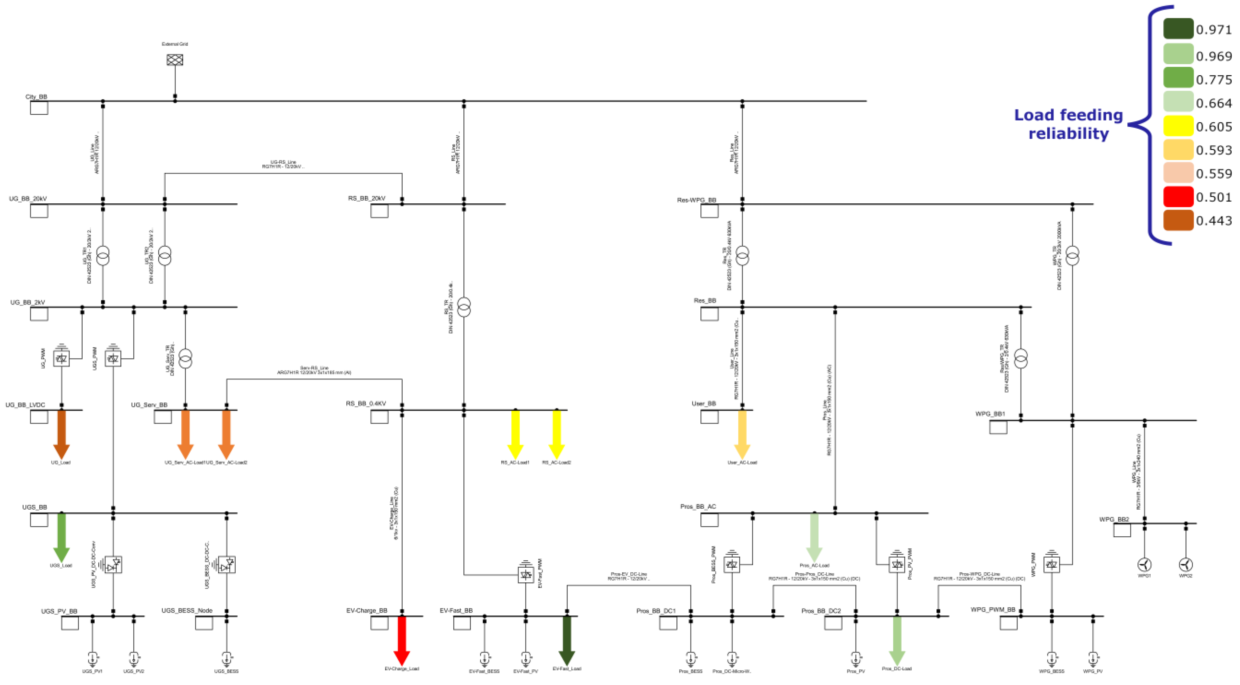
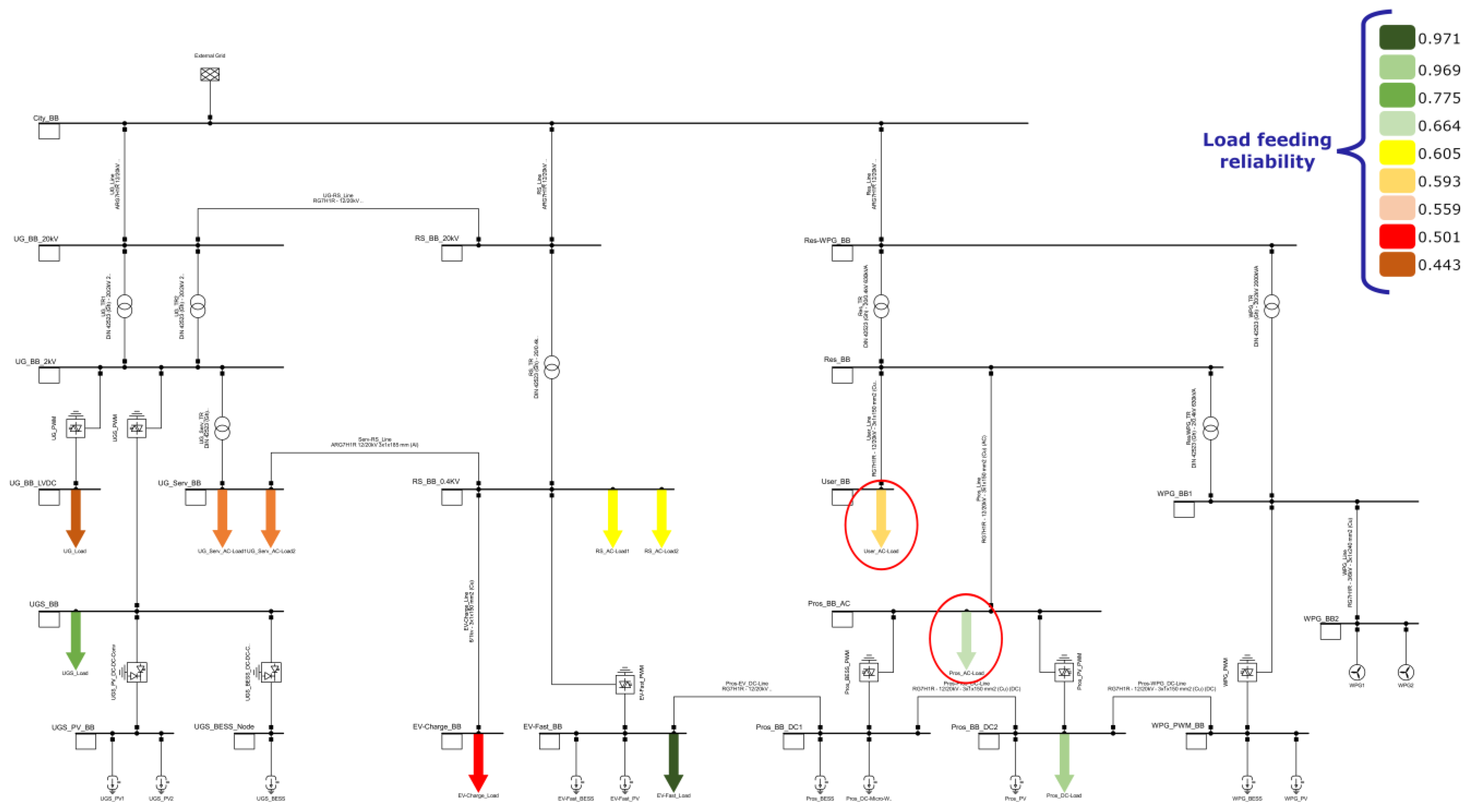
• The proposal and calculation of the “load feeding reliability” index for each consuming unit of the power system under investigation.

It can provide a significant contribution for the definition of solutions and strategies able to increase service continuity identifying unreliable systems or load feeding paths.

In this paper, Section 2 is dedicated to the details and description of the proposed RPM. In Section 3, the synthetic hybrid power system used to study the effectiveness of the model is presented. A case study and the obtained reliability assessment are reported in Section 4.

2. Reliability Models of Power Systems Components

In Section 2.1, the general reliability model is presented, and in next subsections details about power systems lines, transformers, circuit breakers, converters and renewables plants are described.

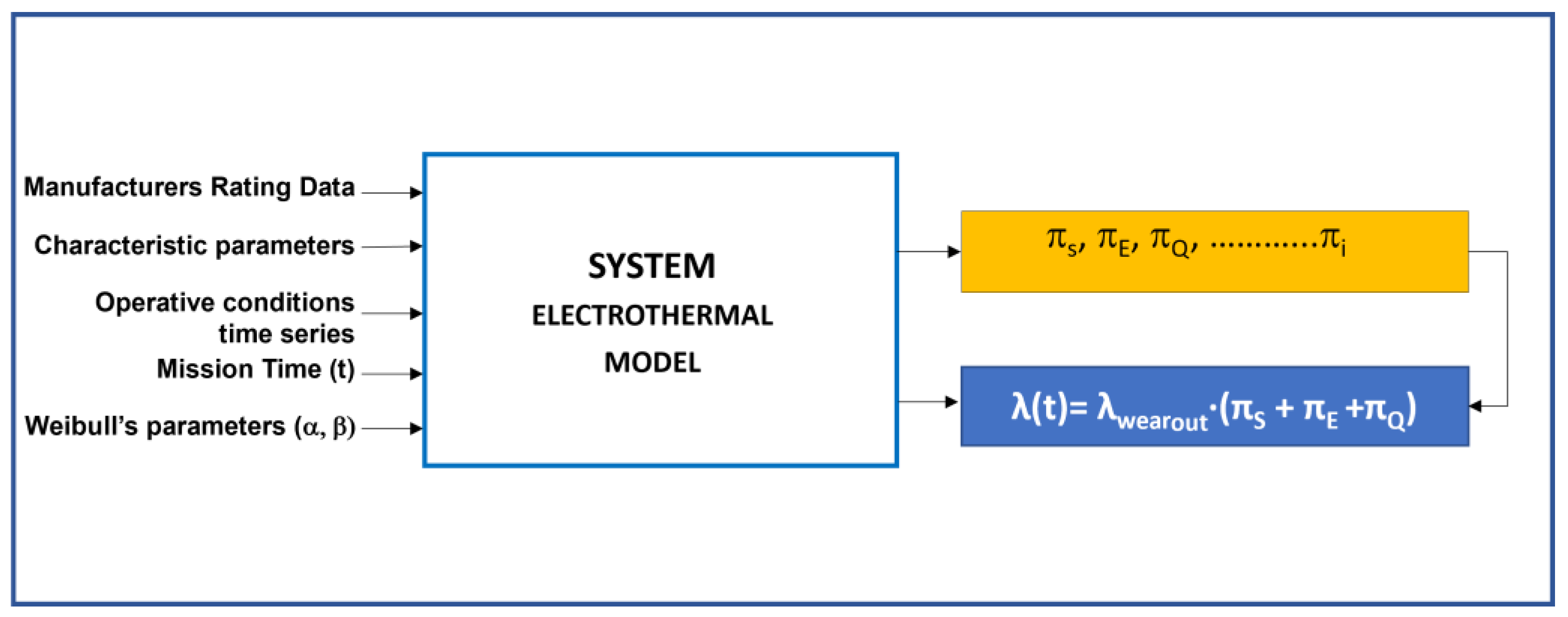
2.1. Reliability Model

The process to develop the reliability model for a grid component is graphically schematized in Figure 1. In the beginning, the attention is focused on each device or component of the investigated power system.

Necessary inputs are the manufacturer rating data, characteristic parameters of the component under modeling, operative conditions time series, mission time information, and Weibull aging parameters for each component. In addition, a single-line diagram about the grid or microgrid where the device under test is connected is required. The core of the model is constituted by the device electro-thermal equivalent circuit.

Component-level simulations and load flow analyses of the whole power system are carried out considering operative conditions by time series of the input data (ambient temperature, irradiance, wind speed of the installation sites) and their uncertainties.

As in MIL-HDBK-217F [3] and in other available RPMs, stress impacts are evaluated by π_i factors: thermal (π_S), environmental (π_E) and quality stresses (π_Q).

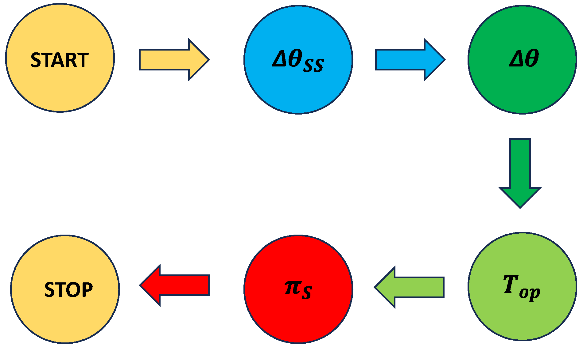
2.1.1. Thermal Stress π_S

Thermal stress π_S is determined by temperature variations impacting materials properties and thus causing losses in the functioning mode. This stress is associated with overloading and overtemperature conditions, and with thermal cycles to which the system is subjected during operative modes.

The π_S factor is evaluated calculating the component temperature in relation to the climatic time series (inputs) and the operating conditions (simulations).

This temperature is obtained by the formula reported in Equation (1).

$$T_{op}=T_{amb}+\mathsf{\Delta }\theta$$

(1)

where Δθ is the device temperature rise, and it is evaluated according to Equation (2).

$$\mathsf{\Delta }\theta =\mathsf{\Delta }{\theta }_{ss}\left(1-e^{\frac{-t}{T}}\right)$$

(2)

where the following are defined:

• T is the thermal constant;
• t is the mission time;
• Δθ_ss is the steady state temperature rise.

Δθ can be calculated considering the energy conservation low (Equation (3)) by some mathematical steps, as detailed in [18].

$${\dot{Q}}_{in}+{\dot{Q}}_{gen}=\mathsf{\Delta }{\dot{Q}}_{stor}+{\dot{Q}}_{out}$$

(3)

where the following are defined:

• ${\dot{Q}}_{in}$ is the heat flow rate due to the solar radiation on the specific device/system;
• ${\dot{Q}}_{gen}$ is the heat generation rate in the system/line due to power losses;
• ${\dot{Q}}_{out}$ is the dissipated heat flow rate;
• $\mathsf{\Delta }{\dot{Q}}_{stor}$ is the heat accumulation rate in the device/system, responsible for the temperature increasing.

Knowledge of the operative temperature T_op (Equation (1)) for each functioning condition permits the calculation of the thermal cycles to which the system/line is subjected. More in detail, the number of thermal cycles occurring in an annual time interval is considered and the maximum temperature of these thermal cycles is identified. Finally, a modified formula of the Norris–Landzberg model, which evaluates the fatigue mechanism acceleration due to thermal variations, is applied to calculate the thermal stress π_S value. It is presented in the FIDES RPM [5] and it is reported in Equation (4).

$${\pi }_S=\left(\frac{12·N_{annual\_cycl}}{t_{annual}}\right)·{\left(\frac{{∆T}_{cycl}}{T_0}\right)}^{{\mathit{m}}_{\mathit{B}}}·\mathrm{e}\mathrm{x}\mathrm{p}\left[1414·\left(\frac{1}{T_0+\Delta T_0}-\frac{1}{T_{\mathrm{m}\mathrm{a}\mathrm{x}\_cycl}}\right)\right]$$

(4)

where the following are defined:

• N_{annual_cycl} is the number of thermal cycles in an annual time interval;
• t_annual is the annual number of hours;
• m_B is the fatigue coefficient [5];
• ΔT_cycl is the maximum thermal cycle amplitude (°K);
• T_{max_cycl} is the maximum temperature in thermal cycles (°K);
• T₀ is the reference temperature value (°K);
• ΔT₀ is the reference thermal range (°K).

2.1.2. Environmental Stress π_E

The π_E factor is determined by the stressing agents related to the device environmental conditions due to its installation site. In addition to environment conditions defined by mentioned RPMs,

Table 1. Environmental conditions of power system components.

Environment	Description
Ground, G	non-mobile environment, characterized by uncontrolled temperature and humidity
Ground, Benign GB	non-mobile environment, easily accessible for maintenance, characterized by controlled temperature and humidity
Ground, Fixed GF	moderately controlled environment with an adequate cooling system and possible installation in unheated buildings
Ground, Solar GS	uncontrolled environment exposed to solar radiation and atmospheric agents
Ground, Saline GA	uncontrolled environment characterized by dust and salt and exposed to solar radiation and atmospheric agents
Ground, Unsheltered GU	environment in which equipment is unprotected, exposed to weather conditions and equipment immersed in salt water
Underwater U	underwater environment

describes environment characterized by solar radiation, salt and dust agents.

2.1.3. Quality Stress π_Q

Another stressing factor is related to systems/devices qualitative level. In fact, the ability to perform a specified functioning modes for a specified period of time is also influenced by materials constituting the considered system/device and its production process. In the proposed model, this kind of stress is taken into account by the π_Q factor.

In analogy to MIL-HDBK-217F [3], the components can be characterized by a standardized or non-standardized (commercial product) quality level.

2.1.4. Aging Phenomena λ_{wear_out}

The proposed reliability model also aims to include wear-out phenomena affecting devices performances. Studies on different components demonstrated the Weibull distribution suitability to model such phenomena [14].

The failure rate function of the two-parameter Weibull distribution is reported in Equation (5):

$${\lambda }_{wear\_out}(t)=\frac{\beta }{\alpha }{\left(\frac{t}{\alpha }\right)}^{\beta -1}$$

(5)

where the following are defined:

• β is the shape factor;
• α is the scale factor defined as the time at which 63.2% of components have failed.

2.1.5. Failure Rate λ and Mean Time between Failure

The proposed reliability model (Figure 1) allows user to represent each component or system by means of the failure rate λ [h⁻¹] determined by the joint action of the stressing agents (thermal, environmental, etc.) and the aging phenomena, as schematically reported in the following Equation (6).

$$\lambda ={\lambda }_{wear\_out}·\sum _i{\pi }_i={\lambda }_{wea{r}_{out}}·\left({\pi }_S+{\pi }_E+{\pi }_Q\right)$$

(6)

Another significant index for evaluating devices/systems reliability is the Mean Time Between Failure [h]. It expresses how reliable a device/system results. The Mean Time Between Failure (MTBF) formula is reported in Equation (7).

$$MTBF=\frac{1}{\lambda }$$

(7)

The described model is implemented in an open-source software package (Version 1.0) developed with Python Programming Language.

In the following paragraphs, details about the proposed RPM for different grid systems and devices are reported.

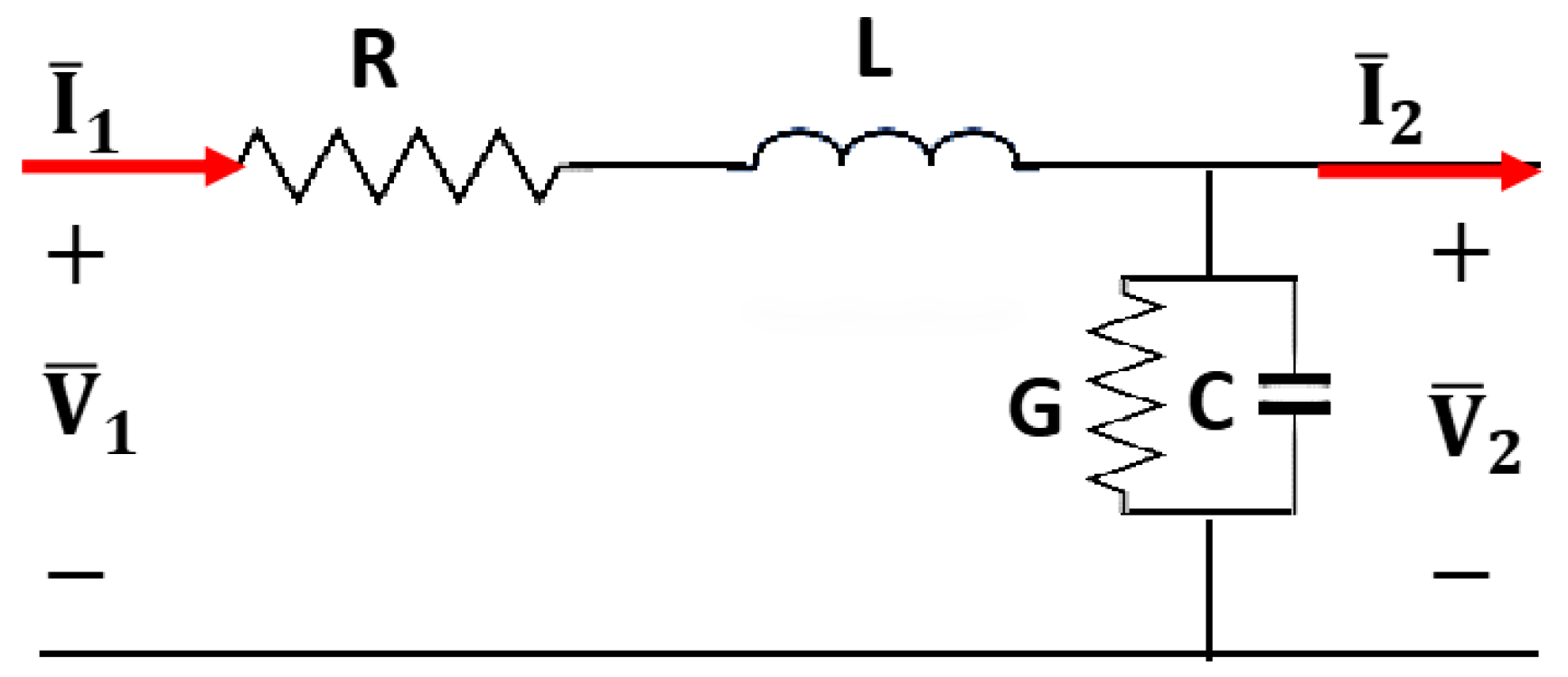
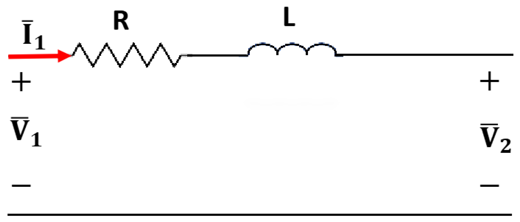
2.2. Overhead Distribution Line Reliability Model

Distribution power systems are characterized by medium-voltage (MV) and low-voltage (LV) overhead and underground lines. In order to develop the reliability model of a power line, the attention is focused on the core of the cable comprising the conductor wrapped in the dielectric layer. In detail, the power distribution systems are characterized by short lines to ensure low-voltage drops. This aspect allows user to model its behavior using lumped parameter equivalent circuit, as reported in Figure 2.

It comprises a series impedance and a parallel admittance; it neglects propagative effects. The reported model can be further simplified in case of MV short lines (Figure 3).

It is suitable for both the AC and DC lines of the hybrid grid. In operating conditions, each line is subjected to thermal stress related to overtemperature, thermal shocks due to overload events and thermal cycles.

In detail, the thermal stress factor π_s is evaluated starting from the energy conservation law and repeating the process described above to determine the line temperature rise for each operative condition, also considering climatic and environmental aspects. The mathematical steps necessary to calculate the line temperature rise are detailed elsewhere [18]. Δθ evaluation allows us to calculate the thermal stress π_S impacting on the grid lines, as schematically reported in Figure 4.

Environmental aspects concerning each overhead line are investigated considering the characteristics of its installation site to quantify the relative π_E factor, according to the environmental conditions reported in Table 1.

In addition, line material properties are analyzed to evaluate the quality factor π_Q.

Ageing phenomena are taken into account by the mentioned two-parameter Weibull distribution (Equation (5)). In detail, the implemented software permits us to fill in the scale and shape parameters [14] to calculate the line failure rate λ_line as in Equation (8).

$${\lambda }_{line}={\lambda }_{wear\_out\_line}·\sum _i{\pi }_{i\_line}={\lambda }_{wea{r}_{out\_line}}·\left({\pi }_{S\_line}+{\pi }_{E\_line}+{\pi }_{Q\_line}\right)$$

(8)

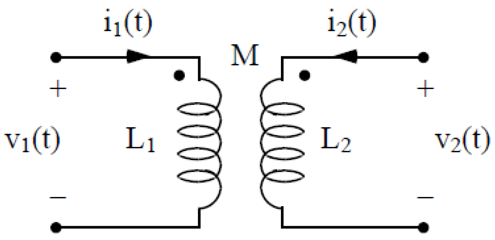
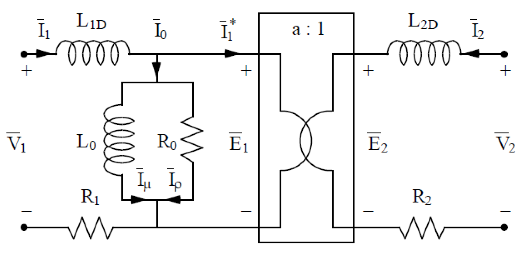
2.3. Power Transformer Reliability Model

Power systems are characterized by power transformers, static electrical machines installed in the primary and secondary substations for the transformation of high voltage (HV) into MV and MV into LV, respectively.

The power transformer represents a critical element of the electrical networks. Different failure phenomena can affect its correct behavior, not only impacting service continuity of various customers, but also causing extensive damage (oil leakage, explosions, fires).

In detail, the main subsystems of a power transformer consist of windings, core and cooling components.

The copper or aluminum windings are insulated and organized in turns. The core comprises a lamellar pack in high permeability ferromagnetic material.

Three-phase transformers are made with a single core characterized by three primary and secondary phases connected in a star or delta configuration according to different connection schemes.

The cooling system is based on the thermal inertia of the oil in the case of oil-cooled transformers, while it consists of tangential fans in the resin transformers.

The proposed reliability model accepts the transformer rate data (apparent power and percentage of losses in copper and iron), the environmental and climatic conditions of the installation site and the single-line diagram of the network to which the transformer is connected.

In Figure 5, the equivalent circuit of a single-phase transformer is shown [19], consisting of two windings and the core. The high- and low-voltage coils wound on the ferromagnetic support constitute two mutually coupled circuits, where L₁ and L₂ represent, respectively, the self-inductance in the primary and the secondary sides of the transformer and M represents the mutual inductance.

The imperfect coupling is modeled by adding the magnetizing inductance L₀ in parallel to the primary of the transformer, as reported in the equivalent circuit of Figure 6.

There are magnetic hysteresis and eddy currents losses. The magnetic hysteresis implies that part of the energy supplied for the magnetization of the core remains stored in the core itself during the demagnetization phase, increasing power losses. Eddy currents, on the other hand, are due to currents that circulate in the core of the transformer since it is constituted is a good electrical conductor.

A model of the transformer representing the real behavior can be obtained taking into account phenomena determining ferromagnetic core losses. They are due to magnetic hysteresis and eddy currents and lead to increase in the transformer temperature.

These losses are modeled by inserting resistance R₀ in parallel to the magnetization inductance L₀. Since the non-ideality of the iron in the core, not all the magnetic flux lines generated in the two windings are internal to the iron: part of the flow is dispersed. This phenomenon is modeled by inserting a longitudinal inductance to the primary (L_1D) and one to the secondary (L_2D) of the transformer. Furthermore, two resistors (R₁ and R₂) represent copper losses due to primary and secondary windings (Figure 6).

Numerical values of these equivalent circuit parameters are calculated from the transformer rating data. In detail, manufacturers provide the iron (Equation (9)) and copper (Equation (10)) losses as a percentage of the apparent power of the transformer A_n (further rating data of the transformer). In detail, from the formula of copper losses (Equation (10)), the value of the equivalent secondary resistance of each phase R_eq is calculated.

$$P_{Fe\%}=\frac{P_{Fe}}{A_n}·100$$

(9)

$$P_{cc\%}=\frac{P_{cc}}{A_n}·100=\frac{3 R_{eq }{\overline{I_{Sn}}}^2}{A_n}·100=\frac{3 R_{eq }{A}_n}{{\overline{V_{Sn}}}^2}·100$$

(10)

where the following are defined:

• I_Sn is the nominal secondary current;
• V_Sn is the nominal secondary voltage.

The R_eq knowledge permits the calculation of losses in the transformer windings in real operating conditions.

For the purposes of assessing reliability using the proposed methodology, the transformer is considered a system consisting of the connection between the three subsystems: core, cooling and windings. This logical series connection implies that a fault condition in one of the three subsystems can affect the functionality of the entire transformer. In the rest of this paragraph, attention is focused on the factors affecting the mentioned transformer subsystems.

With reference to windings, thermal phenomena affecting both copper conductors and insulation surrounding them must be considered.

According to what was previously proposed, the information provided by the input data series and the rating data allows the calculation of the winding resistances in the considered operating conditions.

At this point, proceeding in a similar manner to what is reported for overhead lines, the overtemperature and, therefore, the operating temperature for each operating condition is calculated. Using the Norris–Landzberg model, the authors obtain a quantitative evaluation of the thermal stress π_{s_win}, which also takes into account the cyclic thermal phenomena acting on the transformer windings.

The π_{S_core} factor is also calculated (from input and rating data) considering the thermal resistance of the ferromagnetic material of the core.

Downstream of this calculation, the identification of the thermal cycles to which the core is subjected allows the evaluation of the π_{S_core} factor.

Furthermore, the thermal phenomena involving the cooling medium of the transformer should be considered.

The factor π_{S_cool} is calculated using the following equation:

$${\pi }_{s\_cool}=e^{{\left(\frac{1}{T_1}-\frac{1}{T_2}\right)B}_T}$$

(11)

where the following are defined:

• B_T is a constant [20];
• T₁ is the temperature value at t₁;
• T₂ is the temperature value at t₂.

The constant B_T is calculated by Equation (12).

$$B_T=\frac{\mathrm{l}\mathrm{n}\left(\frac{1}{2}\right)}{\left(\frac{1}{T_1}-\frac{1}{T_2}\right)}$$

(12)

It is known that above 90 °C, the life of the transformer is halved [20] for every 10 °C increase in temperature.

The π_{E_t} and π_{Q_t} factors are determined as described above. In detail, the transformer can be installed in a ground-type environment (also ground benign, fixed or saline). Therefore, the solar radiation effect and salty environment must be appropriately considered in the environmental factor evaluation.

Furthermore, transformers are characterized by subsystems which, in accordance with the sector regulations, must ensure specific quality levels impacting the ${\pi }_{Q\_t}$ factor.

Finally, it is necessary to consider the degradation of windings materials, core and cooling system appropriately inserting the scale factor and the shape factor in the Weibull distribution equation of the λ_{wear_out} in order to determine λ_{w_win}, λ_{w_core} and λ_{w_cool}.

At this point, the transformer has been modeled from the reliability point of view and, therefore, simple mathematical calculations make it possible to obtain the value of the λ_TRAF by means of Equation (13).

$${\lambda }_{TRAF}=\left({\lambda }_{w\_win}+{\lambda }_{w\_core}+{\lambda }_{w\_cool}\right)·\left({\pi }_{s\_win}+{\pi }_{s\_core}+{\pi }_{s_{cool}}+{\pi }_{E\_t}+{\pi }_{Q\_t}\right)$$

(13)

2.4. Circuit Breaker Reliability Model

Traditionally, circuit breakers (CBs) are electromechanical switches [21] able to open circuits to protect them in case of overcurrent/overvoltage conditions. Recently, attention has been focused on electronic devices realized by solid-state components [22].

Regarding oil CBs, the correct behavior is determined by the correct functioning of conductors, insulators, cooling medium (oil) and mobile contacts.

As above reported, it is possible to evaluate the CB stresses. In detail, starting from the input time series, it is possible to evaluate the thermal cycles and, therefore, the thermal stress factors affecting the conductors, the insulators, the cooling medium and the mobile contact.

According to the CB installation site, it is possible to evaluate the type of environment and the relative stress π_{E_CB}. The quality factor π_{Q_CB}, on the other hand, is determined by CB materials.

A further step is represented by evaluating the effects of aging on the different CB components.

Considering the form and scale factors related to the Weibull-type distributions that characterize the degradation of the materials of the conductors (α_cond, β_cond), the insulators (α_ins, β_ins), the moving contact (α_cont, β_cont) and the cooling medium (α_cool, β_cool), the failure rate λ_{w_CB} is determined, as below reported (Equation (14).

$${\lambda }_{w\_CB}=\left({\lambda }_{{w\_}_{cond}}+{\lambda }_{{w\_}_{is}}+{\lambda }_{{w\_}_{cool}}+{\lambda }_{{w\_}_{cont}}\right)$$

(14)

where the following are defined:

• λ_{w_cond} is the wear-out failure rate for CB conductors;
• λ_{w_ins} is the wear-out failure rate for CB insulators;
• λ_{w_cool} is the wear-out failure rate for the CB cooling medium;
• λ_{w_cont} is the wear-out failure rate for the CB moving contact.

In conclusion, the overall failure rate of oil CB can be calculated using Equation (15).

$${\lambda }_{C{B}_{oil}}=\left({\lambda }_{{w\_}_{cond}}+{\lambda }_{{w\_}_{ins}}+{\lambda }_{{w\_}_{cool}}+{\lambda }_{{w\_}_{cont}}\right)·\left({\pi }_{s_{\_cond}}{+{\pi }_{{si}_{ins}}+{\pi }_{{s\mathrm{e}}_{\_ins}}+{\pi }_{s_{\_cool}}+{\pi }_{s_{\_cont}}+\pi }_{E_{CB}}+{\pi }_{Q\_CB}\right)$$

(15)

On the other hand, if the CB is made using solid-state components, the main topologies proposed in the literature are characterized by Insulated Gate Bipolar Transistors (IGBTs), Gate-Commutated Turn-off (GCT) or Gate Turn-Off (GTO), diodes, capacitors and inductors. Some examples of topologies of such CBs are reported in the literature both for MV AC networks [22] and for MV DC networks [21].

In this case, the reliability model can be implemented by considering switching, capacitors and magnetic elements stresses according to their specific topologies.

The effect of thermal stresses incident on this type of device is analyzed as detailed in Section 2.5. Environmental and quality factors are evaluated as reported above. The impact of aging phenomena on CB reliability is evaluated by IGBTs (GCTs, GTOs) capacitive and magnetic devices Weibull parameters.

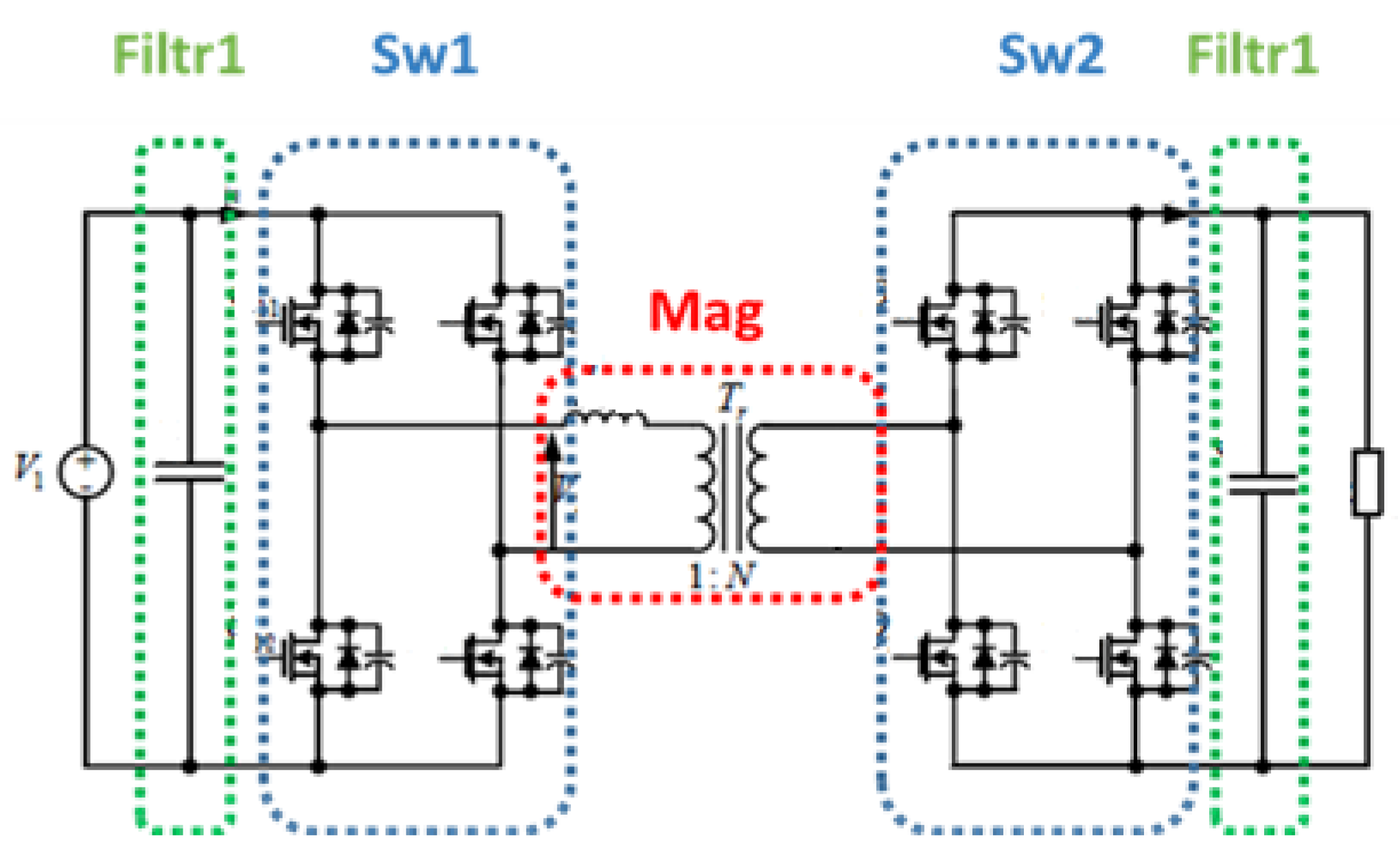
2.5. DC/AC and DC/DC Converters Reliability Model

DC/AC and DC/DC converters, used as interfaces to connect DC equipment to AC or DC buses, respectively, are switching systems. They can be unidirectional or bidirectional, transformerless or transformer-equipped. These converters are based on switching devices such as IGBTs or Metal–Oxide–Semiconductor Field-Effect Transistors (MOSFETs).

As regards the equivalent model of the converter, State-Space Averaging or Pulse Width Modulation (PWM) models can be applied for the different topological solutions of DC/DC and DC/AC converters [23,24]. Given the large number of topological solutions that can be adopted and since the converter models are described in various publications, this paper omits the converter model and refers to the literature in the sector [23,25,26].

For the purpose of this study, it is necessary to develop an electro-thermal model that takes into account the influence of temperature and thermal cycles on the parameters of the electronic devices of converters.

Despite the limited information available through the datasheet provided by the manufacturers, the determination of electro-thermal models of these devices can be obtained considering device parameters dependence on temperature and using the iterative approach reported elsewhere [27].

Starting from the value of the parameters at room temperature, the iterative algorithm proceeds, through a subsequent refinement process, to calculate the value of the device parameters at different temperatures. Switching converter performance and reliability deeply depends on switching devices. It should be underlined that, in MOSFETs datasheets, the manufacturers report the graphs representing the Drain-Source resistance R_DS, the threshold voltage V_th and the transconductance g_fs dependence on temperature.

Input time series are used to identify the maximum ambient temperature value T_{a_MAX}. Graphs necessary to calculate the MOSFET characteristic parameters at the reference temperature of 25 °C are acquired from the datasheet. Then, the calculation of the conduction and switching losses of the MOSFET is carried out taking advantage of the equivalent circuit of the converter and the operative conditions. In this way, it is possible to calculate the value of the maximum junction temperature T_{j_MAX} of the MOSFET and the characteristics of the thermal cycle to which the device is subjected. In this case, values of characteristic parameters (R_DS, V_th, g_fs) depending on the junction temperature can be refined. If the iterative process shows the achievement of T_{j_MAX} values higher than the threshold, it is necessary to equip the MOSFET with a suitable heatsink.

The obtained T_{j_MAX} values permit to calculate the MOSFET temperature rise, and then it is possible to apply the Norris–Landzberg model in order to quantitatively determine the thermal stress π_{S_sw}. In a similar manner, the iterative approach can be applied to other converter devices, thus obtaining the relative thermal stresses values.

The whole converter calculation can be carried out considering its topological solution. As an example, the following figure reports a dual active bridge (DAB) converter.

As shown in Figure 7, such a converter comprises an input filter and an output one, a switching stage and a magnetic section.

Failure rates relative to the mentioned converter section are reported in Equations (16)–(20).

$${\lambda }_{Filtr1}={\lambda }_{w\_C}· \left({\pi }_{s_{Filtr1}+}{\pi }_{E\_s_{Filtr1}}+{\pi }_{Q\_s_{Filtr1}}\right)$$

(16)

$${\lambda }_{Filtr2}={\lambda }_{w\_C}· \left({\pi }_{s_{Filtr2}+}{\pi }_{E\_Filtr2}+{\pi }_{Q\_Filtr2}\right)$$

(17)

$${\lambda }_{Sw1}={\lambda }_{w\_Sw}· \left({\pi }_{sSw1 }{+\pi }_{E\_Sw1 }+{\pi }_{Q\_Sw1}\right)$$

(18)

$${\lambda }_{Sw2}={\lambda }_{w\_Sw}· \left({\pi }_{sSw2}{+\pi }_{E\_Sw2 }+{\pi }_{Q\_Sw2}\right)$$

(19)

$${ \lambda }_{Mag}={\lambda }_{w\_L}· \left({\pi }_{sL }{+\pi }_{E\_L }+{\pi }_{Q\_L}\right)$$

(20)

where λ_{w_C}, λ_{w_Sw} and λ_{w_L} are wear-out failure rates of capacitors, switching and magnetic components obtained using the relative scale and shape parameters.

The failure rate of the whole converter will be obtainable by considering a series-type logical connection between the considered sections.

Such a series connection among converter devices determines its functionality only in the case of operation of all its sections. The converter failure rate can be calculated as the sum of the different devices failure rates as in Equation (21).

$${\lambda }_S(t)=\sum _{i=1}^N{\lambda }_i(t)$$

(21)

Substituting Equations (16)–(20) in Equation (21), the formula of the converter failure rate is obtained.

This method can be applied to any other converter topological solution.

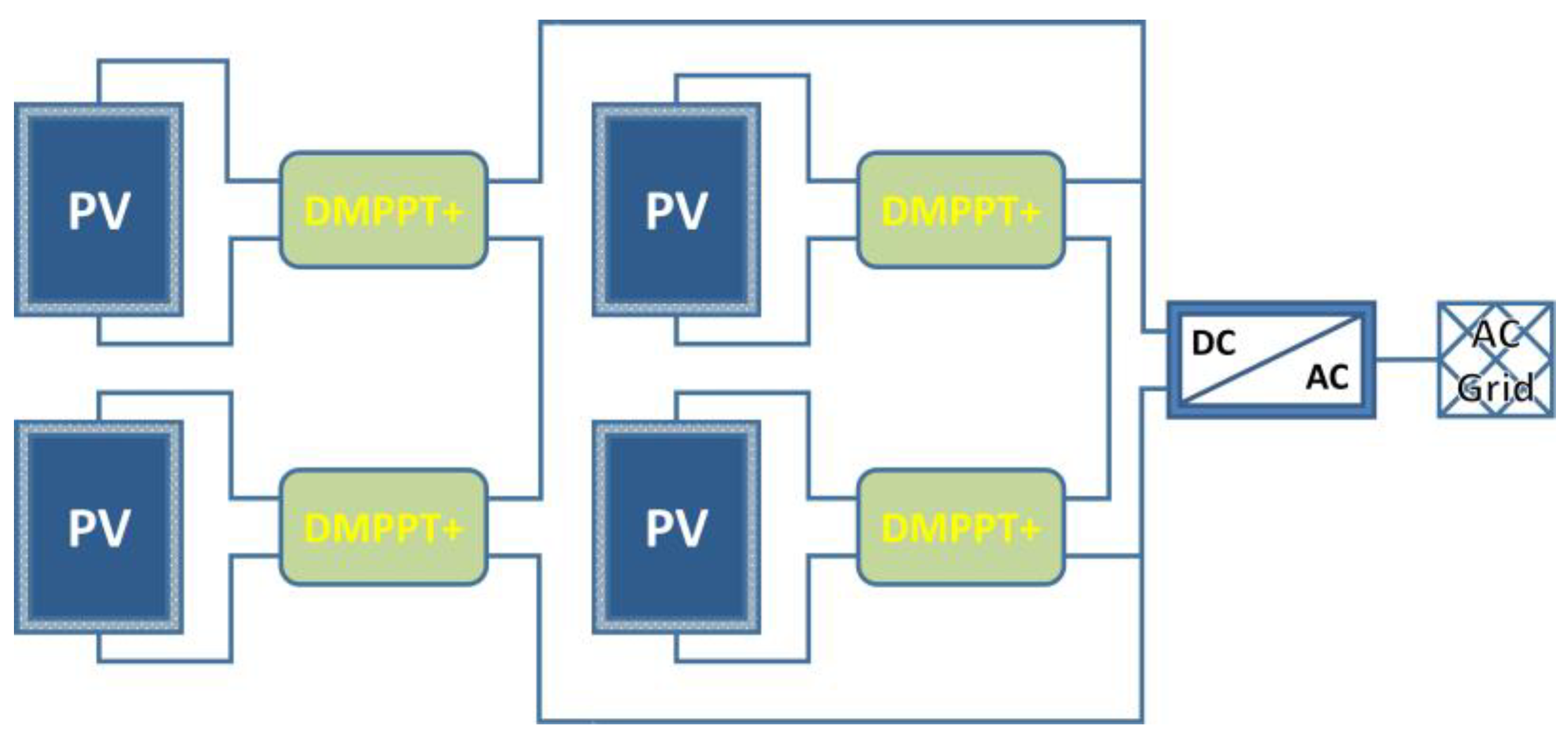
2.6. Renewables Plants Reliability Model

The evaluation of the performance of renewable sources in terms of reliability represents a crucial issue especially in view of the massive introduction and connection of these plants to the national grid. In this paper, the reliability assessment of photovoltaic (PV) and wind generators is carried out.

In particular, PV degradation can be modeled only by deeply understanding the mechanisms and processes of cells at the microscopic level and regarding module encapsulant and film.

However, it must be underlined that PV generators are connected to AC or DC buses by means of DC/AC or DC/DC converters.

The logical connection between the set of PV modules and the conversion section is the series type, and thus, the system will only be operational in cases where both generation and conversion sections work properly.

Field data from PV systems demonstrate that converters are the least reliable part of PV plants [28].

Given the lower reliability of the conversion apparatus than that of the PV module one, it is necessary to proceed with the reliability modeling of the DC/DC and DC/AC converters (Figure 8), considering the following:

• PV generators can be onboard-equipped with Distributed Maximum Power Point Tracking (DMPPT) converters;
• The operating temperature of DMPPT converters depends on the weather and climatic conditions of the installation site, on the location on the back of the PV module and on their functioning conditions.

The reliability model of such converters results is similar to that presented in Section 2.5.

In the case of generators equipped with DMPPT+ converters, the failure rate can be calculated as in Equation (22).

$${\lambda }_{PVgen}\approx {{\lambda }_{DMPPT+}+\lambda }_{conv}$$

(22)

The PV plant failure rate λ_{PV_plant} is obtained considering series/parallel connections among different arrays and the failure rate relative to the plant DC/AC (or DC/DC) converter, as in Equation (23):

$${\lambda }_{PV\_plant}\approx {\lambda }_{ALL\_PV\_gen}+{\lambda }_{PV\_conv}$$

(23)

Figure 8. PV plant with DMPPT and inverter interface.

Figure 8. PV plant with DMPPT and inverter interface.

In a similar way, the reliability of the system consisting of a wind generator and interface circuit can be calculated. In detail, the interface converter consists of an AC/DC converter in case of an on-shore wind generator, while it is a DC/DC converter in case of an off-shore wind turbine.

The failure rate for wind generators, λ_windgen, will be approximated by the following formula:

$${\lambda }_{windgen}\approx {\lambda }_{wind\_conv}$$

(24)

where λ_{wind_conv} is the failure rate of the wind generator converter.

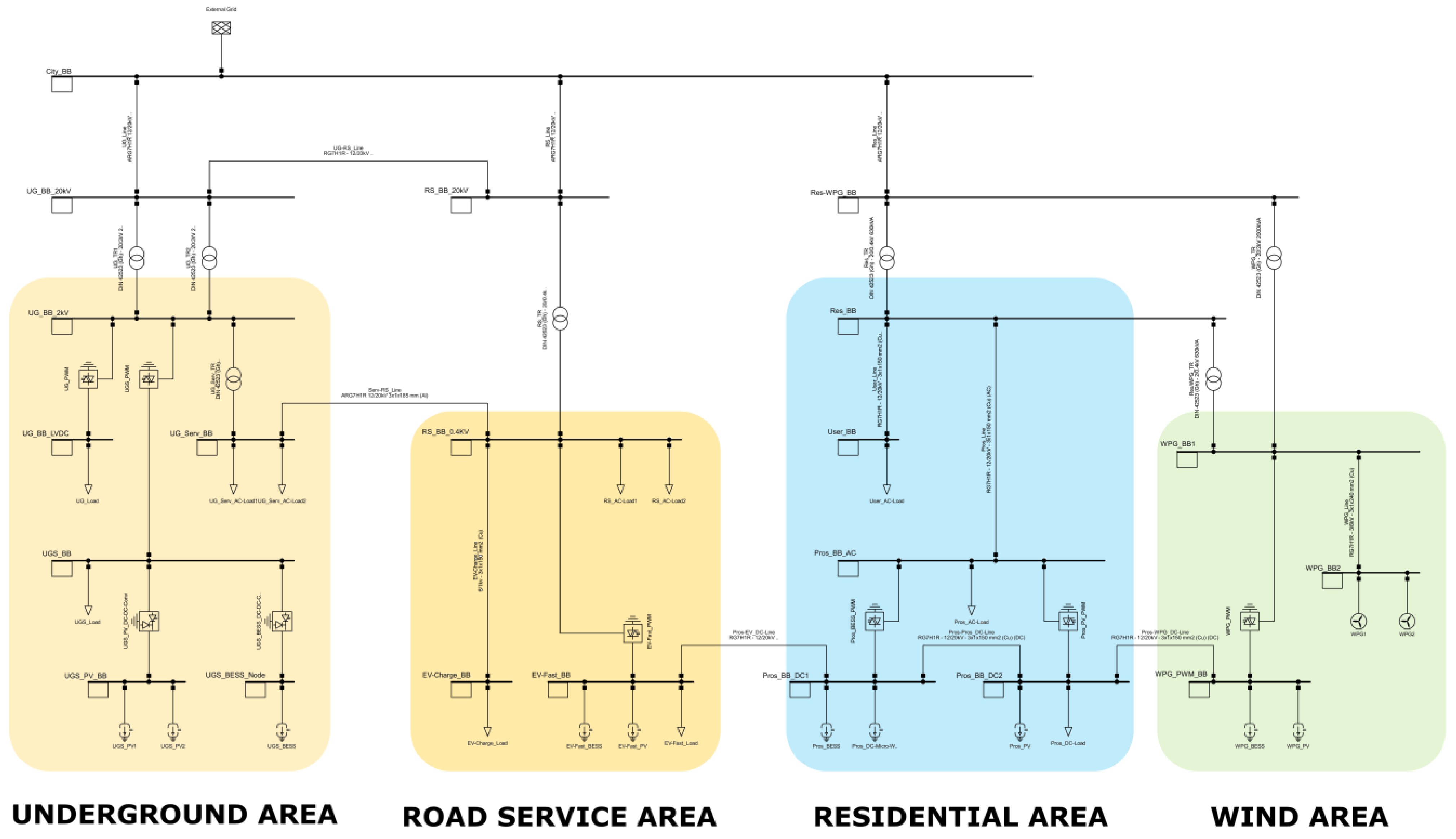
3. Benchmark Synthetic Grid and Reliability Indices

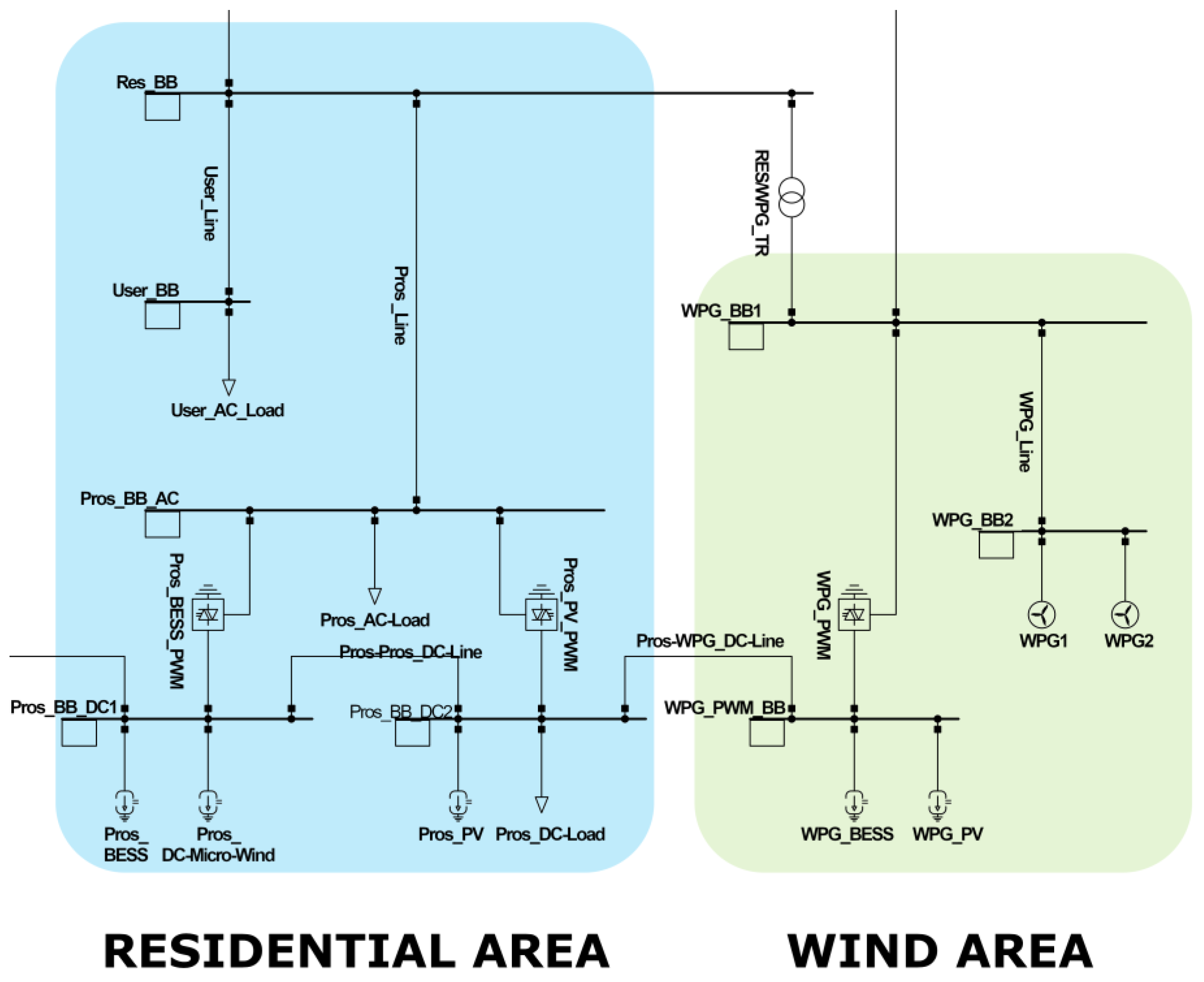
In the previous section, the general and specific reliability models are presented for different grid components. The reported process and formulas allow the calculation of the failure rates for each power system device. In the following, a case study is analyzed to show how the reliability assessment can be carried out for a radial and/or meshed grid.

The attention is here focused on hybrid (AC, DC) power systems, since the availability of DC native generators (PV, fuel cell), storage (Li-ion batteries, flow batteries) and loads (servers, cooling, heating systems) is increasing with consequent realization of DC micro-grids connected to the AC main grid through power converters [26]. As hybrid (AC, DC) grids will play a key role in the future power grid, a hybrid urban grid benchmark model has been defined as a synthetic power system for reliability studies (Figure 9).

The grid comprises four specific areas:

• A residential area;
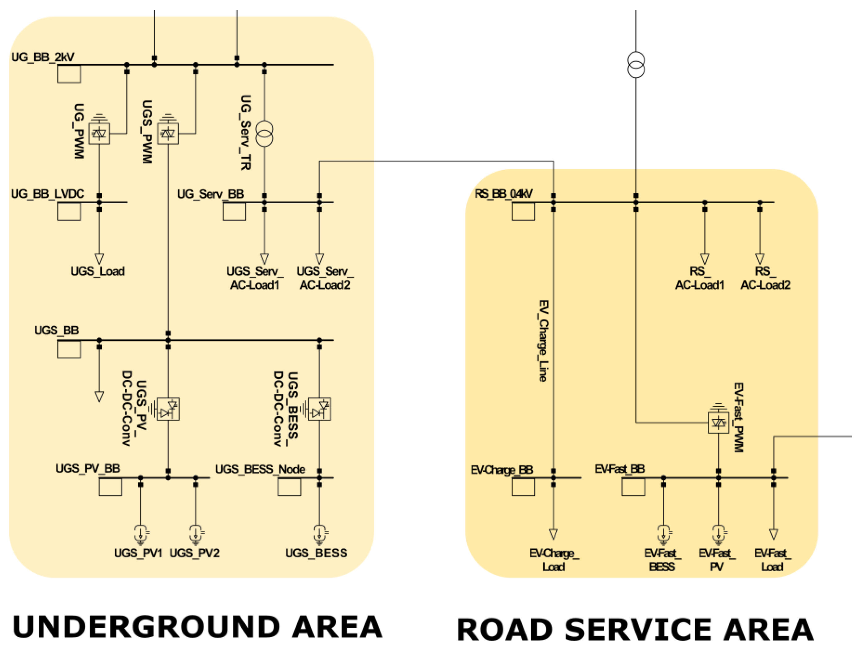
• An underground transportation area;
• Electric vehicle charging (EVC) stations and a public lighting (road service) area;
• A wind generation area.

The underground area, shown in Figure 10, contains loads and needed services units. Figure 10 also reports the road service area including public lighting and EVC stations.

Figure 11 reports the residential area including domestic consumers and prosumers, and the wind area, representative of a suburban zone characterized by a great usable surface with mini wind installations directly connected to the AC distribution network, PV plants and storage systems connected to DC busbars.

Detailed information on loads, distributed generation and energy storage for the proposed grid is summarized in

Table 2. Rated parameters of loads, distributed generators and storage systems.

Grid Sector	Element Name	Element Type	Rating Data
Underground Area	UG_Load	DC Load	800 kW
	UGS_Load	DC Load	800 kW
	UG_Serv_AC-Load1	AC Load	222 kVA (200 kW)
	UG_Serv_AC-Load2	AC Load	222 kVA (200 kW)
	UGS_PV1	PV	50 kW
	UGS_PV2	PV	50 kW
	UGS_BESS	Storage	300 kW–600 kWh
Road Service Area	RS_AC-Load1	AC Load	111 kVA (100 kW)
	RS_AC-Load2	AC Load	111 kVA (100 kW)
	EV-Charge_Load	AC Load	44 kVA (40 kW)
	EV-Fast_Load	DC Load	300 kW
	EV-Fast_PV	PV	50 kW
	EV-Fast_BESS	Storage	200 kW–400 kWh
Residential Area	User_AC-Load	AC Load	278 kVA (250 kW)
	Pros_AC-Load	AC Load	244 kVA (220 kW)
	Pros_DC-Load	DC Load	50 kW
	Pros_PV	PV	100 kW
	Pros DC-Micro-Wind	DC Wind Power Generator	20 kW
	Pros_BESS	Storage	200 kW–400 kWh
Wind Area	WPG1	AC Wind Power Generator	200 kVA
	WPG2	AC Wind Power Generator	200 kVA
	WPG_PV	PV	100 11 kW
	WPG_BESS	Storage	400 kW–600 kWh

.

Generally, the failure rate of a system constituted by subsystems can be evaluated by analyzing the logical series/parallel connections among its subsystems.

The application of Equation (25) (for series configurations) and Equation (26) (for parallel configurations) permits us to obtain the system failure rates.

Two or more units are series connected if their proper functioning mode is assured only in the case where each unit works correctly.

The parallel structure system fails only when every one of its units fails.

The following formulas report failure rates for series (λ_s) and parallel (λ_p) connected systems, respectively:

$${\lambda }_S(t)={\sum }_{i=1}^N{\lambda }_i(t)$$

(25)

$$\frac{1}{{\lambda }_p(t)}={\sum }_{i=1}^N\frac{1}{{\lambda }_i(t)}$$

(26)

where λ_i is the ith unit failure rate.

The same approach must be applied to power systems, but their complexity makes difficult the identification of series/parallel connected sections of the grid.

Furthermore, some loads can be supplied by different sources, and some others are connected in hybrid series/parallel connections. In this context, the whole grid failure rate value is not meaningful since it provides “cumulative” information unable to indicate low-reliability equipment and the relative collocation in the grid. In the authors’ opinion, the reliability assessment has to evaluate not only each device/system failure rate, but also the reliability of load supply. In this case, all possible power paths able to source each grid load are identified by investigating the complex networks through graphs theory. More in detail, this operation is conducted by using the Python NetworkX module. Figure 12 shows the graph related to the UGS_Load in the underground area.

This graph includes traditional sources, renewables generators and storage systems able to supply the UGS_Load.

The “load feeding reliability“ index is defined as the failure rate evaluation of all possible paths supplying a specific consumption unit, taking into account the failure rates of all generation nodes of these paths also considering the present series/parallel or hybrid connections among them.

This index provide meaningful information since its low value is representative of an alerting context for the Transmission System Operator (TSO), Distribution System Operator (DSO), prosumers and also for the load customer. In this case, solutions could be adopted to improve the reliability features of identified systems.

In addition, reliability systemic indices can be calculated to complete the grid reliability assessment. In the following, their definitions and formulas are reported:

ASAI (Average Service Availability Index) represents the fraction of time that a customer is connected during the defined calculation period.

$$ASAI=\frac{Customer hours service availability }{Customer hours service demands }$$

(27)

CAIDI (Customer Average Interruption Duration Index) represents the mean time to restore service.

$$CAIDI=\frac{Total customers interruption duration}{Total number of customer interrupted }$$

(28)

CAIFI (Customer Average Interruption Frequency Index) indicates the mean frequency of sustained interruptions for those customers experiencing sustained interruptions.

$$CAIFI=\frac{Total number of interruptions that occurred}{Total number of customer affected by the interruptions}$$

(29)

ENS (Energy Not Supplied) indicates the total amount of energy on average not delivered to the system loads over a yearly time horizon.

SAIDI (System Average Interruption Duration Index) indicates the total average duration of interruption for the customer during the period in the calculation.

$$SAIDI=\frac{Total duration of customers interruption}{Total number of customer served}$$

(30)

SAIFI (System Average Interruption Frequency Index) indicates the average number of times that a customer of the grid experiences an outage during the year.

$$SAIFI=\frac{Total number of sustained customer interruptions}{Total number of customer served}$$

(31)

4. Reliability Assessment Results

The reliability assessment of the described power system has been carried out providing the following outputs:

• Failure rates, MTBFs for each grid device/system;
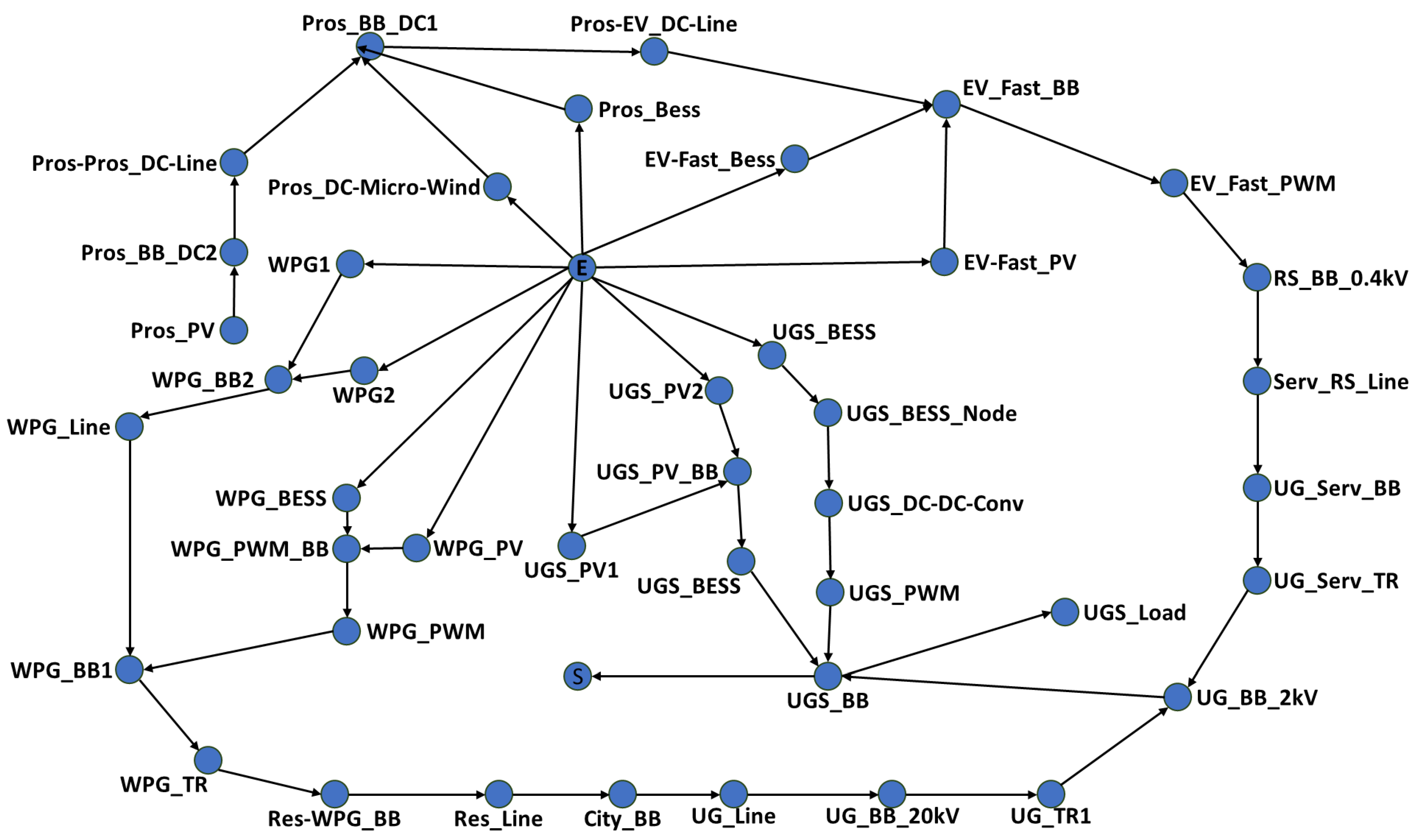
• Load feeding reliability evaluation for each grid consumption unit;
• Grid systemic reliability indices (SAIDI; SAIFI; etc).

The attention is preliminarily focused on the underground area which represents a small section of a metro network and an urban surface metro circuit of a small city.

It is constituted by the AC 20 kV busbar which is connected to the 2 kV bus (UG_BB_2 kV) by UG_TR1 and UG_TR2 power transformers. The Underground (UG_Load) and the Surface Underground (UGS_Load) loads are DC consumption units, while UG_Serv_AC-Load1 and UG_Serv_AC-Load2 are the AC ones.

DC consumption units are connected to the relative bus by power electronics converters, UG_BB_2 kV busbar is connected to UGS_BB bus by a DC/AC converter, while the AC loads are interfaced by a transformer (UG_Serv_TR).

The proposed methodology has been applied to each of these systems, converters, to the transformer and overhead distribution lines.

As an example, once the input data have been acquired (time series, manufacturer data, mission time), the reliability of the overhead distribution line connecting the UG_Serv_AC-Load1 to the UG_Serv_BB bus is calculated considering a 50,000 h mission time t.

Table 3. Proposed method application to an overhead distribution line.

Component	t [h]	αline [h]	βline	λwear_out [h−1]	πS_line	πE_line	πQ-line	λline [h−1]
Overhead Line	50,000	438,000	2	5.21 × 10−7	0.25	5	2.5	4.04 × 10−6

reports the details of the calculated values. In particular, λ_{wear_out} is determined considering α_line equal to 438,000 h and β_line equal to 2.

The evaluation of the line temperature in the different operating conditions indicated by the time series highlights the presence of two thermal cycles per day. The thermal stress factor π_{S_line} is calculated analyzing the line thermal cycles with relative minimum and maximum operative temperatures. Its value is reported in Table 3 with the π_{E_line} and π_Q-line user-defined ones. Finally, a line failure rate λ_line of 4.04 × 10⁻⁶ failure per hours is obtained by Equation (8) formula.

Applying the proposed methodology to the underground components, the failure rates and MTBFs values reported in

Table 4. Results of the underground area reliability assessment.

Component	Failure Rate [h−1]	MTBF [h]	MTBF [yr]
Overhead Lines	(4–6) × 10−6	250,000–166,666	28.53–19
Power Transformer UG_SERV_TR	6.41 × 10−6	155,946	17.80
DC/DC Converter UGS_BESS_DC-DC-Conv	7.08 × 10−6	141,249	16.12
DC/DC Converter UGS_PV_DC-DC-Conv	9.30 × 10−6	107,505	12.27
DC/AC Converter UGS_PWM	17.5 × 10−6	57,289	6.54
DC/AC Converter UG_PWM	7.03 × 10−6	142,245	16.24
PV Plant UGS_PV1	12.1 × 10−6	82,783	9.45
PV Plant UGS_PV2	12.1 × 10−6	82,783	9.45

are carried out.

In detail, overhead lines are continuously exposed to atmospheric and wear-out conditions. According to the analysis carried out, they are affected by a failure rate in the range of (4–6)∙failures per million hours. The specific values depend on circulating currents and thermal cycles of each line.

Referring to the power transformer “UG_SERV_TR”, its reliability assessment is conducted for an installation in an uncontrolled environment. As reported in the single-line diagram (Figure 10), UGS_BESS_DC-DC-Conv and UGS_PV_DC-DC-Conv converters interface the PV plants (UGS_PV1 and UGS_PV2) and the storage system (UGS_BESS) to the underground DC bus. UGS_PWM is the bidirectional inverter installed to source and sink operations to/from the MV AC bus. As reported in Table 4, the UGS_BESS_DC-DC-Conv and UGS_PV_DC-DC-Conv are characterized by MTBF values of 141249 and 107505 h, respectively, corresponding to about 16 and 12 years. UGS_PWM and UG_PWM inverters present 57289 and 142245 h MTBFs, respectively. Different reliability performance levels for these inverters are mainly due to the different environmental conditions where such systems are installed.

The reliability indicators for PV plants (UGS_PV1 and UGS_PV2) are calculated considering PV modules equipped with Distributed Maximum Power Point Tracking (DMPPT) converters [26] which control the PV source to continuously match the Maximum Power Point (MPP) conditions.

Furthermore, systemic reliability indices [29] are calculated for the power system under investigation reported in

Table 5. Systemic reliability indices.

Index	Value
ASAI [–]	0.99998
CAIDI [h]	10
CAIFI [1/c yr]	0.03533
ENS [kWh/yr]	0.07671
SAIDI [h/c yr]	0.17666
SAIFI [1/c yr]	0.01767

h = hours; c = customers; yr = yearly.

.

According to SAIFI and SAIDI values, each customer of the considered urban hybrid grid averagely experiences 11 min of outages in a year. The obtained ASAI indicates the service is available in 99.99% of the hours in which the customer demands it. CAIFI and CAIDI values underline a very low mean frequency of sustained interruptions for those customers experiencing sustained interruptions and that the mean time of 10 h is necessary to restore the service. ENS indicates that the total amount of energy not delivered to the system loads over a yearly time horizon is, on average, 0.07671 kWh.

The conducted systemic indicators evaluate the entire grid performance, but they do not provide quantitative data about the supply service reliability of the present consumption units.

Furthermore, the defined “load feeding reliability” index is calculated for each consumption unit of the considered grid. Relative values are graphically reported in Figure 13 by arrow symbols. They are colored according to the graphic scale (depicted in the same figure) from the most reliably supplied to the least reliably supplied loads. The “load feeding reliability” indicator provide significant information for grid operators (TSOs, DSOs) and prosumers/users. Referring to the underground (UG_Load), to the surface (UGS_Load) and to services (UG_Serv_AC-Load1, UG_Serv_AC-Load2) consumption units, the calculated “load feeding reliability” indices are 0.443, 0.969, 0.593 and 0.593, respectively. These results highlight the necessary improvement in the underground transportation units and service load supply. Surface transportation units are, instead, characterized by reliable sourcing paths.

The calculation of load feeding reliability and the identification of reliability criticalities in grids and microgrids represent meaningful outcomes since they could contribute to design, optimize and control the power system devices to avoid overstressing conditions.

Mesh and ring sections of the grid can assure higher sourcing reliability for their loads than the radial ones since different feeding paths can be activated (Figure 13). In Figure 14, it is noted that the User_AC-Load (clear orange arrowed unit) is connected in a radial portion of the grid. It presents a lower (0.559) load feeding reliability index than the Pros_AC-Load one (0.664) connected to a ring section of the considered power system, thus highlighting that multiple feeding paths assure a more reliable feeding capacity to the load points.

Different load systems are characterized by the same load feeding reliability if they are connected to the same bus and they are subjected to the same quality levels and environmental conditions, as reported by orange and yellow arrows.

5. Conclusions

Power systems are characterized by electrical, electronic, electromechanical and electrochemical components which have to assure reliable functioning mode. The need for a general RPM, customizable for grid components of different typologies, motivated the conducted study. Thermal (π_S), environmental (π_E) and quality stressing (π_Q) factors, which affect grid component behavior, are considered. In addition, the Weibull parameters of the system are considered for modeling component ageing phenomena.

The reliability assessment is completed with key indicator calculations (ASAI, CAIDI, CAIFI, ENS, SAIDI and SAIFI) for an underground transportation area.

The results from this work underline the following:

(i) 

The developed RPM can be applied to power transformers, overhead lines, interfacing power converters (DC/AC and AC/DC ones) and renewable plants;

(ii) 

Introduced operative environment and stressing agents (salt, solar radiation, etc.) permit us to accurately take into account actual factors impacting on each component/system.

(iii) 

The “load feeding reliability” index, calculated for each consuming unit of the power system under investigation, provides meaningful information in terms of unreliable supply paths. The identification of this issue can support TSO, DSO and prosumers to improve generation path reliability (for instance, adopting redundant solutions to avoid supply interruption).

Future research will take advantage of the proposed method to evaluate components reliability impact on power systems adequacy. In addition, the proposed methodology will be integrated in an advanced tool for grid adequacy, resilience and security calculation.

References

1. Porsinger, T.; Janik, P.; Leonowicz, Z.; Gono, R. Modelling and Optimization in Microgrids. Energies 2017, 10, 523. [Google Scholar] [CrossRef]
2. Yang, Z.; Han, J.; Wang, C.; Li, L.; Li, M.; Yang, F.; Lei, Y.; Hu, W.; Min, H.; Liu, Y. Emergency Power Supply Restoration Strategy for Distribution Network Considering Support of Microgrids with High-Dimensional Dynamic Correlations. Electronics 2023, 12, 3246. [Google Scholar] [CrossRef]
3. USA Department of Defense. MIL-HDBK-217F—Military Handbook—Reliability Prediction of Electronic Equipment; USA Department of Defense: Washington, DC, USA, 1990; ISBN 9150200801.
4. Reliability Analysis Center. PRISM & Failure Mode/Mechanical Distribution Document; Reliability Analysis Center: Rome, NY, USA, 1997. [Google Scholar]
5. FIDES Group. FIDES Guide 2022—Reliability Methodology for Electronic Systems; FIDES Group: Accra, Ghana, 2022. [Google Scholar]
6. Pougnet, P.; Bayle, F.; Maanane, H.; Dahoo, P.R. Reliability Prediction of Embedded Electronic Systems: The FIDES Guide. In Embedded Mechatronic Systems; Elsevier: Amsterdam, The Netherlands, 2019; pp. 189–216. [Google Scholar]
7. Charruau, S.; Guerin, F.; Dominguez, J.H.; Berthon, J. Reliability Estimation of Aeronautic Component by Accelerated Tests. Microelectron. Reliab. 2006, 46, 1451–1457. [Google Scholar] [CrossRef]
8. Real, D.; Calvo, D.; Musico, P.; Jansweijer, P.; Colonges, S.; van Beveren, V.; Carriò, F.; Pellegrini, G.; Díaz, A.F. Reliability Studies for the White Rabbit Switch in KM3NeT: FIDES and Highly Accelerated Life Tests. J. Instrum. 2020, 15, C02042. [Google Scholar] [CrossRef]
9. Yakymets, N.; Adedjouma, M. Model-Based Quantitative Fault Tree Analysis Based on FIDES Reliability Prediction. In Proceedings of the 2020 IEEE International Symposium on Software Reliability Engineering Workshops (ISSREW), Coimbra, Portugal, 12–15 October 2020; IEEE: New York, NY, USA, 2020; pp. 161–162. [Google Scholar]
10. Bourbouse, S.; Giraudeau, M.; Briard, H. Adapting FIDES for Reliability Predictions Aimed at Space Applications. In Proceedings of the 2019 Annual Reliability and Maintainability Symposium (RAMS), Orlando, FL, USA, 28–31 January 2019; IEEE: New York, NY, USA, 2019; pp. 1–6. [Google Scholar]
11. Prodanov, P.I.; Dankov, D.D.; Madzharov, N.D. Research of Reliability of Power Thyristors Using Methods MIL-HDBK-217F and FIDES. In Proceedings of the 2020 21st International Symposium on Electrical Apparatus & Technologies (SIELA), Bourgas, Bulgaria, 3–6 June 2020; IEEE: New York, NY, USA, 2020; pp. 1–4. [Google Scholar]
12. Held, M.; Fritz, K. Comparison and Evaluation of Newest Failure Rate Prediction Models: FIDES and RIAC 217Plus. Microelectron. Reliab. 2009, 49, 967–971. [Google Scholar] [CrossRef]
13. Pandian, G.P.; Das, D.; Li, C.; Zio, E.; Pecht, M. A Critique of Reliability Prediction Techniques for Avionics Applications. Chin. J. Aeronaut. 2018, 31, 10–20. [Google Scholar] [CrossRef]
14. Vasquez, W.A.; Jayaweera, D.; Jativa-Ibarra, J. Advanced Aging Failure Model for Overhead Conductors. In Proceedings of the 2017 IEEE PES Innovative Smart Grid Technologies Conference Europe (ISGT-Europe), Torino, Italy, 26–29 September 2017; IEEE: New York, NY, USA, 2017; pp. 1–6. [Google Scholar]
15. Singh, J.; Sood, Y.R.; Verma, P. The Influence of Service Aging on Transformer Insulating Oil Parameters. IEEE Trans. Dielectr. Electr. Insul. 2012, 19, 421–426. [Google Scholar] [CrossRef]
16. Peyghami, S.; Wang, Z.; Blaabjerg, F. A Guideline for Reliability Prediction in Power Electronic Converters. IEEE Trans. Power Electron. 2020, 35, 10958–10968. [Google Scholar] [CrossRef]
17. Awadallah, S.K.E.; Milanovic, J.V.; Jarman, P.N. The Influence of Modeling Transformer Age Related Failures on System Reliability. IEEE Trans. Power Syst. 2015, 30, 970–979. [Google Scholar] [CrossRef]
18. Adinolfi, G.; Ciavarella, R.; Graditi, G.; Ricca, A.; Valenti, M. A Planning Tool for Reliability Assessment of Overhead Distribution Lines in Hybrid AC/DC Grids. Sustainability 2021, 13, 6099. [Google Scholar] [CrossRef]
19. Petrarca, C. II Trasformatore. In Appunti del Corso di Elettrotecnica; Università Federico II: Naples, Italy, 2021. [Google Scholar]
20. Mirzai, M.; Gholami, A.; Aminifar, F. Failures Analysis and Reliability Calculation for Power Transformers. J. Electr. Syst. 2006, 2, 1–12. [Google Scholar]
21. Pei, X.; Cwikowski, O.; Vilchis-Rodriguez, D.S.; Barnes, M.; Smith, A.C.; Shuttleworth, R. A Review of Technologies for MVDC Circuit Breakers. In Proceedings of the IECON 2016—42nd Annual Conference of the IEEE Industrial Electronics Society, Florence, Italy, 24–27 October 2016; IEEE: New York, NY, USA, 2016; pp. 3799–3805. [Google Scholar]
22. Meyer, C.; Schroder, S.; DeDoncker, R.W. Solid-State Circuit Breakers and Current Limiters for Medium-Voltage Systems Having Distributed Power Systems. IEEE Trans. Power Electron. 2004, 19, 1333–1340. [Google Scholar] [CrossRef]
23. Erickson, R.W.; Maksimovic, D. Fundamentals of Power Electronics; Springer: New York, NY, USA, 2001; ISBN 9780792372707. [Google Scholar]
24. Cardoso, A.J.M.; Bento, F. Diagnostics and Fault Tolerance in DC–DC Converters and Related Industrial Electronics Technologies. Electronics 2023, 12, 2341. [Google Scholar] [CrossRef]
25. Li, Z.; Wang, Y.; Shi, L.; Huang, J.; Cui, Y.; Lei, W. Generalized Averaging Modeling and Control Strategy for Three-Phase Dual-Active-Bridge DC-DC Converters with Three Control Variables. In Proceedings of the 2017 IEEE Applied Power Electronics Conference and Exposition (APEC), Tampa, FL, USA, 26–30 March 2017; IEEE: New York, NY, USA, 2017; pp. 1078–1084. [Google Scholar]
26. Merenda, M.; Iero, D.; Pangallo, G.; Falduto, P.; Adinolfi, G.; Merola, A.; Graditi, G.; Della Corte, F. Open-Source Hardware Platforms for Smart Converters with Cloud Connectivity. Electronics 2019, 8, 367. [Google Scholar] [CrossRef]
27. Graditi, G.; Adinolfi, G. Temperature Influence on Photovoltaic Power Optimizer Components Reliability. In Proceedings of the International Symposium on Power Electronics Power Electronics, Electrical Drives, Automation and Motion, Sorrento, Italy, 20–22 June 2012; IEEE: New York, NY, USA, 2012; pp. 1113–1118. [Google Scholar]
28. Sayed, A.; El-Shimy, M.; El-Metwally, M.; Elshahed, M. Reliability, Availability and Maintainability Analysis for Grid-Connected Solar Photovoltaic Systems. Energies 2019, 12, 1213. [Google Scholar] [CrossRef]
29. Parol, M.; Wasilewski, J.; Wojtowicz, T.; Arendarski, B.; Komarnicki, P. Reliability Analysis of MV Electric Distribution Networks Including Distributed Generation and ICT Infrastructure. Energies 2022, 15, 5311. [Google Scholar] [CrossRef]
Figure 1. Reliability modeling for a grid component.
Electronics 13 00275 g001
Figure 2. Lumped parameter equivalent circuits of an MV line.
Electronics 13 00275 g002
Figure 3. Lumped parameter equivalent circuits of an MV short line.
Electronics 13 00275 g003
Figure 4. Reliability evaluation process for a line overtemperature calculation.
Electronics 13 00275 g004
Figure 5. Ideal transformer equivalent circuit: simplified model [19].
Electronics 13 00275 g005
Figure 6. Transformer equivalent circuit [19].
Electronics 13 00275 g006
Figure 7. DAB converter circuit.
Electronics 13 00275 g007
Figure 9. Benchmark grid used for reliability assessment.
Electronics 13 00275 g009
Figure 10. Underground area and road service area.
Electronics 13 00275 g010
Figure 11. Residential and wind area.
Electronics 13 00275 g011
Figure 12. Graph of possible supply paths relative to UGS_Load.
Electronics 13 00275 g012
Figure 13. Map of load feeding reliability for considered grid loads.
Electronics 13 00275 g013
Figure 14. Load feeding reliability for loads in radial and ring grids.
Electronics 13 00275 g014