Article

Camera–LiDAR Calibration Using Iterative Random Sampling and Intersection Line-Based Quality Evaluation

1
Department of Intelligent Mechatronics Engineering, Sejong University, Seoul 05006, Republic of Korea
2
Department of Electronic Engineering, Korea National University of Transportation, Chungju 27469, Republic of Korea
*
Author to whom correspondence should be addressed.
Electronics 2024, 13(2), 249; https://doi.org/10.3390/electronics13020249
Submission received: 29 November 2023 / Revised: 23 December 2023 / Accepted: 1 January 2024 / Published: 5 January 2024

Abstract

:
This paper proposes a novel camera–LiDAR calibration method that utilizes an iterative random sampling and intersection line-based quality evaluation using a foldable plane pair. Firstly, this paper suggests using a calibration object consisting of two small planes with ChArUco patterns, which is easy to make and convenient to carry. Secondly, the proposed method adopts an iterative random sampling to make the calibration procedure robust against sensor data noise and incorrect object recognition. Lastly, this paper proposes a novel quality evaluation method based on the dissimilarity between two intersection lines of the plane pairs from the two sensors. Thus, the proposed method repeats random sampling of sensor data, extrinsic parameter estimation, and quality evaluation of the estimation result in order to determine the most appropriate calibration result. Furthermore, this method can also be used for the LiDAR–LiDAR calibration with a slight modification. In experiments, the proposed method was quantitively evaluated using simulation data and qualitatively assessed using real-world data. The experimental results show that the proposed method can successfully perform both camera–LiDAR and LiDAR–LiDAR calibrations while outperforming the previous approaches.

1. Introduction

Recent increases in societal demand for autonomous vehicles and mobile robots have led to active research in using various sensors to perceive their surroundings automatically [1,2,3]. Specifically, research focusing on the fusion of multiple heterogeneous sensors is gaining attention to ensure stable performance [4,5]. A representative example of sensor fusion used for environmental perception uses a camera and Light Detection And Ranging (LiDAR) together. Cameras can provide detailed appearance and color information of objects but require additional sophisticated algorithms to extract 3D information. On the other hand, LiDAR has the advantage of directly providing precise 3D information of objects but does not provide detailed appearance and color information. Therefore, by combining a camera and LiDAR, detailed shape, color, and 3D information of surrounding objects can be simultaneously acquired to improve recognition performance [6,7].
To effectively integrate and use cameras and LiDARs, it is essential to conduct extrinsic calibration, which estimates the geometric relationship between sensors installed at different positions and facing different directions. Various methods have been proposed for extrinsic calibration. However, most of the previous methods have the limitation of being vulnerable to noise occurring in sensor data or calibration object recognition. Thus, calibration errors occur when sensor data are incorrectly acquired or calibration objects are poorly recognized. Previous methods mostly solve these problems by manually removing noisy data or poor recognition results [8,9,10,11,12,13,14,15,16]. However, this manual approach has a critical limitation that prevents the calibration process from being fully automatic. To overcome this limitation, this paper proposes a method in which the calibration process is performed entirely automatically and is robust to errors in sensor data or calibration object recognition results. To this end, this paper proposes a method that iteratively conducts a random selection of sensor data, calibration of extrinsic parameters, and evaluation of the calibration result. In particular, the proposed method uses a novel evaluation criterion based on the dissimilarity of 3D lines to select the most appropriate calibration result. Additionally, previous methods have the limitation that the shape of the calibration object is challenging to manufacture [16,17,18,19,20,21,22,23]. To mitigate this limitation, this paper proposes a simple calibration object that is easy to make and convenient to carry because it consists of two small planes with ChArUco (Checkerboard + ArUco) patterns on them. When using the proposed object, the quality of the calibration result can be evaluated based on the intersection lines of the two planes of the object. Besides the above advantages, the proposed method and object can be used not only for camera–LiDAR calibration but also for LiDAR–LiDAR calibration.
In detail, the proposed method is performed as follows. First, images and point clouds are acquired from the camera and LiDAR, respectively, while changing the poses of the calibration object. After that, 3D plane pairs are detected from the data of each sensor. In the case of the camera, corners are detected from images, intrinsic and extrinsic parameters of the camera are obtained, and 3D plane pairs are estimated by applying the least squares method to three-dimensionally reconstructed corners. In the case of the LiDAR, 3D plane pairs are estimated by applying Random Sample Consensus (RANSAC) to point clouds. Once 3D plane pairs are obtained from the two sensors, extrinsic parameters (rotation and translation) that match the plane pairs of the camera and LiDAR are iteratively estimated by randomly selecting 3D plane pairs. The extrinsic parameters are first estimated by the least squares method and then refined by the nonlinear optimization. Iteratively estimated extrinsic parameters are evaluated based on the dissimilarity between 3D intersection lines of the plane pairs from the camera and LiDAR. Finally, the one that provides the smallest dissimilarity is selected as the most appropriate calibration result. In the experiments, the proposed method was quantitatively evaluated using simulation data and quantitatively evaluated using real-world data. The experimental results show that the proposed method accurately determines the extrinsic parameters of two sensors and outperforms previous approaches.
The rest of this paper is organized as follows. Section 2 describes related research. Section 3 introduces the suggested calibration object and describes the proposed calibration method in detail, and Section 4 presents experimental results and discussion. Finally, this paper is concluded with a summary in Section 5.

2. Related Works

Extrinsic calibration is the task of estimating the rigid body transformations between multiple sensors. According to the need for target objects (calibration objects), extrinsic calibration methods can be divided into target-based and targetless. Since this paper focuses on proposing a target-based method, this literature review will only introduce target-based methods. Target-based methods have been widely used because they provide reliable calibration results, and various target objects have been suggested. These target-based methods can be categorized into the 2D object-based approach and 3D object-based approach.

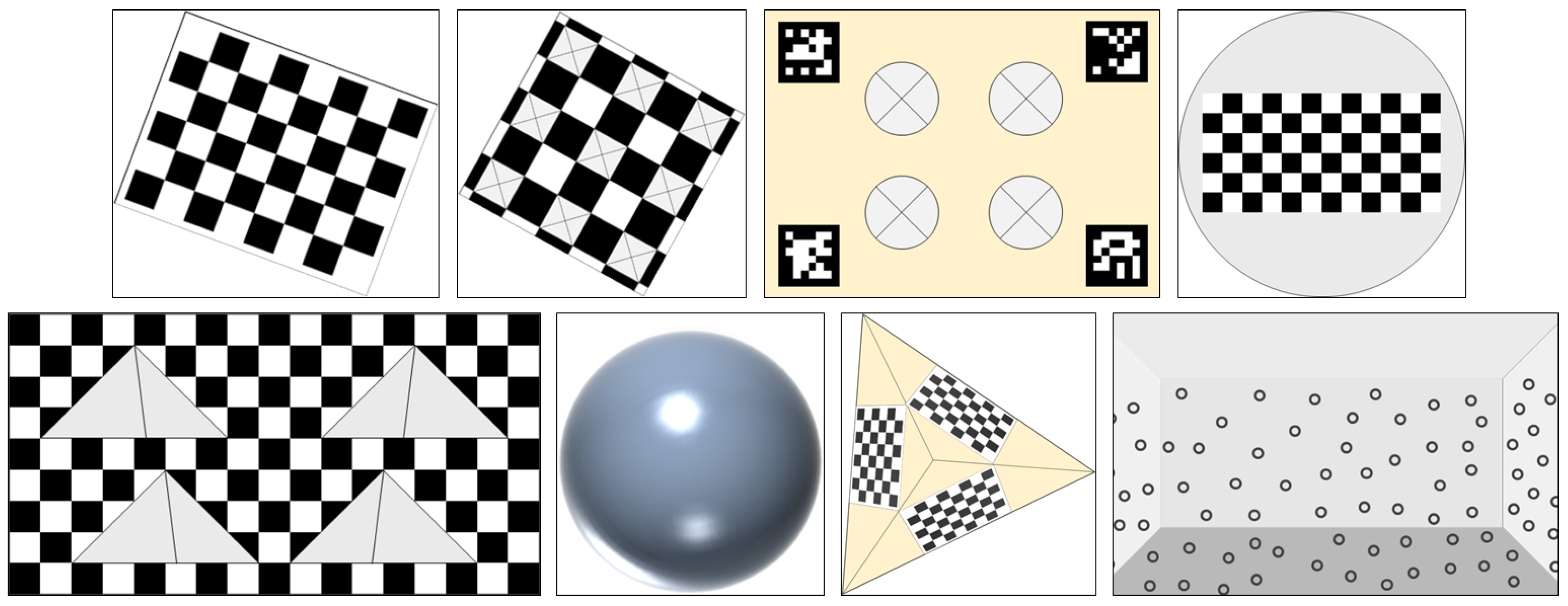
2.1. Two-Dimensional Object-Based Approach

Most 2D object-based methods use a checkerboard, rectangular plane, or plane with holes for the camera–LiDAR extrinsic calibration. The top row of Figure 1 shows examples of 2D objects used in previous methods. Zhang et al. [8] proposed a method that calibrates a 2D LiDAR and camera using a checkerboard. This method estimated extrinsic parameters based on the planar constraint using the least squares method followed by nonlinear optimization based on point-to-plane distance. Unnikrishnan et al. [9] suggested a calibration method similar to [1], but this method deals with a 3D LiDAR rather than a 2D LiDAR. Rodriguez et al. [10] utilized a plane with a single circular hole. This method finds the center of the circular hole from two sensors, and it estimates extrinsic parameters using the least squares method with the point correspondences followed by nonlinear optimization based on Euclidean distance between corresponding centers. Geiger et al. [11] proposed a method that utilizes multiple checkerboards. This method finds checkerboard planes in point clouds and images, and it estimates extrinsic parameters by aligning normal vectors of checkerboard planes and minimizing point-to-plane distance. Kim et al. [12] suggested a similar approach to [11]. The major difference from [11] is that this method estimates translation between two sensors by minimizing the distance between two planes: one from the camera and the other from the LiDAR. Sui et al. [13] proposed a calibration method based on a plane with four circular holes. This method finds circles in point clouds and images and roughly estimates extrinsic parameters based on the centers and radiuses of detected circles. It then refines them by minimizing distances between depth discontinuities of point clouds and edge pixels of images. Zhou et al. [14] suggested a calibration method based on four checkerboard edges. This method estimates the extrinsic parameters through the geometric correspondence between four edges of the plane in point clouds and planar parameters in images, and it optimizes them by minimizing point-to-plane and point-to-line distances. Tu et al. [15] utilized a planar checkerboard for finding 2D–3D point correspondences. This method extracts 2D corners of the checkerboard in images and corresponding 3D points in point clouds by finding the checkerboard vertexes. It estimates extrinsic parameters using the efficient Perspective-n-Points (PnP) and minimizing the reprojection errors. Xie et al. [16] proposed a method that uses a checkerboard with square holes, as shown in Figure 1 (top second image). This method extracts corresponding points in two sensors, and it calculates a linear alignment matrix as extrinsic parameters by minimizing the distance between 2D points in images and projected 3D points. Huang et al. [24] suggested a method based on a 2D diamond-shaped plane with a visual marker. This method extracts corresponding plane vertices in images and point clouds, and it estimates extrinsic parameters using the standard PnP and intersection over union (IoU)-based optimization. Mishra et al. [25] utilized a marker-less planar target. This method finds edges and corners in images and boundary points in point clouds, and it estimates extrinsic parameters using a nonlinear least squares method based on point-to-plane and point-to-back-projected plane constraints. Xu et al. [26] proposed a triangular board-based calibration method. This method extracts a 3D plane and edges of the triangular board to obtain its 3D vertex locations. Extrinsic parameters are estimated based on the 3D vertexes in point clouds and 2D corners in images after removing 3D vertexes whose angles differ from their actual values. Beltrán et al. [17] used a plane with four circular holes as well as four ArUco markers, as shown in Figure 1 (top third image). This method detects the centers of four holes in point clouds and finds planar parameters and the centers of four holes in images. It estimates extrinsic parameters based on point-to-point distance using the least squares method. Li et al. [18] suggested a method based on a checkerboard with four circular holes. In this method, the centers of the holes are designed to be the same as the centers of the checkerboard rectangles. It finds the centers of the holes in point clouds and the centers of the rectangles in images. Extrinsic parameters are estimated by minimizing the projected distance. Liu et al. [19] utilized a circular plane with a checkerboard printed on it, as shown in Figure 1 (top right image). This method finds the circle centers and the plane normal vectors in both point clouds and images. It estimates extrinsic parameters based on these correspondences using the standard PnP and nonlinear optimization with the reprojection error. Yan et al. [20] proposed a method that uses a checkerboard plane with four circular holes similar to [18]. This method detects the centers of the four holes in point clouds based on depth discontinuities and those in images based on the calibration board size. It estimates the extrinsic parameters by minimizing the reprojection error of the hole centers.

2.2. Three-Dimensional Object-Based Approach

Most 3D object-based methods perform extrinsic calibration using polyhedrons or spheres. This approach has been less actively researched than the 2D object-based approach due to the difficulties in making calibration objects. The bottom row of Figure 1 shows examples of 3D objects used in previous methods. Gong et al. [28] proposed a method that uses an arbitrary trihedron. This method estimates planes of the trihedron in point clouds using 3D information and those in images using the planarity constraint established between two frames. It estimates extrinsic parameters using the least squares method followed by nonlinear optimization based on the relation between corresponding planes. Pusztai and Hajder [29] suggested a method based on a cuboid with a known size. This method estimates three perpendicular planes of the cuboid and calculates its corners in point clouds. It also finds the corresponding corners in images using the Harris corner detector. Extrinsic parameters are estimated by applying the Effective-PnP to the corresponding points. Cai et al. [21] utilized a calibration object composed of a checkerboard and four triangular pyramid shapes on it, as shown in Figure 1 (bottom left image). This method finds vertexes of the triangular pyramids in point clouds and corresponding points in images by detecting corners of the checkerboard. It calculates the transformation between 3D vertexes and 2D corners and estimates extrinsic parameters based on the transformation. Kümmerle et al. [30] proposed a spherical object-based method. This method finds sphere centers by fitting 3D spheres in point clouds and calculates the corresponding sphere centers in images by fitting ellipses based on edge pixels. Extrinsic parameters are estimated by finding the rigid transformation that minimizes the sum of squared point-to-ray distances. Tóth et al. [27] suggested a similar method to [30] based on a spherical object. This method estimates extrinsic parameters by calculating the rigid transformation between the corresponding sphere centers based on the least squares method. Erke et al. [31] utilized three orthogonal planes with a checkerboard printed on one of them. This method finds extrinsic parameters by separately conducting LiDAR–robot and camera–robot calibrations. The former is based on normal vectors of three orthogonal planes, and the latter is based on the checkerboard on one of the planes. Bu et al. [22] proposed using a triangular pyramid with three checkerboard patterns on its three planes, as shown in Figure 1 (bottom third image). This method estimates the LiDAR’s extrinsic parameters based on the fitting result of the three planes and the camera’s extrinsic parameters based on the detection result of the three checkerboards. It combines these parameters to obtain the initial extrinsic parameters between two sensors and finds the optimal parameters by minimizing the point-to-plane distance. Fang et al. [23] suggested a method based on a panoramic infrastructure built by covering a room with circular markers, as shown in Figure 1 (bottom right image). This method reconstructs the 3D structures of the infrastructure using a stereo camera before the calibration. During the calibration, it localizes the LiDAR based on lines and corners and localizes the camera based on the PnP using marker centers. Extrinsic parameters are estimated based on the localization results of two sensors. Agrawal et al. [32] utilized a triangular pyramid of silver reflecting foil on a rectangular plane with a red boundary. This method finds the triangular centers by clustering the points with high reflectivity in point clouds and corresponding centers in images using a deep-learning-based object detector. It estimates extrinsic parameters by applying the PnP to these 2D–3D correspondences.
Table 1 shows that the previous methods are classified according to the calibration object, the creation difficulty of the calibration object, and the calibration quality evaluation method. In addition, this table shows that the proposed method utilizes an easily producible calibration object compared to the previous methods and includes a method for evaluating calibration results.

3. Proposed Method

3.1. Proposed Calibration Object

In this paper, we propose a calibration object consisting of two small-sized planes, designed in this way to be easy to manufacture, convenient to carry, and automatically perform object recognition. Figure 2 shows the proposed calibration object. The size of the two planes that make up this object are each 50 × 50 cm, and the object was made to be foldable for convenient portability. The two planes are composed of a ChArUco board [33] to make it easy to automatically recognize the corner positions and indices. ChArUco is an integrated marker that combines a checkerboard with an ArUco marker. By detecting the corner of the checkerboard and recognizing the ArUco marker around the detected corner, location and index information can be obtained simultaneously. At this time, in order to facilitate automatic distinction between the two planes, ChArUco markers of different sizes are printed on the two planes. The proposed calibration object uses 6 × 6 ArUco markers on the left plane and 5 × 5 ArUco markers on the right plane to distinguish between two planes automatically. Once images and point clouds are obtained from the two sensors while changing the position and orientation of the calibration object, LiDAR–camera calibration is performed by detecting 3D plane pairs. During the calibration, the proposed method uses the intersection of the two planes (green line in Figure 2) to select the most appropriate calibration result. Detailed information is provided starting from Section 3.2.

3.2. Overview of the Proposed Method

The overall structure of the proposed method is presented in Figure 3. First, the proposed method uses the camera’s images and LiDAR’s point clouds acquired by changing the calibration object in Figure 2 to different positions and postures as inputs. At this time, the calibration object must be located where the field-of-view (FOV) of the two sensors overlap. After acquiring data from the two sensors, two planes constituting the calibration object are estimated from the image and point cloud. This process is called two-plane estimation, and the two planes estimated from the image and the two planes estimated from the point cloud are called a two-plane pair (TPP). Several TPPs are obtained from the data acquired by changing the position and direction of the calibration object, and a group of these TPPs is called a TPP set. The extrinsic parameter estimation method takes the TPP set as input and estimates the rotation and translation, which are external relationships between two sensors. The proposed method can also be used for LiDAR–LiDAR extrinsic calibration by only changing the two-plane estimation for the camera into the two-plane estimation for the LiDAR in Figure 3.
Figure 4 shows the flowchart of the extrinsic parameter estimation step in Figure 3. When the TPP set is input, some TPPs are randomly selected for the TPP set in the next step. The i-th randomly selected TPP subset is indicated as TPPisub, and the rotation and translation estimated from TPPisub are indicated as Ri and ti, respectively. The rotation and translation estimation consists of the least squares method based on the coincidence of planes and nonlinear optimization that minimizes point-to-plane distances. Once Ri and ti are estimated, their quality is evaluated based on the Intersection Line Difference (ILD) after aligning the coordinate systems of the two sensors. ILD is calculated based on the angle and distance differences between the intersection line of the two planes estimated from the image and the intersection line of the two planes estimated from the point cloud. The ILD is calculated from all TPPs included in the TPP set, and the mean ILD (mILD) is obtained by taking the average of the top 80%. The proposed method repeats the above process for a predetermined number and selects the rotation and translation that yield the smallest mILD as the final result. The number of TPP subsets used in the proposed method was 5, and the max iteration was set to 700. Details on these steps will be introduced in the following sections.

3.3. Three-Dimensional Plane Estimation

3.3.1. Camera-Based 3D Plane Estimation

The proposed method estimates the two planes of the calibration object three-dimensionally from images acquired by the camera. This process consists of three steps: corner detection, camera calibration, and 3D plane estimation. First, the corners of the ChArUco board squares are detected, and then the ArUco patterns are recognized to identify the corner IDs. OpenCV is used to perform ChArUco board creation, corner detection, and identification [34]. Figure 5a shows an example result of the corner detection and identification. Red and blue dots indicate the corner locations on the left and right planes, respectively, and the yellow numbers indicate the corner IDs. After that, camera calibration is performed based on the corner detection results. The camera calibration is conducted by Zang’s method [35], which is a representative method that estimates the intrinsic and extrinsic parameters of the camera based on the corners of the checkerboard taken from various angles. Finally, the 3D locations of the corners are calculated, and the 3D planes are estimated based on them. The 3D locations of the ChArUco board corners are calculated by Equation (1) using the rotation ( R C ) and translation ( t C ) between the ChArUco board coordinates and camera coordinates.
X c Y c Z c = R C X B Y B 0 + t C
where X c Y c Z c T and X B Y B 0 T are the 3D locations of the corner in the camera coordinates and ChArUco board coordinates, respectively. Because the ChArUco board is flat, the Z-axis value of X B Y B 0 T is zero. X B Y B 0 T can be determined from the predetermined geometry of the ChArUco board, and R C and t C are obtained through the camera calibration. In Figure 5b, red and blue dots show the reconstructed 3D corners of the left and right ChArUco boards, respectively. After that, the least squares method is applied to the 3D corners of each plane to estimate the parameters of the 3D plane. Figure 5c shows two 3D planes estimated by the 3D point in Figure 5b.

3.3.2. LiDAR-Based 3D Plane Estimation

As with the camera, the proposed method estimates the two planes of the calibration object three-dimensionally from point clouds acquired by the LiDAR. Unlike the camera, the LiDAR provides 3D location directly, so there is no need for a 3D location calculation. However, since the point cloud generally includes 3D points of objects other than the calibration object, as shown in Figure 6a, it is necessary to estimate the 3D planes robustly against these objects. For this purpose, this paper first selects the points within the region of interest (ROI) and then uses random sample consensus (RANSAC)-based 3D plane estimation [36]. Figure 6b shows an example result of the ROI-based point selection. This paper simply selects the points inside the predetermined area. If no other planar objects are around the LiDAR, the ROI is set based only on distance. In this case, the ROI is set to 2.0 m around the LiDAR. If other planar objects, such as walls, exist around the LIDAR, the ROI is set based on both distance and angle. The angular ROI is set using the rough angle at which the fields of view of the two sensors overlap. As shown in Figure 6b, the points after the ROI-based point selection still include objects other than the calibration object. Therefore, in this paper, 3D plane estimation is performed based on RANSAC, a representative estimator robust against outliers. To estimate two planes of the proposed calibration object, this paper first estimates one plane using RANSAC and removes all points close to the estimated plane. After that, RANSAC is used again for the remaining points to estimate the other plane. Figure 6c shows the 3D plane estimation result based on the point cloud in Figure 6b.

3.4. Extrinsic Parameter Estimation

3.4.1. Initialization and Optimization

Once the TPP (two-plane pair) set is obtained from the camera and LiDAR using the 3D plane estimation methods in Section 3.3, the proposed method randomly selects TPP subsets from the TPP set as described in the flowchart of Figure 4. This subsection explains how the proposed method estimates the extrinsic parameters of two sensors using the TPP subset. This process consists of two steps: parameter initialization and nonlinear optimization.
First, initial extrinsic parameters are estimated based on the relation between the corresponding 3D planes acquired by the two sensors. The corresponding 3D planes satisfy the relation in Equation (2).
n i C d i C = R 0 t T R 1 n i L d i L
where R and t indicate the rotation and translation between the camera and LiDAR. n i C T   d i C T and n i L T   d i L T are parameters of the corresponding i-th 3D planes estimated from the camera and LiDAR, respectively. n i C and n i L are 3 × 1 normal vectors of the two planes. d i C and d i L are scalar values that indicate distances between the two planes and the origin, respectively. When N pairs of planes are detected, R can be calculated by Equation (3) as a least-squares solution [11].
R = a r g m a x R i = 1 N n i C T R n i L = V U T i = 1 N n i L n i C T = U D V T
Once R is obtained, t can be calculated by Equation (4), which is derived from Equation (2).
d i C = t T R n i L + d i L t = p i n v L R T d L = ( n 1 L ) T ( n N L ) T ,         d = d 1 L d 1 C d N L d N C
where pinv indicates the pseudo inverse, L is a N × 3 matrix, and d is a N × 1 vector.
After estimating the initial R and t, nonlinear optimization is utilized to find R and t that minimize the point-to-plane distance (c) in Equation (5). To this end, Levenberg–Marquardt (LM), one of the representative nonlinear optimization methods, is used [37].
c = i = 1 N 1 M i L j = 1 M i L d i s t H x i , j L , π i C + 1 M i C k = 1 M i C d i s t H 1 x i , k C , π i L H = R t 0 T 1
where dist indicates the function for calculating the point-to-plane distance. H is a 4 × 4 matrix representing projective transformation that converts points in the LiDAR coordinates to the camera coordinates. x i , j L is the j-th point belonging to the i-th plane estimated from the LiDAR and x i , k C is the k-th point belonging to the i-th plane estimated from the camera. π i C and π i L are the parameters of the i-th plane estimated from the LiDAR and camera, respectively. M i L and M i C are the numbers of the 3D points in the i-th planes of the LiDAR and camera, respectively.

3.4.2. Quality Evaluation for Extrinsic Parameters

As shown in the flowchart of Figure 4, the proposed method repeats the process that randomly selects a TPP subset, estimates extrinsic parameters, and evaluates the quality of the estimation result. The extrinsic parameter estimation is described in the previous section, and this section explains the quality evaluation method for the estimated extrinsic parameters.
The proposed method evaluates the quality of extrinsic parameters based on the dissimilarity between the intersection lines of two planes. The suggested dissimilarity measure is called mean Intersection Line Difference (mILD), which is calculated as follows: First, the intersection line between the two planes of the proposed calibration object is calculated from the camera and LiDAR in the whole TPP set. After that, intersection lines in the camera coordinates are converted to the LiDAR coordinates based on the estimated extrinsic parameters. In Figure 7a,b, magenta and green lines are the intersection lines estimated from the camera and LiDAR, respectively. The left side of Figure 7c shows the result of overlapping Figure 7a,b. The Intersection Line Difference (ILD) is calculated based on the dissimilarity between the intersection line from the camera and that from the LiDAR, as shown on the right side of Figure 7c. In detail, the ILD consists of two types of difference: distance difference (ILD_distance) and angle difference (ILD_angle).
Figure 8 along with Equations (6) and (7) describe how ILD_distance and ILD_angle are calculated. In Figure 8, the magenta line ( l i n e c a m ) and green line ( l i n e l i d a r ) are the intersection lines from the camera and LiDAR, respectively. ILD_distance is calculated by Equation (6), which takes an average of d i . d i is a distance between a point ( p c a m i ) on l i n e c a m and the projected point of p c a m i onto l i n e l i d a r , as shown in Figure 8.
I L D _ d i s t a n c e = 1 n i = 1 n d i d i = v i × l l
In Figure 8 and Equation (6), c and l are direction vectors of l i n e c a m and l i n e l i d a r , respectively. p c a m i and p l i d a r i are randomly selected points on l i n e c a m and l i n e l i d a r , respectively. v i is a vector between p c a m i and p l i d a r i . n is the number of sample points and is set to 100 in this paper. ILD_angle is obtained by measuring the angle between the directional vectors of l i n e c a m and l i n e l i d a r as in Equation (7).
I L D _ a n g l e = cos 1 c · l c l
ILD (ILD_distance and ILD_angle) is calculated for all TPPs included in the TPP set. mILD (mILD_distance and mILD_angle) is calculated by averaging the smallest 80% of the ILDs in all TPPs. By excluding a certain percentage of ILDs with large values, mILD becomes more robust against situations where the sensor data or calibration object detection are erroneous. The ratio of TPPs included in the mILD calculation may change depending on the noise situation of the sensor or the performance of the object detection.
Finally, mILD is used to measure the quality of the estimated extrinsic parameters. In detail, as shown in the flowchart of Figure 4, the proposed method repeatedly estimated extrinsic parameters by randomly selecting TPP subsets, and it updates the extrinsic parameters only when they simultaneously reduce both mILD_distance and mILD_angle. Thus, this process selects the extrinsic parameters, which provide the smallest mILD as the final calibration result.

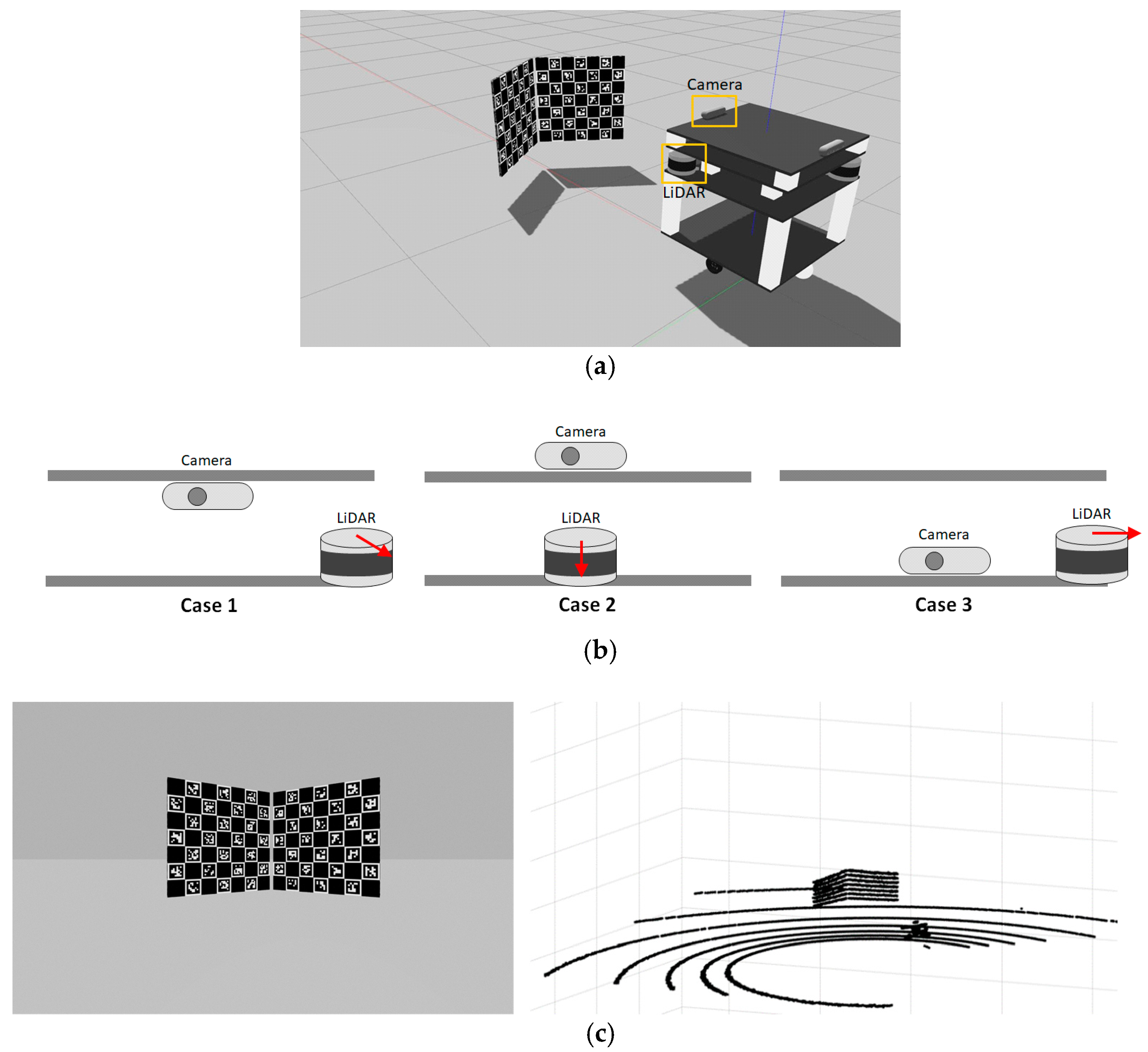
4. Experiment Results and Discussion

4.1. Simulation-Based Quantitative Evaluation

The proposed method was quantitatively evaluated based on a simulation using Gazebo [38]. In Figure 9, (a) shows the simulation environment, (b) indicates three different sensor configurations used in the simulation, and (c) presents example data acquired from two sensors. The same sensors as the actual sensors were used for the simulation: Intel RealSense D455 for the camera and Velodyne VLP-16 for the LiDAR. The camera and LiDAR noises were measured using the actual sensors and applied to the simulated sensor data: the standard deviation of the range noise was set to 0.0097 m for the LiDAR, and the peak signal-to-noise ratio (PSNR) of the image to 42 dB. The simulation was conducted with three different positions of the camera and LiDAR, as shown in Figure 9b. For each configuration, 20 images and point clouds were acquired while changing the poses of the calibration objects.
Table 2 shows a performance comparison of the proposed method with two other approaches. In this table, Method I estimates extrinsic parameters using all TPP sets based on the method described in Section 3.4.1. Most calibration methods use this type of approach based on the whole data. Method II uses the proposed sub-sampling method shown in the flowchart of Figure 4. However, this method evaluates the quality of the estimated parameters based on the point-to-plane distance instead of the proposed mILD. In other words, the parameters providing the smallest distance between the point and the plane are selected as the final result. In contrast, the proposed method performs the quality evaluation of the estimated parameters based on the proposed sub-sampling method, and the suggested mILD, as shown in Figure 4. This means that the parameters that provide the smallest mILD are selected as the final result. Table 2 includes the means and standard deviations of rotation and translation errors. These were calculated by applying the three methods 30 times to the simulation data with three sensor configurations. The error refers to the difference between the ground truth provided by the simulation and the result of the method. The rotation error is obtained by calculating the average of the angle errors of the three axes, and the translation error is also calculated in the same way.
In Table 2, the methods that use the proposed sub-sampling approach (Method II and Proposed method) perform significantly better than the method that does not use it (Method I). This is because the samples with erroneous data or incorrect plane estimation can negatively affect the estimation result when all samples are used. However, when using the proposed sub-sampling, these unfavorable samples are excluded during the random subset selection, which enables more precise estimation. Comparing the two methods using the suggested sub-sampling in Table 2, the proposed method evaluating parameters based on the proposed mILD outperforms Method II, which uses the point-to-plane distance-based quality evaluation. Upon closer examination of the errors between these two methods, it is evident that while the translation errors are quite similar, there is a relatively significant difference in the rotation errors. This difference can be attributed to the point-to-plane distance failing to adequately capture changes when rotation occurs in a direction perpendicular to the plane. In contrast, the proposed mILD considers not only the difference in translations (mILD_distance) but also the difference in orientations (mILD_angle), making it more robust to rotation compared to the point-to-plane distance. Therefore, through Table 2, it can be confirmed that the most precise calibration result is achieved when the proposed sub-sample method and mILD are used in conjunction.
Table 3 shows the performance comparison between the proposed method and the previous method in [14] implemented by [39], which is one of the widely used methods. The method in [14] uses a different type of calibration object (single rectangular checkerboard) from the proposed method. During the performance comparison, the three sensor configurations in Figure 9b were set to be the same, and only the calibration object was changed. Since the method in [14] performs calibration by detecting four sides of the checkerboard, this method has a strict condition that the data of the two sensors simultaneously contain all four sides of the checkerboard. Due to this, after acquiring the sensor data while changing the poses of the checkerboard, we manually selected some data satisfying the condition of the method in [14] for the performance comparison. This strict condition for the data acquisition makes the calibration process difficult, so it is a significant practical disadvantage of the method in [14].
In Table 3, the proposed method clearly outperforms the previous method in [14] in terms of both translation and rotation errors. There may be two main reasons for this result. One is that the method in [14] uses points located at the boundary of the checkerboard, which may not correspond to the actual boundary due to the low resolution of the LiDAR. Noise on these boundary points affects the performance of the line detection. The other is that the method does not include a process to filter out noisy sensor data or inaccurate detection results, unlike the proposed method.

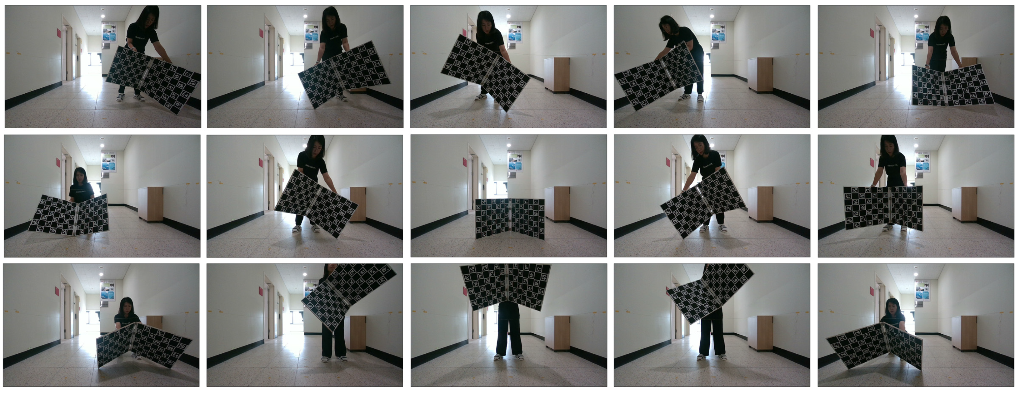
4.2. Real-Data-Based Qualitative Evaluation

In order to check whether the proposed method operates correctly in a real-world environment, we installed a camera and LiDAR on a robot-shaped jig and acquired sensor data from them to perform the calibration. In Figure 10, (a) shows the two sensors attached to the robot-shaped jig, and (b) presents example data acquired from the two sensors. In this experiment, the same sensors as those in the simulation were used: Intel RealSense D455 for the camera and Velodyne VLP-16 for the LiDAR. The calibration object was placed 1~2 m in front of the sensors, and 20 images and point clouds were acquired by changing its pose. Figure 11 shows example images acquired by the camera while changing the pose of the calibration object for the camera–LiDAR calibration.
Figure 12 shows the updating process of the extrinsic parameters based on the suggested mILD in real-world data. In this figure, (a–c) show consecutively resulting calibration results as the parameter estimation and quality evaluation in Figure 4 are repeated. Magenta and green lines indicate the intersection lines of the two planes from the camera and LiDAR, respectively. It can be clearly seen that the magenta and green lines become closer to each other as the iteration progresses. This means that the quality of the parameters is improving. It can also be noticed that the red points, the projected 3D points of the calibration object, are becoming more consistent with the image of the calibration object as the iteration progresses. Figure 13 shows the results of projecting the LiDAR’s point clouds onto the camera’s images using the final calibration result of the proposed method. Even when objects with different shapes are located at various distances, it can be confirmed that the point clouds of the LiDAR are correctly aligned with the images of the camera. This result shows the proposed method can successfully calibrate the camera and LiDAR in real-world situations.

4.3. LiDAR–LiDAR Calibration

Since the proposed method is based on the relationship between 3D planes and the coincidence of the intersection lines, it can be used not only for camera–LiDAR calibration but also for LiDAR–LiDAR calibration. For this, we can simply change the two-plane estimation for the camera into the two-plane estimation for the LiDAR in Figure 3. To verify the ability of the proposed method for the LiDAR–LiDAR calibration, this paper conducts a quantitative evaluation based on Gazebo simulation as well as a qualitative evaluation using real-world data. The two LiDARs are Velodyne VLP-16. For both simulation and real-world experiments, the method of data acquisition is the same as that of the camera–LiDAR calibration.
Table 4 shows a performance comparison of the proposed method with two other approaches in terms of the LiDAR–LiDAR calibration. The results are similar to those of the camera–LiDAR calibration presented in Table 2. The methods that use the proposed sub-sampling approach (Method II and the proposed method) perform significantly better than the method that does not use it (Method I). Comparing the two methods using the suggested sub-sampling, the proposed method based on the suggested mILD performs better than Method II based on the point-to-plane distance. Thus, it can be said that the proposed method with the suggested sub-sampling and mILD can also be accurately utilized for the LiDAR–LiDAR calibration.
Figure 14 shows the real-world experimental situation and acquired data for the LiDAR–LiDAR calibration. In this figure, (a) shows the two LiDARs attached to the robot-shaped jig, and (b) presents example data acquired from the two LiDARs. Figure 15 shows the results of aligning the point clouds from the two LiDARs using the final calibration result of the proposed method. Red and blue points indicate the point clouds acquired from the first and second LiDARs, respectively. In this figure, it can be seen that the point clouds from the two LiDARs are accurately aligned. This result shows the proposed method can successfully calibrate the two LiDARs in real-world situations.

5. Conclusions

This paper proposes a method for camera–LiDAR calibration based on a calibration object consisting of two ChArUco boards. The proposed method uses an approach that performs calibration based on various combinations of data through random sub-sampling and then selects the highest quality result based on the dissimilarity of the intersection line between the two planes. The suggested calibration object is easy to manufacture and carry, and the proposed calibration method has the advantage of being robust against noise. In addition, it can be used for camera–LiDAR calibration as well as LiDAR–LiDAR calibration. Through quantitative evaluation based on simulation data and qualitative evaluation based on actual data, it was confirmed that the proposed method performs better than the existing method and can stably perform both camera–LiDAR calibration and LiDAR–LiDAR calibration.
The contributions of this paper can be summarized as follows: (1) It proposes a robust calibration method against sensor noise and object recognition, which uses an iteration of data selection, extrinsic calibration, and quality evaluation. (2) It suggests a calibration object consisting of two small planes with ChArUco patterns, where this object is easy to make, convenient to carry, and assists in evaluating calibration quality. (3) The proposed method and calibration object can be used for both camera–LiDAR and LiDAR–LiDAR calibration.

Author Contributions

Conceptualization, J.H.Y., H.G.J. and J.K.S.; methodology, J.H.Y., G.B.J., H.G.J. and J.K.S.; software, J.H.Y. and G.B.J.; validation, J.H.Y., G.B.J., H.G.J. and J.K.S.; formal analysis, J.H.Y., H.G.J. and J.K.S.; investigation, J.H.Y. and G.B.J.; resources, J.H.Y. and G.B.J.; data curation, J.H.Y. and G.B.J.; writing—original draft preparation, J.H.Y.; writing—review and editing, H.G.J. and J.K.S.; visualization, J.H.Y. and G.B.J.; supervision, H.G.J. and J.K.S.; project administration, J.K.S.; funding acquisition, J.K.S. All authors have read and agreed to the published version of the manuscript.

Funding

This research was supported in part by Hyundai Motor Company, and in part by Basic Science Research Program through the National Research Foundation of Korea (NRF) funded by the Ministry of Education (2020R1A6A1A03038540).

Data Availability Statement

Data are contained within the article.

Conflicts of Interest

The authors declare no conflicts of interest. The authors declare that this study received funding from Hyundai Motor Company. The funder had the following involvement with the study: Decision to submit it for publication.

References

  1. Pang, S.; Morris, D.; Radha, H. CLOCs: Camera-LiDAR object candidates fusion for 3D object detection. In Proceedings of the 2020 IEEE/RSJ International Conference on Intelligent Robots and Systems (IROS), Las Vegas, NV, USA, 24 October 2020–24 January 2021; pp. 10386–10393. [Google Scholar]
  2. Xiao, L.; Wang, R.; Dai, B.; Fang, Y.; Liu, D.; Wu, T. Hybrid conditional random field based camera-LIDAR fusion for road detection. Inf. Sci. 2018, 432, 543–558. [Google Scholar] [CrossRef]
  3. Huang, K.; Hao, Q. Joint multi-object detection and tracking with camera-LiDAR fusion for autonomous driving. In Proceedings of the 2021 IEEE/RSJ International Conference on Intelligent Robots and Systems (IROS), Prague, Czech Republic, 27 September–1 October 2021; pp. 6983–6989. [Google Scholar]
  4. Kocić, J.; Jovičić, N.; Drndarević, V. Sensors and sensor fusion in autonomous vehicles. In Proceedings of the 2018 26th Telecommunications Forum (TELFOR), Belgrade, Serbia, 20–21 November 2018; pp. 420–425. [Google Scholar]
  5. Fayyad, J.; Jaradat, M.A.; Gruyer, D.; Najjaran, H. Deep learning sensor fusion for autonomous vehicle perception and localization: A review. Sensors 2020, 20, 4220. [Google Scholar] [CrossRef] [PubMed]
  6. Qi, C.R.; Liu, W.; Wu, C.; Su, H.; Guibas, L.J. Frustum pointnets for 3d object detection from rgb-d data. In Proceedings of the Proceedings of the IEEE Conference on Computer Vision and Pattern Recognition, Salt Lake City, UT, USA, 18–23 June 2018; pp. 918–927. [Google Scholar]
  7. Wang, Z.; Jia, K. Frustum convnet: Sliding frustums to aggregate local point-wise features for amodal 3d object detection. In Proceedings of the 2019 IEEE/RSJ International Conference on Intelligent Robots and Systems (IROS), Macau, China, 3–8 November 2019; pp. 1742–1749. [Google Scholar]
  8. Zhang, Q.; Pless, R. Extrinsic calibration of a camera and laser range finder (improves camera calibration). In Proceedings of the 2004 IEEE/RSJ International Conference on Intelligent Robots and Systems (IROS)(IEEE Cat. No. 04CH37566), Sendai, Japan, 28 September–2 October 2004; pp. 2301–2306. [Google Scholar]
  9. Unnikrishnan, R.; Hebert, M. Fast Extrinsic Calibration of a Laser Rangefinder to a Camera; Robotics Institute: Pittsburgh, PA, USA, 2005. [Google Scholar]
  10. Fremont, V.; Bonnifait, P. Extrinsic calibration between a multi-layer lidar and a camera. In Proceedings of the 2008 IEEE International Conference on Multisensor Fusion and Integration for Intelligent Systems, Seoul, Republic of Korea, 20–22 August 2008; pp. 214–219. [Google Scholar]
  11. Geiger, A.; Moosmann, F.; Car, Ö.; Schuster, B. Automatic camera and range sensor calibration using a single shot. In Proceedings of the 2012 IEEE International Conference on Robotics and Automation, Saint Paul, MN, USA, 14–18 May 2012; pp. 3936–3943. [Google Scholar]
  12. Kim, E.S.; Park, S.Y. Extrinsic calibration between camera and LiDAR sensors by matching multiple 3D planes. Sensors 2019, 20, 52. [Google Scholar] [CrossRef] [PubMed]
  13. Sui, J.; Wang, S. Extrinsic calibration of camera and 3D laser sensor system. In Proceedings of the 2017 36th Chinese Control Conference (CCC), Dalian, China, 26–28 July 2017; pp. 6881–6886. [Google Scholar]
  14. Zhou, L.; Li, Z.; Kaess, M. Automatic extrinsic calibration of a camera and a 3d lidar using line and plane correspondences. In Proceedings of the 2018 IEEE/RSJ International Conference on Intelligent Robots and Systems (IROS), Madrid, Spain, 1–5 October 2018; pp. 5562–5569. [Google Scholar]
  15. Tu, S.; Wang, Y.; Hu, C.; Xu, Y. Extrinsic Parameter Co-calibration of a Monocular Camera and a LiDAR Using Only a Chessboard. In Proceedings of the 2019 Chinese Intelligent Systems Conference: Volume II 15th; Springer: Singapore, 2020; pp. 446–455. [Google Scholar]
  16. Xie, S.; Yang, D.; Jiang, K.; Zhong, Y. Pixels and 3-D points alignment method for the fusion of camera and LiDAR data. IEEE Trans. Instrum. Meas. 2018, 68, 3661–3676. [Google Scholar] [CrossRef]
  17. Beltrán, J.; Guindel, C.; de la Escalera, A.; García, F. Automatic extrinsic calibration method for lidar and camera sensor setups. IEEE Trans. Intell. Transp. Syst. 2022, 23, 17677–17689. [Google Scholar] [CrossRef]
  18. Li, X.; He, F.; Li, S.; Zhou, Y.; Xia, C.; Wang, X. Accurate and automatic extrinsic calibration for a monocular camera and heterogenous 3D LiDARs. IEEE Sens. J. 2022, 22, 16472–16480. [Google Scholar] [CrossRef]
  19. Liu, H.; Xu, Q.; Huang, Y.; Ding, Y.; Xiao, J. A Method for Synchronous Automated Extrinsic Calibration of LiDAR and Cameras Based on a Circular Calibration Board. IEEE Sens. J. 2023, 23, 25026–25035. [Google Scholar] [CrossRef]
  20. Yan, G.; He, F.; Shi, C.; Wei, P.; Cai, X.; Li, Y. Joint camera intrinsic and lidar-camera extrinsic calibration. In Proceedings of the 2023 IEEE International Conference on Robotics and Automation (ICRA), London, UK, 29 May–2 June 2023; pp. 11446–11452. [Google Scholar]
  21. Cai, H.; Pang, W.; Chen, X.; Wang, Y.; Liang, H. A novel calibration board and experiments for 3D LiDAR and camera calibration. Sensors 2020, 20, 1130. [Google Scholar] [CrossRef] [PubMed]
  22. Bu, Z.; Sun, C.; Wang, P.; Dong, H. Calibration of camera and flash LiDAR system with a triangular pyramid target. Appl. Sci. 2021, 11, 582. [Google Scholar] [CrossRef]
  23. Fang, C.; Ding, S.; Dong, Z.; Li, H.; Zhu, S.; Tan, P. Single-shot is enough: Panoramic infrastructure based calibration of multiple cameras and 3D LiDARs. In Proceedings of the 2021 IEEE/RSJ International Conference on Intelligent Robots and Systems (IROS), Prague, Czech Republic, 27 September–1 October 2021; pp. 8890–8897. [Google Scholar]
  24. Huang, J.-K.; Grizzle, J.W. Improvements to target-based 3D LiDAR to camera calibration. IEEE Access 2020, 8, 134101–134110. [Google Scholar] [CrossRef]
  25. Mishra, S.; Pandey, G.; Saripalli, S. Extrinsic Calibration of a 3D-LIDAR and a Camera. In Proceedings of the 2020 IEEE Intelligent Vehicles Symposium (IV), Las Vegas, NV, USA, 19 October–13 November 2020; pp. 1765–1770. [Google Scholar]
  26. Xu, X.; Zhang, L.; Yang, J.; Liu, C.; Xiong, Y.; Luo, M.; Liu, B. LiDAR–camera calibration method based on ranging statistical characteristics and improved RANSAC algorithm. Robot. Auton. Syst. 2021, 141, 103776. [Google Scholar] [CrossRef]
  27. Tóth, T.; Pusztai, Z.; Hajder, L. Automatic LiDAR-camera calibration of extrinsic parameters using a spherical target. In Proceedings of the 2020 IEEE International Conference on Robotics and Automation (ICRA), Paris, France, 31 May–31 August 2020; pp. 8580–8586. [Google Scholar]
  28. Gong, X.; Lin, Y.; Liu, J. 3D LIDAR-camera extrinsic calibration using an arbitrary trihedron. Sensors 2013, 13, 1902–1918. [Google Scholar] [CrossRef] [PubMed]
  29. Pusztai, Z.; Hajder, L. Accurate calibration of LiDAR-camera systems using ordinary boxes. In Proceedings of the IEEE International Conference on Computer Vision Workshops, Venice, Italy, 22–29 October 2017; pp. 394–402. [Google Scholar]
  30. Kümmerle, J.; Kühner, T.; Lauer, M. Automatic calibration of multiple cameras and depth sensors with a spherical target. In Proceedings of the 2018 IEEE/RSJ International Conference on Intelligent Robots and Systems (IROS), Madrid, Spain, 1–5 October 2018; pp. 1–8. [Google Scholar]
  31. Erke, S.; Bin, D.; Yiming, N.; Liang, X.; Qi, Z. A fast calibration approach for onboard LiDAR-camera systems. Int. J. Adv. Robot. Syst. 2020, 17, 1729881420909606. [Google Scholar] [CrossRef]
  32. Agrawal, S.; Bhanderi, S.; Doycheva, K.; Elger, G. Static multi-target-based auto-calibration of RGB cameras, 3D Radar, and 3D Lidar sensors. IEEE Sens. J. 2023, 23, 21493–21505. [Google Scholar] [CrossRef]
  33. Garrido-Jurado, S.; Muñoz-Salinas, R.; Madrid-Cuevas, F.J.; Marín-Jiménez, M.J. Automatic generation and detection of highly reliable fiducial markers under occlusion. Pattern Recognit. 2014, 47, 2280–2292. [Google Scholar] [CrossRef]
  34. OpenCV’s ChArUco Board Example. Available online: https://docs.opencv.org/3.4/df/d4a/tutorial_charuco_detection.html (accessed on 8 February 2022).
  35. Zhengyou, Z. A flexible new technique for camera calibration. IEEE Trans. Pattern Anal. Mach. Intell. 2000, 22, 1330–1334. [Google Scholar] [CrossRef]
  36. Fischler, M.A.; Bolles, R.C. Random sample consensus: A paradigm for model fitting with applications to image analysis and automated cartography. Commun. ACM 1981, 24, 381–395. [Google Scholar] [CrossRef]
  37. Moré, J.J. The Levenberg-Marquardt algorithm: Implementation and theory. In Proceedings of the Numerical Analysis: Proceedings of the Biennial CONFERENCE, Dundee, UK, 28 June–1 July 1977; Springer: Berlin/Heidelberg, Germany, 2006; pp. 105–116. [Google Scholar]
  38. Gazebo. Available online: https://gazebosim.org/ (accessed on 24 March 2022).
  39. Mathworks’s Lidar and Camera Calibration Example. Available online: https://kr.mathworks.com/help/lidar/ug/lidar-and-camera-calibration.html (accessed on 22 March 2023).
Figure 1. Calibration objects used for camera–LiDAR extrinsic calibration in previous methods. Top and bottom rows show representative 2D and 3D objects, respectively. Two-dimensional objects in the top row are from [9,16,17,19], respectively, and 3D objects in the bottom row are from [21,22,23,27], respectively.
Electronics 13 00249 g001
Figure 2. Proposed calibration object consisting of two planes with ChArUco markers.
Electronics 13 00249 g002
Figure 3. Overview of the proposed calibration method.
Electronics 13 00249 g003
Figure 4. Flowchart of the extrinsic parameter estimation step.
Electronics 13 00249 g004
Figure 5. Example result of the camera-based 3D plane estimation. (a) Corner detection and identification result. (b) Three-dimensional reconstruction result. (c) Three-dimensional plane estimation result.
Electronics 13 00249 g005
Figure 6. Example result of the LiDAR-based 3D plane estimation. (a) Initial point cloud. (b) ROI-based point selection result. (c) Three-dimensional plane estimation result.
Electronics 13 00249 g006
Figure 7. Intersection lines from camera and LiDAR data. (a) Intersection line from camera. (b) Intersection line from LiDAR. (c) Intersection line difference.
Electronics 13 00249 g007
Figure 8. Calculation of Intersection Line Difference (ILD).
Electronics 13 00249 g008
Figure 9. Gazebo-based simulation environment and acquired data. (a) Simulation environment. (b) Three configurations of two sensors in simulation (red arrows indicate directions of LiDAR). (c) Example simulation data (left: image from the camera, right: point cloud from the LiDAR).
Electronics 13 00249 g009
Figure 10. Real-world experimental situation and acquired data. (a) Camera and LiDAR attached to the robot-shaped jig. (b) Example data (left: image from the camera, right: point cloud from the LiDAR).
Electronics 13 00249 g010
Figure 11. Example images acquired by the camera while changing the pose of the calibration object.
Electronics 13 00249 g011
Figure 12. Visualization of the updating process based on the suggested mILD. Extrinsic parameters are being updated in the order (ac).
Electronics 13 00249 g012
Figure 13. Example results of projecting the point clouds onto the images using the calibration result of the proposed method. The projected point clouds are displayed in different colors depending on the distance.
Electronics 13 00249 g013
Figure 14. Real-world experimental situation and acquired data for LiDAR–LiDAR calibration. (a) Two LiDARs attached to the robot-shaped jig. (b) Example data (left: point cloud from one LiDAR, right: point cloud from the other LiDAR).
Electronics 13 00249 g014
Figure 15. Example result of aligning the point clouds from two LiDARs based on the calibration result of the proposed method.
Electronics 13 00249 g015
Table 1. Summary of the related works.
Calibration ObjectMethodCalibration Object Creation DifficultyCalibration Quality Evaluation Method
2DCheckerboard[8,9,11,12,14,15]EasyNo
Planar board
with holes
[10,13,16,17,18,20]MediumNo
Planar board
in special shapes
[19,24,25,26]MediumNo
3DSpherical object[27,30]HardNo
Polyhedron[21,22,23,28,29,31,32]HardNo
Proposed methodEasyYes
Table 2. Quantitative comparison of three different camera–LiDAR calibration methods.
ErrorTranslation Error (cm)Rotation Error (deg)
Method MeanStdMeanStd
Method I
(Whole data set)
0.520.331.301.14
Method II
(sub-sampling and point-plane distance)
0.370.170.260.10
Proposed method
(sub-sampling and mILD)
0.370.140.140.07
Table 3. Quantitative comparison between previous and proposed methods.
ErrorTranslation Error (cm)Rotation Error (deg)
Method MeanStdMeanStd
Previous method in [14]1.900.750.310.15
Proposed method
(sub-sampling and mILD)
0.370.140.140.07
Table 4. Quantitative comparison of three different LiDAR–LiDAR calibration methods.
ErrorTranslation Error (cm)Rotation Error (deg)
Method MeanStdMeanStd
Method I
(Whole data set)
1.350.911.700.98
Method II
(sub-sampling and point-plane distance)
0.590.350.660.36
Proposed method
(sub-sampling and mILD)
0.520.250.480.25
Disclaimer/Publisher’s Note: The statements, opinions and data contained in all publications are solely those of the individual author(s) and contributor(s) and not of MDPI and/or the editor(s). MDPI and/or the editor(s) disclaim responsibility for any injury to people or property resulting from any ideas, methods, instructions or products referred to in the content.

