Failure Identification Method of Sound Signal of Belt Conveyor Rollers under Strong Noise Environment

Abstract

Accurately extracting faulty sound signals from belt conveyor rollers within the high-noise environment of coal mine operations presents a formidable challenge. To address this issue, this study introduces an innovative fault diagnosis method that merges the variational modal de-composition (VMD) model with the Swin Transformer deep learning network model. First, the study employed the adaptive VMD method to eliminate intense noise from the original signal of the rollers, while also assessing the reconstruction accuracy of the VMD signal across different modal components. Subsequently, we delved into the impact of the parameter structure of the Swin Transformer network model on the fault diagnosis accuracy. Finally, the accuracy of the method was validated using a sound test dataset from the rollers. The results indicated that optimizing the K-value of the VMD method effectively reduced the noise in the reconstructed signal, and the Swin Transformer excelled in extracting both local and global features. Specifically, on the conveyor roller sound dataset, it was shown that, after the VMD reconstruction of the signal so that the highest Pearson correlation coefficient corresponded to a modal component of 3 and adjusting the parameters of the Swin Transformer coding layer, the combination of the VMD+Swin-S model achieved an accuracy of 99.36%, while the VMD+Swin-T model achieved an accuracy of 98.6%. Meanwhile, the accuracy of the VMD+Swin-S model was higher than that of the VMD + CNN model combination, with 95.4% accuracy, and the VMD+ViT model, with 97.68% accuracy. In the example application experiments, compared with other models the VMD+Swin-S model achieved the highest accuracy rate at all three speeds, with 98.67%, 98.32%, and 97.65%, respectively. Overall, this approach demonstrated high accuracy and robustness, rendering it an optimal choice for diagnosing conveyor belt roller faults within environments characterized by strong noise.

1. Introduction

The safe operation of belt conveyors is essential to mining and heavy industries, where a significant source leading to failure comes from the belt’s supporting rollers. Owing to their harsh working conditions, rollers are prone to various types of failures that directly impact the safety of coal transportation operations, the overall operational efficiency, and the lifespan of the belt conveyor.

Although applying audio signals in roller fault diagnosis is a promising direction [1], the substantial noise introduced by the conveyor belt’s complex working environment might prevent interfering with the faults accurately. Thus, extracting the critical fault characteristics from such audio signals is of immense significance for ensuring belt conveyors’ smooth and efficient operation.

Researchers and scholars have proposed various time–frequency domain analysis methods to address similar issues. Commonly employed techniques include the short-time Fourier transform (STFT) [2], wavelet transform (WT) [3], and empirical mode decomposition (EMD) [4]. Zhou et al. [5] and Chen et al. [6] applied the STFT to retain the fault characteristics from time–frequency diagrams based on original vibration signals. Featuring its unique advantages in time–frequency domain conversion and noise reduction, the WT promoted the extraction and classification of faults for hydraulic turbines [7] and wind turbine gearboxes [8], where one-dimensional vibration signals were usually transformed into two-dimensional fault images. Moreover, Meng et al. [9] used EMD to extract instinct characteristics out of bearing vibration signals, with which they established a correspondence between the fault frequencies and the theory-based calculations, leading to a more precise fault analysis.

Nevertheless, a challenge alongside the aforementioned noise-reducing approaches is that the decomposed signal components often contain residual noise [10]. In this regard, the variational mode decomposition (VMD), as an adaptive non-recursive method for modal decomposition and signal processing, can effectively extract critical features from high-dimensional raw data and minimize the impacts introduced by residual noises.

Utilizing the VMD’s advantages, Chi et al. [11] successfully applied variable-scale and non-recursive feature extraction against non-smooth signals, where VMD avoided the original signal’s high complexity and strong non-linearity. Wu et al. [12] introduced the kernel joint approximation into VMD and achieved a similar performance. He et al. [13] applied VMD to extract features from roller signals and trained a support vector machine with the extracted features. Besides the above successful applications, the most critical challenge of applying VMD in noise reduction is determining VMD’s hyperparameters, such as the number of decomposed components. Therefore, Li et al. [14] established a criterion for determining the number of decompositions by measuring the distribution of center frequencies of eigenmode functions. Wang et al. [15] utilized the ‘maximum crag’ principle to select VMD parameters, facilitating fault feature extraction for planetary gearbox diagnosis.

On the other hand, deep learning (DL) techniques have yielded excellent results in fault classification [16]. DL-based fault diagnosis, based on support vector data description (SVDD), convolutional neural networks (CNNs), and recurrent neural networks (RNNs), can automatically select and extract features from data and identify faults with enhanced accuracy and adaptability [17]. Zhang et al. [18] and Liu et al. [19] integrated modified Mel-frequency cepstrum coefficients (MFCCs) into the SVDD to process sound signals of working bearings, with which the fault identification accuracy significantly increased. Gu et al. [20] established a fault classification model that combined EMD preprocessing with a CNN, a new approach that yielded excellent performance in reducing background noise.

Moreover, the Swin Transformer, a deep learning network model extensively applied in computer vision [21], proposes a fresh perspective for machine fault classification. It implements the self-attention mechanism by constructing a window-based hierarchical architecture consisting of non-overlapping moving windows and cross-window connections. Such an architecture addresses the computational challenge posed by increasing image sizes and captures comprehensive information by fusing local and global image information. Lanlan et al. [22] compared the Swin Transformer’s performance with various DL models in recognizing crop growth stages, validating the Swin Transformer’s superior target recognition capabilities. Liang et al. [23] introduced SwinIR, which is a robust baseline model based on a Swin Transformer designed for image recovery. Huang et al. [24] proposed a rapid multichannel magnetic resonance imaging (MRI) reconstruction model coupled with a Swin Transformer, outperforming other CNN-based MRI reconstruction methods with exceptional robustness in undersampled and noisy scenarios. Gao et al. [25] enhanced the Swin Transformer window-shifting strategy before applying it in defect image detection and achieved a higher accuracy than other DL networks. The Swin Transformer model has been well used in the field of image recognition; however, in the diagnostic process, the sound signal is often affected by high-intensity noise, and the direct use of the model to identify the signal interfered with by the noise will cause unsatisfactory fault identification.

In summary, an audio signal processing method is proposed in this study. The method utilizes VMD to reconstruct the input signal to reduce the interference of noise on the signal, and after the introduction of the Swin Transformer model, by adjusting the parameters of the coding layer, the Swin-S model adapted to the VMD is obtained to classify and identify the signal, which improves the accuracy of the diagnosis of the pulley faults of belt conveyor in the noisy environment, and provides a research idea for the identification of the pulley faults of a belt conveyor in a high-intensity noise environment. It provides a research idea for the identification of pulley faults in high-intensity noise environments. The remainder of this article is structured as follows. In Section 2, the whole fault diagnosis methodology process, the VMD algorithm, and the principle of the Swin Transformer network model are described. In Section 3, the effectiveness of the VMD+Swin-S model in belt conveyor pulley fault diagnosis is verified by comparing the recognition effects of multiple models. The effectiveness of the VMD+Swin-S model is verified through experiments on industrial field examples in Section 4. The conclusion of this article is shown in Section 5.

2. Diagnostic Method of Belt Conveyor Roller Characteristics

2.1. Fault Diagnosis Methodology Flow of VMD Combined with Swin Transformer

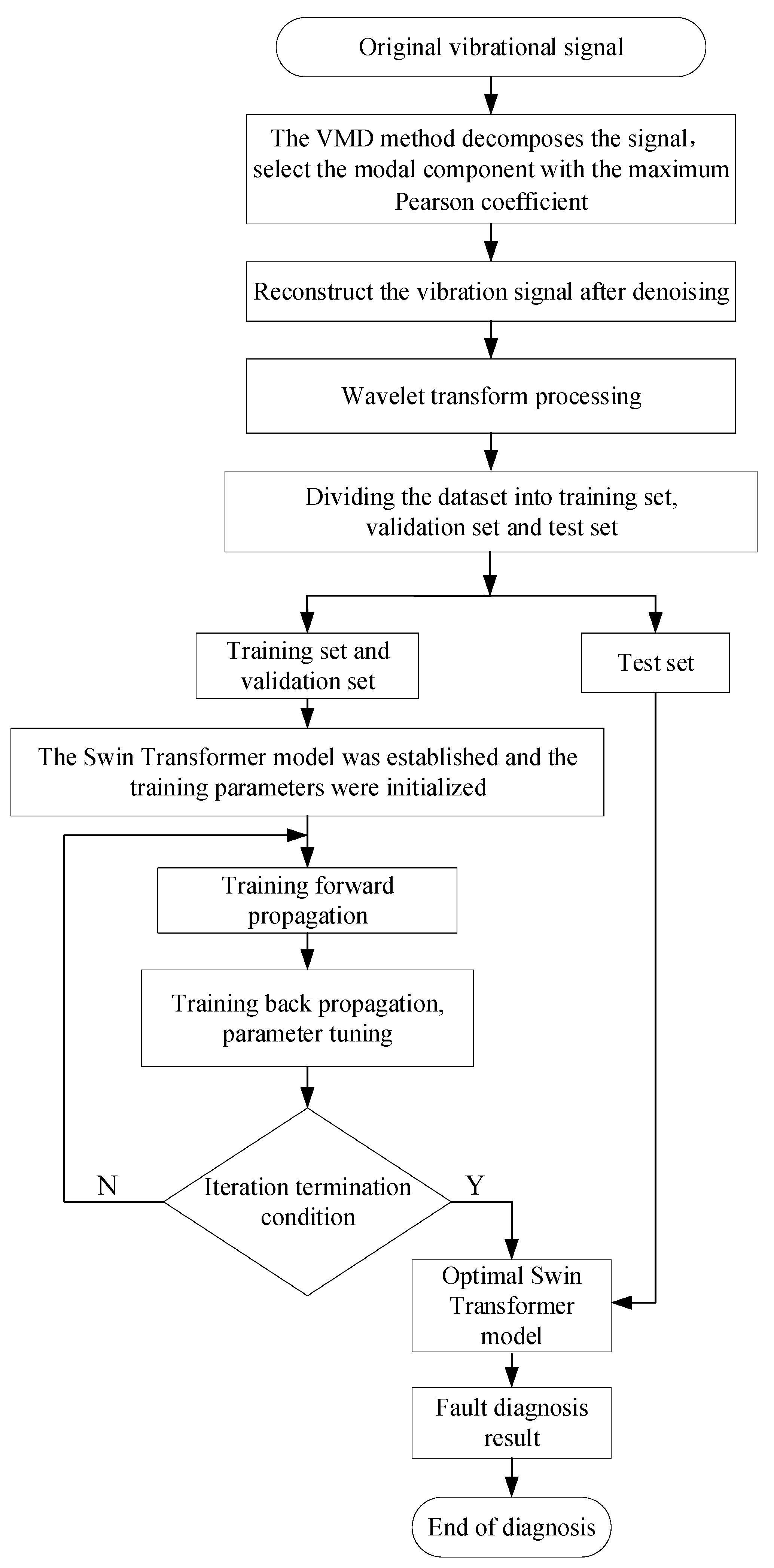
In this study, a combination of VMD and Swin Transformer was used for fault diagnosis of belt conveyor rollers. First, the VMD algorithm was used to realize signal decomposition and reconstruction. Subsequently, the wavelet transform was applied to generate time–frequency domain feature maps from the denoised and reconstructed signals. Finally, these signal spectral images were fed into a Swin Transformer network to execute feature extraction. The extracted features were finally trained using a classifier to perform fault diagnosis. For a visual representation of the workflow of the proposed method, please refer to Figure 1. The steps were as follows:

(1)

The VMD algorithm was used to decompose the signal into K modal components, and the Pearson correlation coefficient was used to select the modal component with the most significant correlation coefficient and reconstruct the denoised signal.

(2)

The denoised vibration signal was reconstructed and wavelet transform was performed to obtain the time–frequency domain feature image of the reconstructed signal.

(3)

The image was divided into training, validation, and test sets proportionally.

(4)

The training and validation sets were fed into the Swin Transformer model for training, and an optimal model was selected.

(5)

The training was terminated, and the test set was fed into the optimal model for testing.

(6)

The test results were the output.

2.2. VMD Signal Preprocessing Algorithm

The VMD algorithm operates by identifying a collection of modes along with their corresponding center frequencies, allowing these modes to recreate the input signal accurately. At its core, the algorithm expands the classical Wiener filter by incorporating multiple adaptive frequency bands. To efficiently optimize the variational model, the alternating direction multiplier method was employed to enhance the resilience of the model against sampling noise.

Assume that the real-valued signal f can be broken down into k sparse intrinsic modal components u_k. Each component u_k has its spectrum primarily concentrated within a specific bandwidth centered around ω_k. The objective of VMD decomposition is to minimize the bandwidth of each component while maintaining sparsity, essentially aiming for each modal component to be as tightly focused as possible around its center frequency ω_k. To achieve this goal, the following function is modeled [26]:

$$\underset{\left\{u_k\right\},\left\{{\omega }_k\right\}}{\min }\left\{{\displaystyle \sum _k{‖{\partial }_t\left[\left(\delta \left(t\right)+\frac{j}{\pi t}\right)\ast u_k\left(t\right)\right]e^{-j{\omega }_{k}t}‖}_2^2}\right\}$$

(1)

$${\displaystyle \sum _k{u}_k=f}$$

(2)

In Equation (1), {u_k} = {u₁, u₂,…, u_k} are the K modal components, {ω_k} = {ω₁, ω₂,…, ω_k} are the center frequencies of each component, * is the sign of convolution operation, and ∂t is the sign of gradient operation. Equation (1) can be simplified to Equation (2).

Introducing the quadratic penalty term α and the Lagrange multiplier operator λ(t), the constrained optimization problem of Equations (1) and (2) are converted into an unconstrained problem with an augmented Lagrangian function of the following form [26]:

$$\begin{array}{ll}L\left(\left\{u_k\right\},\left\{{\omega }_k\right\},\lambda \right)& =\alpha {\displaystyle \sum _k{‖{\partial }_t\left[\left(\delta \left(t\right)+\frac{j}{\pi t}\right)\ast u_k\left(t\right)\right]e^{-j{\omega }_{k}t}‖}_2^2}\\ & +{‖f\left(t\right)-{\displaystyle \sum _k{u}_k\left(t\right)}‖}_2^2+〈\lambda (t),f\left(t\right)-{\displaystyle \sum _k{u}_k\left(t\right)}〉\end{array}$$

(3)

In Equation (3), α is the penalty factor, λ(t) is the Lagrange multiplication operator, and ‹› is the inner product operation.

Once the unconstrained optimization objective function is established, the alternating direction method of multipliers (ADMM) is applied iteratively to seek optimality and determine the modal components. Initially, a set of u_k is assumed as a known condition, and the center frequency ω_k that minimizes Equation (3) is computed. Subsequently, the new center frequency ω_k is treated as a known condition, and u_k, which minimizes Equation (3), is computed. This process of alternating updates between u_k and ω_k continues until the algorithm converges or is terminated. Hence, it culminates in the determination of the optimal values for u_k and ω_k, marking the completion of the VMD decomposition process.

The VMD algorithm adaptively decomposes complex signals through iterative frequency-domain operations, resulting in multiple effective AM–FM signal combinations. This process successfully breaks down non-smooth input signals into K modal components with specific levels of sparsity. During decomposition, the choice of K is critical: selecting an excessively large value leads to over-decomposition, whereas selecting an excessively small value results in under-decomposition. To circumvent these limitations, this study employed the Pearson correlation coefficient to gauge the correlation between the decomposed signal components and the original signal, thereby determining an appropriate K value. The Pearson coefficient, denoted as γ(X, Y), is defined as follows:

$$\gamma (X,Y)=\mathrm{Cov}(X,Y)/(\sigma X\cdot \sigma Y)$$

(4)

where X and Y are two random variables, Cov(X, Y) denotes the covariance of X and Y, and σX and σY denote the standard deviation of X and Y, respectively.

The value of K is determined using the following procedure:

(1)

The initial number of modal components is set as K = 2, (K ≤ 10).

(2)

The vibration signal is decomposed using VMD.

(3)

Determine γ(u_k−1, f) ≥ γ(u_k, f), if it means that the VMD is over-decomposed, such that K = K − 1, the loop ends; otherwise, make K = K + 1, and reiterate step (2).

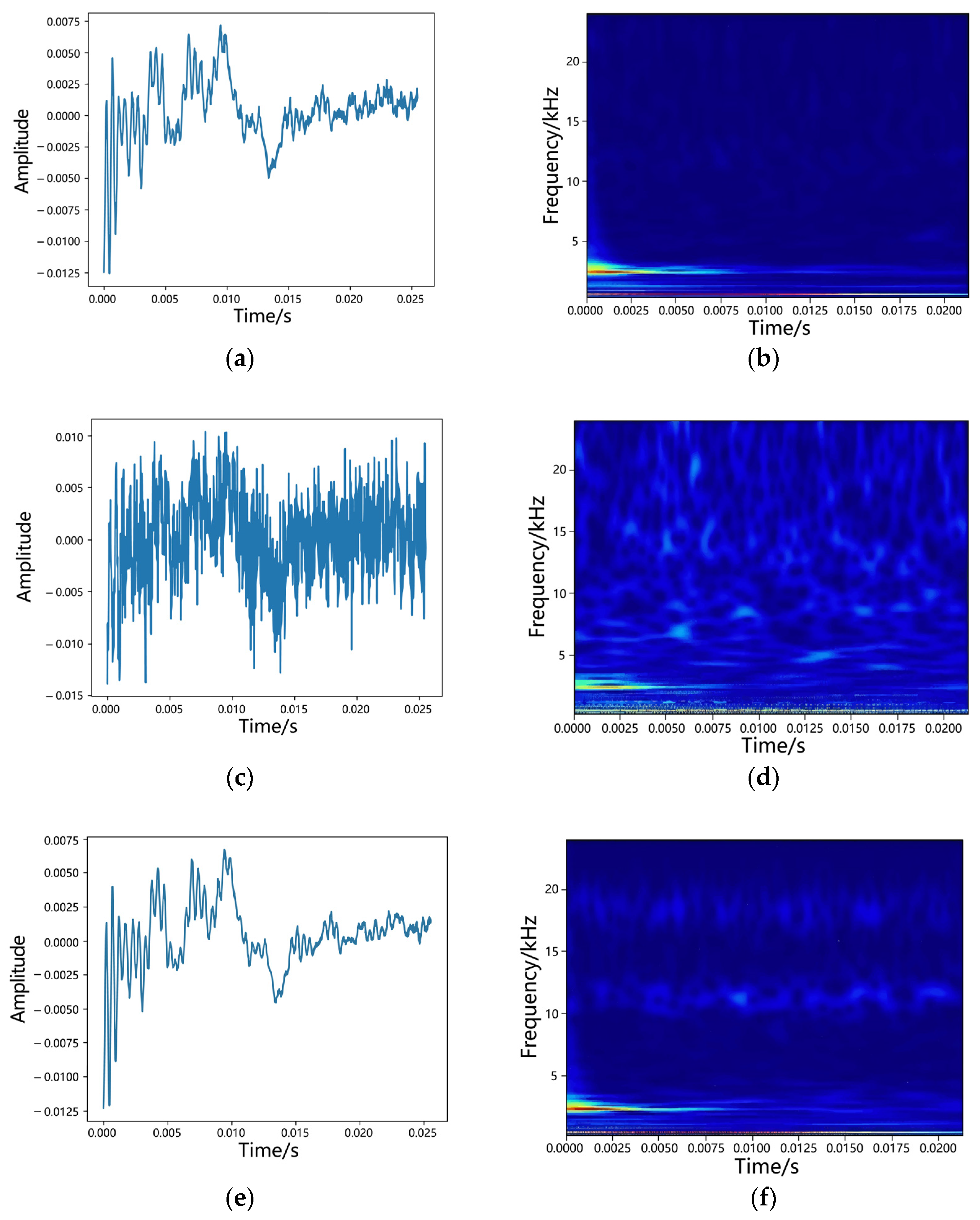
After selecting the number of modal components K, each modal component was obtained via VMD. Subsequently, the Pearson correlation coefficient between each modal component and original signal was calculated. The corresponding modal components were arranged based on these correlation coefficients, and a valid signal was reconstructed. The effect of the noise reduction on the roller-fault signal is plotted in Figure 2.

To simulate the roller’s fault data in the presence of substantial background noise, a synthetic signal was generated by combining a robust background noise component with an initial fault impulse signal (Figure 2c). The introduction of the noise component resulted in a cluttered time-domain signal, submerging the time–frequency domain characteristics of the original fault impulse signal (Figure 2d). Consequently, it is challenging to effectively distinguish fault-related time-domain features. To isolate the original vibration signal from the noise-corrupted signal, we employed a VMD signal-to-noise separation algorithm to treat the faulty signal. The time-domain waveform, which was compromised by noise, was subjected to VMD processing with a structure similar to that of the original waveform (Figure 2e). The application of the VMD algorithm diminished the noise component within the reconstructed signal spectrum, resulting in clear time–frequency domain features (Figure 2f). Examining the entirety of Figure 2, it is evident that the VMD, which functions as an adaptive signal separation method, decomposes the signal into multiple intrinsic modal components and selects the signal components that have less noise information in the modal components and are maximally correlated with the original signal to be combined. This amalgamation effectively diminishes the noise interference in the reconstituted signals while preserving crucial information. Although certain components of the time-domain signal may cancel each other out along the time axis and remain imperceptible, they become distinctly visible in the time–frequency domain. Consequently, conducting wavelet time–frequency domain analysis on the noise-reduced signal after VMD decomposition and recombination enables the precise extraction of the signal’s time–frequency domain information.

In the VMD signal-to-noise separation algorithm, the value of K is particularly important, and the initial value of K is set to two. The correlation coefficients obtained for each modal component are listed in

Table 1. Correlation coefficient of “Κ” value corresponding to each modal component.

K	IMF1	IMF2	IMF3	IMF4
2	0.421	0.590	—	—
3	0.396	0.427	0.593	—
4	0.415	0.467	0.534	0.471

.

Table 1 displays the Pearson correlation coefficients corresponding to each intrinsic mode function (IMF) resulting from decomposition. Notably, these coefficients generally increased in each group when K = 2 or 3. However, when K = 4, IMF3 surpassed IMF4; this anomaly arose primarily from the over-decomposition of the signal during decomposition. Conversely, when K was set to 2 or 3, the signal remained incompletely decomposed. Hence, to identify the optimal number of IMFs for the aforementioned simulated signal, we selected the modal component IMF3, which exhibited the highest Pearson coefficient, to reconstruct a useful signal. The effect of varying the K values on the signal-denoising performance was assessed through a sensitivity analysis of the number of modal components K. A comparative evaluation of the time–frequency domain images of the signal for the original noise-added analog signal and the reconstructed signal after VMD decomposition indicated that the VMD method greatly reduced the noise component within the reconstructed signal and enhanced the visibility of fault-related information when employing the optimized K value.

2.3. Swin Transformer Network Model Buliding

CNNs have historically been the primary networks for visual processing applications. However, with the introduction of the transformer structure by Vaswani et al. [27], featuring a global receptive field in a single layer, researchers have begun to explore its application in computer vision tasks. Remarkably, the transformer network surpassed the CNN in terms of performance on large image datasets, establishing itself as a viable alternative in the realm of computer vision. This transition has yielded impressive results across numerous computer vision tasks. Considering the vision transformer (ViT) [28] as an example, the ViT captures an image and divides it into multiple fixed-size patches. Subsequently, these patches are linearly transformed into embedding vectors that are processed by multiple encoders for feature extraction, which is a crucial step in image classification. This approach, which segments an image, excels in capturing global information from the image. However, this method exhibits limitations when extracting detailed local image information. In contrast, the Swin Transformer addresses this limitation by enabling the interaction of information across different regions of the entire segmented image. This breakthrough considerably improves the accuracy of image classification by effectively leveraging both global and local information.

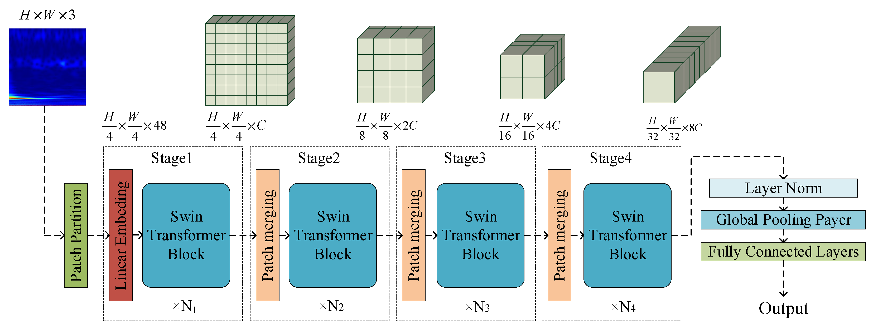
The overall architecture of Swin Transformer is illustrated in Figure 3.

The Swin Transformer network model is organized into four stages, each sharing a similar structural composition. In the initial stage, the RGB three-channel image with dimensions H × W undergoes a Patch Partition layer. This layer divides the image into non-overlapping patches of equal size, each measuring 4 × 4 and comprising three channels. Consequently, after flattening, the feature dimensions are 4 × 4 × 348. Consequently, the input sequence length for the Swin Transformer is represented by H/4 × W/4 = H × W/16 patch tokens, reflecting the effective input sequence length of the model.

The linear embedding layer, also known as a fully connected layer, is responsible for projecting a tensor with dimensions (H/4 × W/4) × 48 onto any dimension C. This transformation converts the vector dimension to (H/4 × W/4) × C and subsequently feeds the patch token into the Swin Transformer block. This block structure is illustrated in Figure 4b. In the initial Swin Transformer block, the number of input and output tokens remains unchanged at H/4 × W/4, and it collaborates with the linear embedding layer in Stage 1. However, as the network depth increases, the number of tokens decreases because of the merging process implemented by the patch-merging layer.

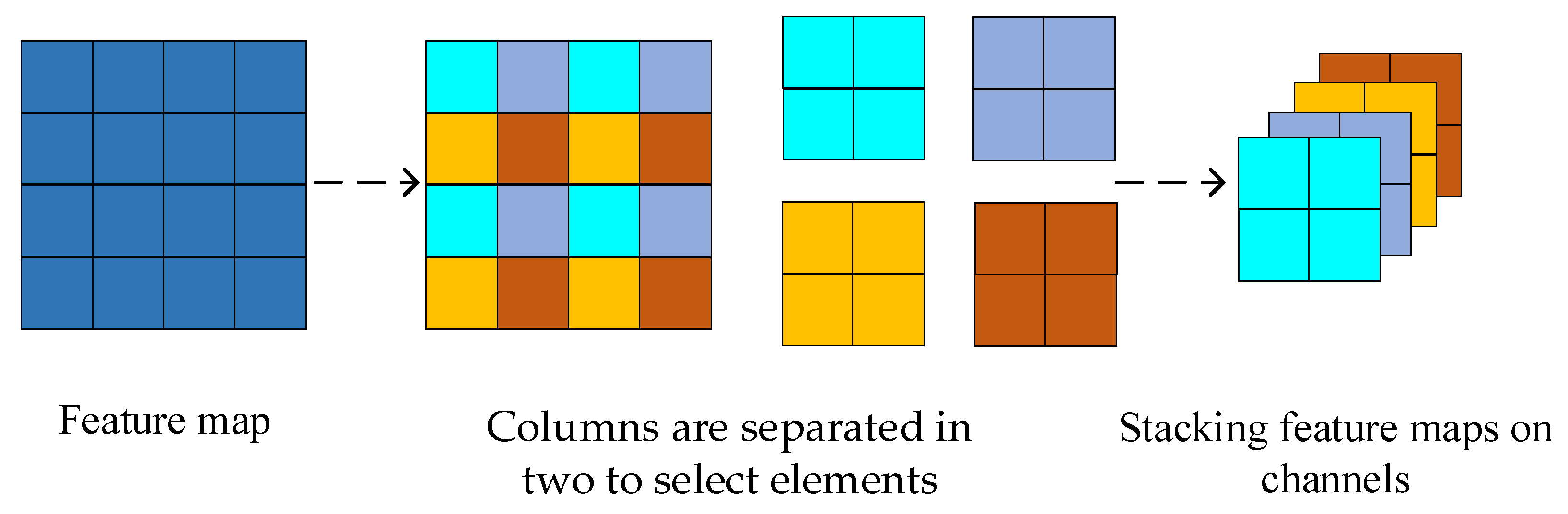
The first patch-merging layer and the Swin Transformer Block of this stage are combined to form Stage 2. The patch-merging layer splices each set of patches with an interval of two, reducing the number of patch tokens to 1/4 of the original size, i.e., H/8 × W/8. In contrast, the dimensions of the patch token expands to 4C. This process is illustrated in Figure 5. To optimize the computational efficiency, a linear layer is applied to perform dimensionality reduction on a patch with a dimension of 4C, reducing the output dimension to 2C, thereby lowering the resolution and minimizing the computational load. Following this reduction, the Swin Transformer block performs a feature transformation. Subsequently, Stages 3 and 4 replicate the same process as Stage 2, with each iteration altering the tensor dimensions to establish a hierarchical representation. In this context, N1, N2, N3, and N4 represent the numbers of Swin Transformer blocks at each stage. Typically, N1, N2, and N4 are configured as 2, whereas N3 may vary depending on the specifics of the training data.

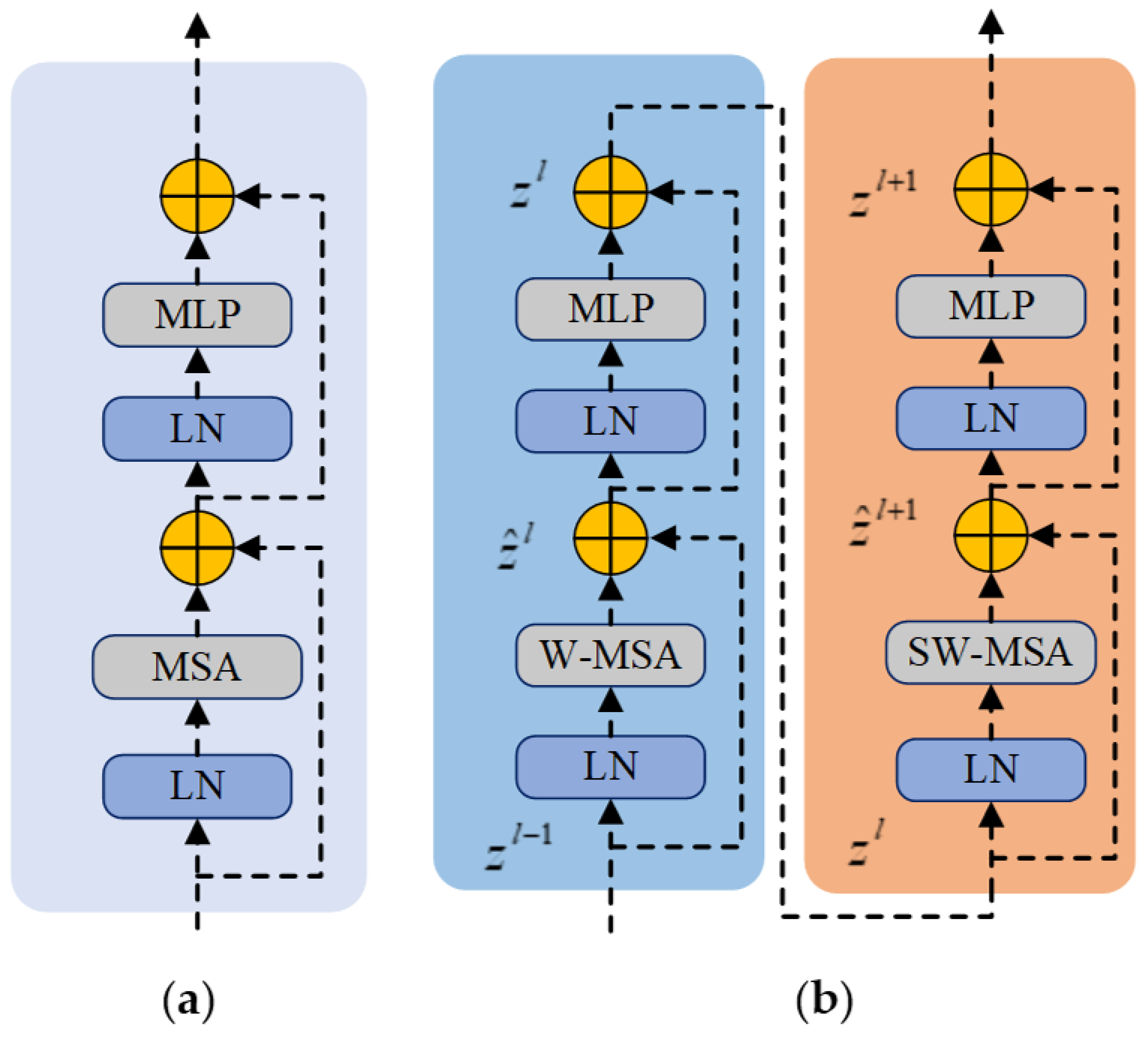
The Swin Transformer encoder closely resembles the traditional transformer encoder structure (Figure 4a), comprising a multi-head self-attention (MSA) layer, normalization (LN) module, and multilayer perceptron (MLP). The MSA layer is pivotal in extracting information from various dimensions, enhancing feature diversity, preventing overfitting, and ultimately improving the overall model performance. This layer operates by employing different attention heads with distinct Q (query), K (key), and V (value) matrices. These matrices are randomly initialized to project the input vectors into different subspaces. Multiple independent attention heads concurrently process the input, and the resulting vectors are aggregated and mapped to the final output. The mechanism of MSA is as follows [27]:

$$Q_i=X{W}^{Q_i}, K_i=Y{W}^{K_i}, V_i=Y{W}^{V_i}$$

(5)

$$Z_i=Attention(Q_i,K_i,V_i),i=1\dots h$$

(6)

$$MSA(Q,K,V)=Concat(Z_1,Z_2,\dots ,Z_h)W^O$$

(7)

where i is the number of the attention head, which ranges from 1 to h; $W^{Q_i}\in R^{d_{model}\times d_k}$, $W^{K_i}\in R^{d_{model}\times d_k}$, and $W^{V_i}\in R^{d_{model}\times d_v}$ denote three different linear matrices; $W^O\in R^{h{d}_v\times d_{model}}$ is the output projection matrix; and $Z_i$ refers to the output matrix of each attention head.$X$ and $Y$ denote the input vectors, $d_k$ refers to the dimensions of query and key, and $d_v$ refers to the dimension of value. The MSA separates the inputs into h-independent attention heads under the action of the $d_{model}/h$-dimensional vectors and performs multi-head parallel processing of the features. The processed vectors are mapped to the final output using aggregation, which is performed using the $Concat$ function.

As plotted in Figure 4a, the encoder consists of two segments of residual link structures that enhance the flow of image information and contribute to the improved model training accuracy. A common functional module of LN is used within each residual link. The attention mechanism is applied to the first residual link, whereas in the second residual link, the MLP function formula is expressed in Equation (8) [27].

$$MLP(x)=\sigma (W_{1}x+b_1)W_2+b_2$$

(8)

The two linear transformation layers with a non-linear activation function from the MLP structure, $W_1$ and $W_2$ in the aforementioned equation, are the parameter matrices of the two linear transformation layers. The activation function is usually a Gaussian error linear unit function, denoted by $\sigma$ in Equation (8), where $b_1$ and $b_2$ are bias parameters.

The Swin Transformer block, as depicted in Figure 4b, comprises two encoders connected in series. Essentially, the encoder structure within the Swin Transformer Block remains unchanged compared to the standard transformer encoder, with the exception that the MSA is substituted with window-based window multi-head self-attention (W-MSA). In addition, shifted-window multi-head self-attention (SW-MSA), which is based on the shifted window while retaining other unaltered components, is introduced. Unlike MSA, W-MSA and SW-MSA specifically concentrate on attentional relationships within local windows, resulting in lower computational complexities. However, all three share the same fundamental principles. Furthermore, the structure and function of the LN layer and the MLP module mirror those of the transformer.

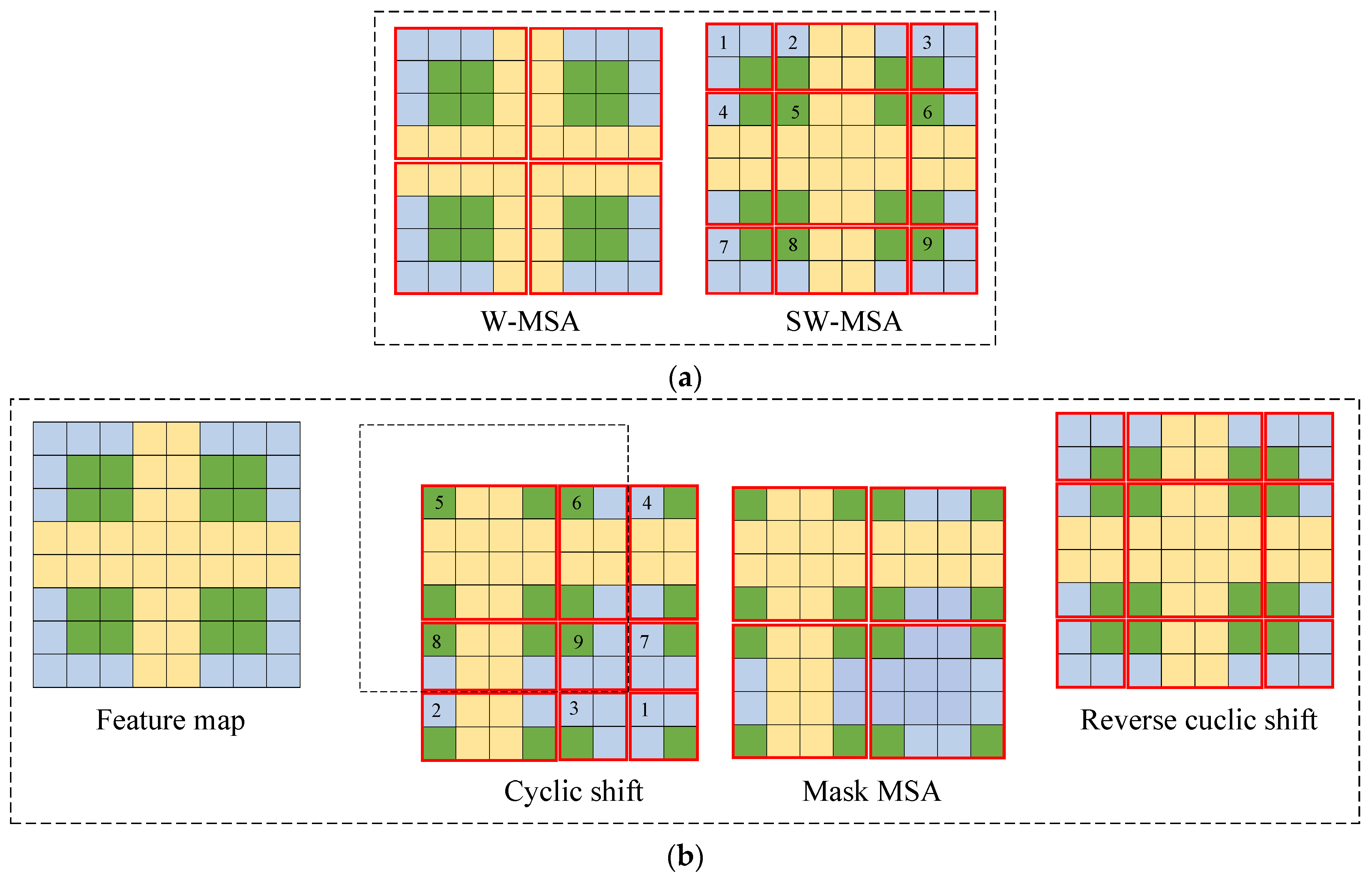
As illustrated in Figure 6a, a typical MSA structure involves numerous computations for each element in the feature map. The W-MSA module reduces the computational load by segmenting the feature map into windows of size M × M and separately conducting self-attention computations within each window. In contrast to the conventional windows of the W-MSA, the SW-MSA module utilizes shifted windows to expand the receptive field. Figure 6a illustrates the transformation of the four W-SMA windows into nine SW-MSA windows. The process of shifting the windows is illustrated in Figure 6b. Post-shift, the batch window count remains unchanged; however, certain windows may contain content from the sub-windows that were initially non-adjacent. Hence, the Mask MSA mechanism is initially employed for self-attention calculations. Subsequently, a Mask operation is executed to eliminate undesired attention, confining self-attention calculations to sub-windows that require MSA calculations. This enables the model to concentrate solely on specific location information, while disregarding irrelevant location details. Finally, the shift operation is iterated to retrieve the self-attention outcome for a specific window. For instance, in Figure 6b, only window 5 requires no splicing, resulting in the preservation of only the MSA results for this window. W-MSA and SW-MSA were performed in tandem. For instance, regular window segmentation was applied in the l-th coding layer, whereas the l + 1th layer utilized a shifted-window approach. This method involving shifted-window segmentation establishes connections between adjacent non-overlapping windows from the previous layer, enhancing the linkage between local features and bolstering the accuracy of the Swin Transformer in image classification.

The specific formulas for calculating the Swin Transformer Block are as follows [21]:

$${\widehat{z}}^l=W-MSA(LN(z^{l-1}))+z^{l-1}$$

(9)

$$z^l=MLP(LN({\widehat{z}}^l))+{\widehat{z}}^l$$

(10)

$${\widehat{z}}^{l+1}=SW-MSA(LN(z^l))+z^l$$

(11)

$$z^{l+1}=MLP(LN({\widehat{z}}^{l+1}))+{\widehat{z}}^{l+1}$$

(12)

where ${\widehat{z}}^l$ and $z^l$ denote the output characteristics of the l-layer encoder W-MSA and MLP modules, respectively, and ${\widehat{z}}^{l+1}$ and $z^{l+1}$ denote the output characteristics of the l + 1-layer encoder SW-MSA and MLP modules, respectively. $W-MSA$ and $SW-MSA$ refer to W-MSA and SW-MSA operations, and $LN$ denotes the Layer Normalization function.

3. Fault Diagnosis Accuracy Test

To validate the effectiveness and accuracy of the proposed method, we conducted tests to evaluate its signal-noise reduction capability and fault-recognition accuracy using a roller failure dataset.

The roller failure dataset encompassed various fault types, including roller surface cracks, roller surface wear, roller jamming, abnormal roller vibration, and a category representing normal rollers. To prevent the model from overfitting problems during training and testing, and to ensure the accuracy of the test results, the number of test sets should not be too large. Therefore, the fault datasets of different fault types were divided into training, validation, and test sets at a ratio of 7:2:1. The selection information is presented in

Table 2. Roller failure dataset.

Fault Type	Sample Size	Categery Label
Normal	200	0
Roller surface crack	200	1
Roller surface wear	200	2
Roller stuck	200	3
Roller abnormal vibration	200	4

.

Gaussian white noise was introduced into the original data samples to simulate noise-affected data and assess the diagnostic performance of the proposed algorithm on noisy data. The signal-to-noise ratio (SNR) was calculated as follows:

$$R_{sn}=10\lg \left(\frac{p_{signal}}{p_{noise}}\right)$$

(13)

where R_sn denotes the SNR, P_signal denotes the effective power of the signal, and P_noise denotes the effective power of noise.

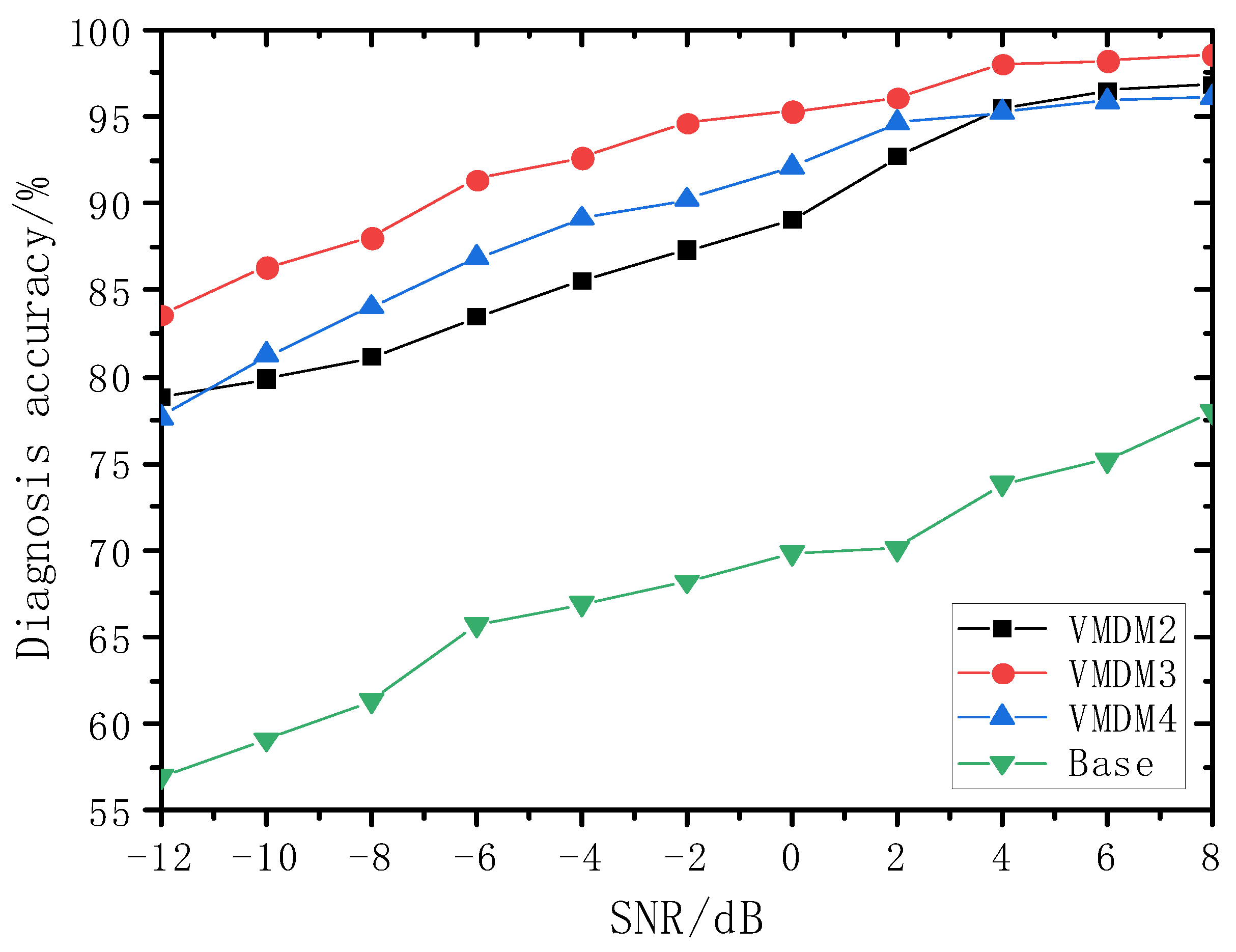
To study the impact of the proposed improved VMD method on the fault identification accuracy, the original noise-added signal (strong background noise superimposed on the original signal) and three groups of signals obtained from the improved VMD decomposition were selected and fed into the swine transformer for fault comparison. The three sets of decomposed input signals can be categorized as follows: (i) contains two modal components corresponding to the maximum Pearson correlation coefficient (i.e., maximum value), K = 2 (denoted as VMDM2); (ii) contains three modal components corresponding to the state component with the most significant Pearson correlation coefficient (i.e., state component), K = 3 (denoted as VMDM3); and (iii) contains four modal components corresponding to the maximum Pearson correlation coefficient (i.e., maximum value), K = 4 (denoted as VMDM4). The number of Swin Transformer blocks in each stage of the Swin Transformer network structure for the four types of models was two, two, six, and two, respectively. The test results are presented in Figure 7. The signal recognition accuracies achieved by the four models varied at different SNR levels. At an SNR of 0 dB, the accuracies stand at 89.02%, 95.30%, 92.08%, and 69.82%, respectively; however, these values dropped to 78.85%, 83.60%, 77.65%, and 56.98%, respectively, when the SNR dropped to −12 dB. Among the four groups of input signals, those with a signal component of three consistently exhibited higher fault recognition accuracy compared to the other three groups. Notably, when utilizing the three most significant signal components, the accuracy of the model experienced a more gradual decline as the noise levels increased. This trend suggests that the recognition accuracy of the model was less susceptible to changes in the SNR. This observation underscores the importance of selecting an appropriate K value during signal decomposition, as variations in K can lead to either under-decomposition or over-decomposition of the signal, both of which can adversely affect the model accuracy. Thus, selecting the right K value is essential for achieving a high model accuracy.

To make the Swin Transformer model more adapted to the VMD method, the number of Swin Transformer coding layers was adjusted to test the accuracy of Swin-T, Swin-S, and Swin-L on the test set separately. Swin-T, Swin-S, and Swin-L differred mainly in terms of the output feature map dimension C and number of Swin transformer blocks N3 in Stage 3. The parameters of each model are listed in

Table 3. Parameters for various Swin Transformer models.

Models	Image Size	C	N1	N2	N3	N4
Swin-T	224 × 224	96	2	2	6	2
Swin-S	224 × 224	96	2	2	18	2
Swin-L	224 × 224	192	2	2	18	2

.

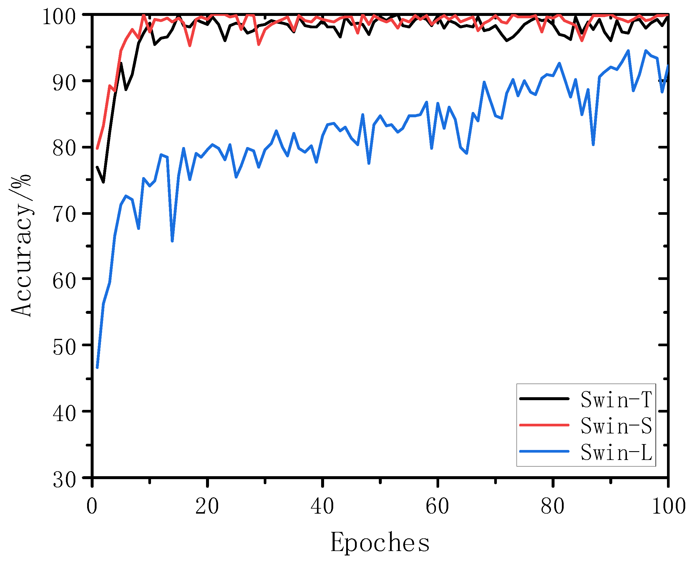
The training accuracies of the three Swin Transformer models for the classification and recognition of the established validation set are illustrated in Figure 8. An in-depth analysis of the results revealed that Swin-T and Swin-S demonstrated faster convergence and higher accuracy as the iterations progressed. In contrast, the Swin-L model exhibited a considerably lower classification accuracy for the validation set. The accuracy of the Swin-T and Swin-S models quickly rose to over 95% and reached a maximum of 99.6% and 99.3%, respectively, while the Swin-L model reached a maximum of 93.8%. In particular, the accuracy curve exhibited more pronounced fluctuations, indicating sub-optimal convergence. Two primary factors contributed to this phenomenon. First, the Swin-L model was inherently more complex than the Swin-T and Swin-S models because of its larger feature map dimensions (C) and greater number of coding layers. This led to an elevated computational demand for the training process. Second, the size of the validation dataset remained constant throughout training, which could lead to overfitting and consequent fluctuations in the accuracy curves across different training rounds.

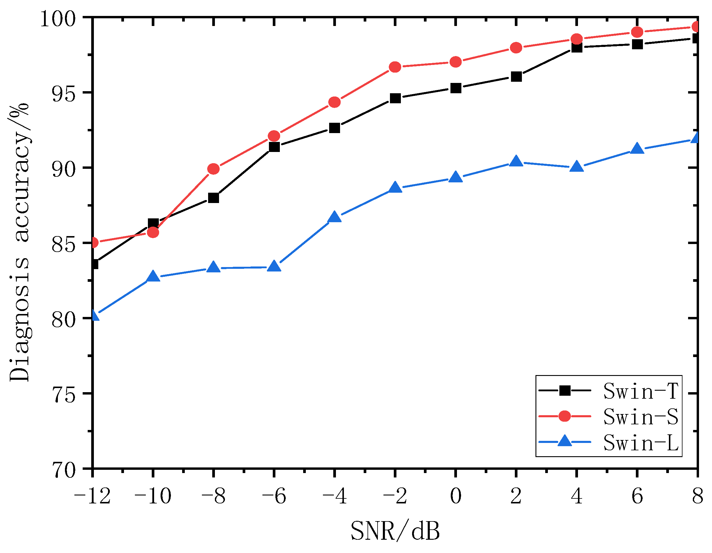
The sample data covered an SNR range from −12 dB to 8 dB. After decomposing and reconstructing the signal components using VMDM3, they were fed into a Swin Transformer for analysis. The test results are plotted in Figure 9. As the SNR gradually increased, there is a noticeable decrease in the performance of the Swin-L model. Throughout the SNR variations, the diagnostic accuracy curves of the Swin-T and Swin-S models exhibited similar trends, with the Swin-S model consistently achieving a slightly higher accuracy than the Swin-T model. Notably, at an SNR of 0 dB, the Swin-L, Swin-T, and Swin-S models’ test accuracies were 89.3%, 95.3%, and 97.02%, respectively, at which time the accuracy of the Swin-S model was 7.72 and 1.72 percentage points higher than that of the Swin-L and Swin-T models, respectively. At an SNR of 8 dB, the accuracy of the Swin-L, Swin-T, and Swin-S models’ tests was 91.9%, 98.6%, and 99.3%, respectively, at which time the accuracy of the Swin-S model was 7.2 and 0.7 percentage points higher than that of Swin-L and Swin-T, respectively. Examining Figure 8 and Figure 9 collectively, it is evident that Swin-L exhibited a consistently low and fluctuating accuracy during training. This result is attributed to the excessively complex model structure and computational demands. In contrast, the Swin-T and Swin-S models outperformed the Swin-L model on the test set owing to their simpler architectures and more manageable computational requirements. Comparing the Swin-T and Swin-S models, the latter’s strategy increased the number of encoders in Stage 3, resulting in a greater model complexity. Notably, the Swin-S model demonstrated a superior test accuracy compared to the Swin-T model. This discrepancy can be attributed to the distinct architectures of the Swin-S and Swin-T models, which could affect their feature extraction capabilities. With a greater number of coding layers, the Swin-S model excelled in hierarchical feature representation, enabling it to capture information at various scales within an image. However, the Swin-L model experienced a decline in accuracy despite an increase in model complexity. This decline is attributed to the oversized structure of the Swin-L model, resulting in overfitting, in which the model learns numerous noisy or redundant features from the training data that cannot be effectively applied to the test data. Moreover, all three models shared the same dataset, and large-scale models typically require greater computational resources and more refined training strategies for convergence and generalization. Performance degradation can be prevented by allocating additional resources and implementing suitable training strategies for the Swin-L model.

In summary, the increased complexity of the Swin-S model, coupled with its higher accuracy, was likely a result of determining the optimal equilibrium between the model size and training strategy, enabling it to capture data patterns more effectively. Conversely, despite its greater complexity, the Swin-L model exhibited lower accuracy owing to challenges stemming from issues such as sub-optimal architectural design, overfitting, and inadequate training resources.

The ViT, similar to the Swin Transformer, is a variant of the transformer model designed for processing two-dimensional data by incorporating internal encoders equipped with attention mechanisms. The primary distinction lies in the image-processing approach. When ViT receives an image, it directs it through multiple encoders for feature extraction, employing the MSA mechanism to capture the features of the entire image. In contrast, the encoding module of the Swin Transformer introduces a hierarchical processing mechanism that comprises W-MSA and SW-MSA. W-MSA focuses on extracting features from different parts of an image, whereas SW-MSA cascades the features across various image regions. Consequently, the ViT primarily emphasizes global feature extraction, whereas the Swin Transformer excels in capturing both local and global features.

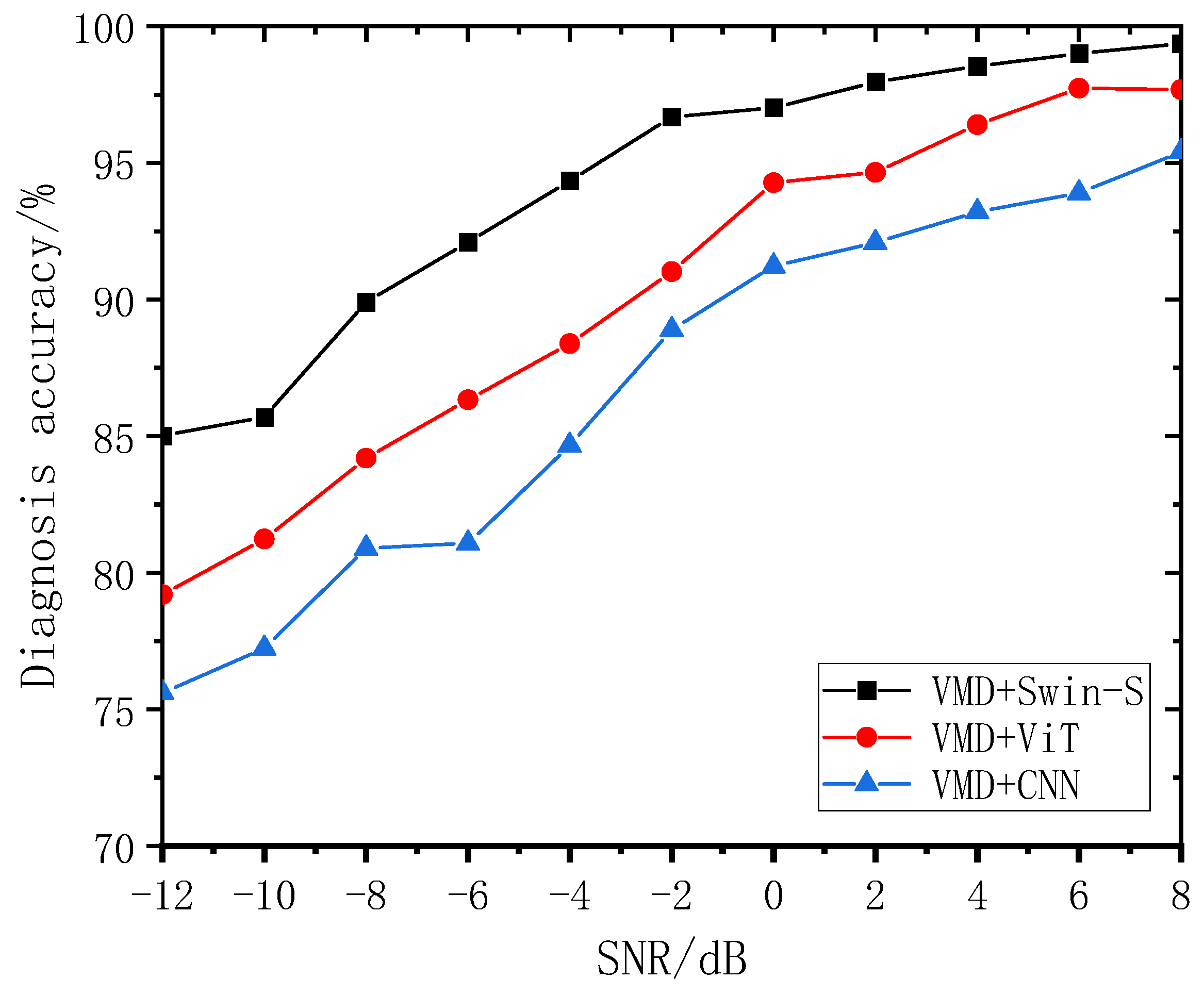
To evaluate the fault recognition accuracy of the proposed methods in the presence of high background noise, we benchmarked our approach against the VMD + CNN [29] and VMD+ViT [30] networks. In this direction, we performed a comparative analysis of fault diagnosis accuracies across a range of SNRs (−12 dB to 8 dB), as illustrated in Figure 10. Notably, for VMD + CNN, the recognition accuracy started at 75.6% when the SNR was at its lowest (−12 dB) value and achieved its highest accuracy of 95.40% at an SNR of 8 dB. In contrast, VMD+ViT exhibited a recognition accuracy of 79.20% at an SNR of −12 dB, which subsequently rose to 97.68% at an SNR of 8 dB. Furthermore, in the SNR environment ranging from −12 dB to 8 dB, the accuracy of the VMD+Swin-S model demonstrated a remarkable improvement, rising from 85.02% to 99.36%. Thus, among the three methods evaluated for noise resilience, VMD+Swin-S emerged as the best performer, followed by VMD+ViT, and VMD + CNN exhibited the lowest robustness. The main characteristics of the three models and their performance in the test are shown in

Table 4. Comparison of characteristics and test accuracy of three models.

Models	Input Data Dimensions	Feature Extraction	Highest Accuracy in the Test
VMD + CNN	One-dimensional	Local feature	95.40%
VMD+ViT	Two-dimensional	Global feature	97.68%
VMD+Swin-S	Two-dimensional	Global and local features	99.36%

.

According to Table 4 and Figure 10, it can be seen that this performance difference can be attributed to the inherent features of these models. For example, the input data of the CNN model was one-dimensional, while the ViT and Swin Transformer are used to process two-dimensional data; compared with one-dimensional data, two-dimensional data can show richer features, and in terms of the feature input, the ViT and Swin Transformer gain more advantages than a CNN. In addition, a CNN is primarily designed for extracting local features and struggles to capture distant features in input time-series data. In particular, when dealing with long sequences of sound vibration signal data, CNNs often require layer-by-layer convolution operations, leading to a proliferation of parameters and computations. In contrast, the ViT model incorporates the MSA mechanism, enabling it to capture global features and discern the varying contributions of different samples to the results. This capability enables the VMD+ViT method to achieve superior fault diagnosis performance. In contrast to the ViT and CNN, the Swin Transformer incorporates a hierarchical processing approach involving window-based W-MSA and SW-MSA. This methodology divides an image into localized regions, applies a self-attention mechanism to each region, and subsequently propagates information through a hierarchical structure. This hierarchical processing enhances the model’s ability to capture the local features of the image while effectively processing global information through the synergy of local attention and the hierarchical structure. Consequently, this approach enables the Swin Transformer to comprehensively grasp the intricate features within an image and establish relationships among localized elements, resulting in an improved diagnostic performance. The model’s adeptness in balancing local and global information extraction positions the Swin Transformer as a superior choice compared to the ViT and CNNs in the realm of diagnosis. The disadvantage of taking into account both global and local features is the more complex structure of the model, so the simpler structure of CNNs and the ViT will be more advantageous in terms of the efficiency of model operation.

4. Application Example Validation

In this paper, an industrial field faulty belt conveyor roller sound dataset was used to verify the feasibility of the proposed method in practical applications. The types of faults in the test included rusted rollers, abnormal vibrations of rollers, severe cracking of the belt, and normal rollers. The applied rotational speeds during the test were 50 r/min, 200 r/min, and 400 r/min, respectively. The dataset was divided into training, validation, and test sets at a ratio of 7:2:1, and this was inputted into five types of models for the test, namely, VMD+Swin-S, VMD+Swin-T, VMD+Swin-L, and VMD+ViT with VMD + CNN. The test results are shown in Figure 11.

From Figure 11, it can be seen that the VMD+Swin-S model had the highest accuracy among all the models at working speeds of 50 r/min, 200 r/min, and 400 r/min with 98.67%, 98.32%, and 97.65% accuracy, respectively. The accuracy of the VMD+Swin-T model was close to that of the VMD+Swin-S model, with 98.05%, 96.3%, and 96.22% accuracy, respectively. The accuracy of both models was ahead of other models under all types of working conditions. The fault diagnosis effect of the VMD+ViT model was better than that of the VMD + CNN model as a whole. Among all the models, the VMD+Swin-L model had the lowest accuracy under three types of working conditions, and the accuracy of this model was only 79.2% under a rotational speed of 400 r/min. According to the analysis shown in Figure 9, it can be seen that this was caused by the model being too complex and an overfitting problem being present. Based on the above results, it can be seen that the VMD+Swin-S model still had a high accuracy under practical applications.

5. Conclusions

In addressing the challenge of diagnosing belt conveyor roller faults in noisy environments, this paper presents a method that utilizes the VMD and Swin-S model for accurate fault diagnosis of roller sound signals. The following conclusions are drawn from the tests conducted on belt conveyor roller sound data:

(1)

The optimization of parameters for the VMD and Swin Transformer models can be tailored to specific application scenarios. The VMD signal decomposition and reconstruction method, incorporating modal components with the three highest Pearson correlation coefficients, when combined with the Swin Transformer variant structure Swin-S, demonstrates superior diagnostic accuracy in noisy environments.

(2)

The VMD+Swin Transformer model proved to be very effective in fault diagnosis, even in the presence of large amounts of noise. By adjusting the parameters of the coding layer of the Swin Transformer, the accuracy of the VMD+Swin-S model reached 99.36% when testing the drum with centralized sound data, highlighting its precision and robustness. The accuracy of the VMD+Swin-T model also reached 98.6%.

(3)

In various noise condition tests, the accuracy of the VMD + CNN and VMD+ViT methods was 95.4% and 97.68%, respectively. The VMD+Swin-S model proposed in this paper was better than the VMD + CNN and VMD+ViT methods in terms of its fault diagnosis accuracy of belt conveyor rollers. In the example application test, the accuracy of the VMD+Swin-S model at the three rotational speeds was 98.67%, 98.32%, and 97.65%, respectively, which was the highest among the models compared. This approach is well-suited for the precise diagnosis and classification of fault categories in belt conveyor rollers operating in strong noise environments.

In this study, VMD was combined with Swin-S to obtain an optimal model that can recognize roller faults in a strong noise environment. However, the principle of the Swin Transformer model is more complicated, and its application on large-scale images may face the challenge of computational and storage resources. Therefore, lightweighting the Swin Transformer model and optimizing the computational efficiency and the number of parameters of the Swin Transformer, while ensuring the testing accuracy of the model for more efficient training efficiency and diagnostic accuracy, can be a direction for further research.