


Analyzing Distance-Based Registration with Two Location Areas: A Semi-Markov Process Approach
Department of Industrial & Information Systems Engineering and the RCIT, Jeonbuk National University, 567, Baekje-daero, Deokjin-gu, Jeonju-si 54896, Republic of Korea
Electronics 2024, 13(1), 233; https://doi.org/10.3390/electronics13010233
Submission received: 30 November 2023
/
Revised: 28 December 2023
/
Accepted: 2 January 2024
/
Published: 4 January 2024
(This article belongs to the Topic Electronic Communications, IOT and Big Data)
Abstract
:In order to connect an incoming call to the user equipment (UE) in a mobile communication network, the location information of the UE must be always kept in the network database. Therefore, the efficiency of the location registration method of reporting new location information to a mobile communication network whenever the location information of the UE changes directly affects the performance of the radio channel, which is a limited resource in a mobile communication network. This study deals with distance-based registration (DBR). DBR does not cause the ping-pong phenomenon known to be a main problem in zone-based registration. It shows good performance when assuming a random walk mobility model. To improve the performance of the original DBR with one location area (1D), a DBR with two location areas (2D) was proposed. It is known that 2D is better than 1D in most cases. However, unlike 1D, an accurate mathematical model for 2D has not been presented in previous studies, raising questions about whether an accurate performance comparison has been performed. In this study, we present an accurate mathematical model based on the semi-Markov process for performance analysis of 2D. We compared performances of 1D and 2D using the proposed mathematical model. Various numerical results showed that 2D with two-step paging was superior to 1D in most cases. However, when simultaneous paging was applied to 2D, 1D was better than 2D in most cases. In real situations, optimal performance can be achieved by reflecting the network situation in real time and dynamically changing the operating method using a better-performing model among these two methods.
1. Introduction
In a mobile communication network, the user equipment (UE) has the ability to move freely. Thus, the network must know the location information of the UE in order to connect a call to the UE. Location registration refers to the process by which the UE will report location information that changes depending on its movement to the network. When an incoming call occurs to a UE, the network finds the UE location information in its database and sets up the call based on that information. Since the efficiency of these location registration schemes directly affects the overall efficiency of radio resource management, it is important to find the optimum registration method.
Many proposals for location registration have been put forward, such as zone-based registration (ZBR) [1,2,3], distance-based registration (DBR) [1,4,5,6,7,8,9], movement-based registration [8,9,10,11], and time-based registration [1]. Movement-based registration has been discussed thoroughly in the literature, but its performance is not ideal. Time-based registration is only possible as an auxiliary method because it is very difficult to set the location area (LA). Thus, ZBR and DBR emerge as the most practical methods for actual mobile communication networks.
Although many studies including tracking area list-based registration and distributed mobility management for 4G/5G/6G have been performed in recent years [12,13,14,15,16,17], this method is not a completely new one but rather a flexible strategy that can be implemented in the same way as one of the traditional methods.
ZBR is used universally over all mobile communication networks and has become the focus of much research. Also noteworthy is that research on maintaining two or three LAs in ZBR instead of one has attracted attention [2,3]. International standards stipulate that the number of LAs in ZBR should equal TOTAL_ZONES (TOTAL_ZONES = 1, 2, 3, …) [1], but all mobile communication networks are run with a single LA in ZBR for convenience. Setting the number of LAs to two or three lowers location registrations but sends paging costs soaring, so research seeks to find the optimal tradeoff for minimizing total signaling costs.
In this study, we dealt with distance-based registration (DBR), another typical method applicable to the actual network. In DBR, whenever a UE enters a new cell, the distance from the most recently registered cell to the cell it just entered is calculated. If the distance is greater than or equal to the distance threshold D, location registration is performed. DBR offers advantages, including minimizing the ping-pong phenomenon associated with ZBR and distributing location registration costs evenly across all cells in the mobile communication network.
Furthermore, DBR allows a dynamic location registration method by varying the distance threshold for DBR for each UE depending on the characteristics of the UE. In addition, the performance can be improved using the effects of implicit registration by outgoing calls, which is not applicable in ZBR. In fact, DBR, along with ZBR, is one of the typical registration methods recommended by mobile communication standards [1] and is known to have as good a performance as ZBR [4].
To improve the performance of DBR with one LA (1D), DBR with two LAs (2D) has been proposed, demonstrating superior results in most cases [6]. In 2D, the UE stores not only the most recently registered LA but also the LA registered just before. In this case, location registration is not necessary when crossing two stored LAs. But this is at the cost of relatively higher paging costs than the existing 1D method. Whether to use one method or the other depends on the balance between reduced costs of location registration and increased paging costs.
However, while many mathematical analysis studies on 1D have been presented [4,5,6,7], an accurate mathematical model for 2D has been lacking, raising questions about the accuracy of the performance comparisons.
This study presents an accurate mathematical model to analyze the performance of 2D for the first time. A semi-Markov process model was used, assuming a two-dimensional random walk mobility model in a hexagonal cell environment. We showed that the proposed mathematical model could accurately evaluate performance and used this mathematical model to show which method is superior in which environment from numerical results for various environments.
The structure of this paper is as follows: Section 1 introduces the study, Section 2 explains 1D and 2D and describes the network environment for analysis, Section 3 assumes a mobility model based on a two-dimensional random walk model and presents the total signaling cost on radio channels using a semi-Markov process model, Section 4 provides numerical results for various environments, and Section 5 concludes the paper.
2. Distance-Based Registration (DBR)
Let us consider a DBR with one LA (1D) and a DBR with two LAs (2D). First, let us take a brief look at original DBR.
2.1. Distance-Based Registration with one Location Area (1D)
In DBR, whenever a UE enters a new cell, the distance between the current cell (X, Y) and the most recently registered cell (Xreg, Yreg) is calculated. If the value is greater than or equal to the distance threshold D, location registration is performed. In other words, location registration is performed if the following relational expression is satisfied [4,6]:
In real situations, the distance between two points must be accurately calculated according to changes in latitude and longitude, reflecting that the Earth is spherical [1]. However, in this study, it was sufficient to use the distance between two points on a plane.
Using DBR has several advantages [4,5,6,7]. First, new location registration occurs only after moving at least D distance from the point where the previous location registration occurred. Thus, unlike zone-based registration, a ping-pong phenomenon does not occur in DBR while moving back and forth across LA boundaries. Additionally, in DBR, each UE has a different LA. Thus, the location registration cost is generated equally across all cells in the mobile communication network. However, in a zone-based registration, the location registration cost is concentrated only on border cells of the LA.
In addition, a dynamic location registration method that can minimize the total signaling cost is possible by varying the distance threshold for DBR for each UE depending on the characteristics of the UE or by varying the distance threshold depending on the situation even for the same UE.
Another important advantage is that when an outgoing call or incoming call occurs in DBR, the same effect as location registration can be achieved without additional location registration costs [4,6]. In other words, location information can be transmitted to the network without a separate location registration message by using a call processing message to connect a call. Location registration through this procedure is called implicit registration. In location registration methods with different LAs for each UE (such as DBR, movement-based registration, and time-based registration), the outgoing or incoming call can reduce the location registration cost. When an outgoing or incoming call is attempted, the same effect can be seen as if the location is registered in the corresponding cell without additional location registration costs. Thus, the more frequently outgoing or incoming calls occur, the more the location registration cost decreases. In particular, if outgoing calls occur frequently, the number of location registrations decreases accordingly without paging occurrence. On the other hand, the generation of an incoming call can reduce the number of location registrations. However, the number of paging to find the UE increases accordingly. Therefore, considering the trade-off relationship between location registration and paging, the value of the optimal distance threshold (or the size of the optimal LA) will have to be decided.
2.2. Distance-Based Registration with Two Location Areas (2D) [6]
Let us now look at DBR with two LAs (2D), which is the main subject of this study. To evaluate the performances of 1D and 2D, assume a mobile communication network consisting of hexagonal cells of the same size as shown in Figure 1. The distance threshold D between two cells was defined as the minimum number of cells entering to move from one cell to the remaining cell for convenience. For example, in Figure 1, the distance between a ring 0-cell and one of the ring 2-cells was 2. As could be seen in the figure, in 1D with distance threshold D, an LA consisted of D rings (ring 0, 1, …, D − 1). The total number of cells in an LA was 1 + 3D(D − 1). Figure 1 shows LAs when the distance threshold D was 3.
In the 1D, when the UE performed location registration, the previous LA was deleted. That is, in the case of 1D, one LA was most recently registered. Even if the UE returned to the LA it belonged to just before entering the current LA (most recently registered), location registration must be performed anew. For example, consider the case shown in Figure 1. Let us assume that after registering the location in cell A, the UE continued to move and perform location registration in cell B. In this case, cell A was the center cell of the LA to which it belonged just before the last location registration. As shown in Figure 1, when the UE registered at cell B moved along the movement path of 1-2-3-4-5-6, in the case of 1D, the location registration should be performed at position 6, even though cell A was the cell of the LA to which it had previously belonged.
To reduce such unnecessary location registration, this study considered a DBR with two LAs (2D) [6] that could store not only the current LA but also the immediately preceding LA so that location registration would not be performed when re-entering these LAs. However, the paging cost increases compared to the existing 1D. Thus, which method has better performance can be determined depending on the decrease in location registration cost and the increase in paging cost.
In 2D, when the UE enters a new cell, distances between the current cell and center cells of the two stored LAs must both reach the distance threshold D to perform location registration.
Let LA1 and LA2 be the current LA and previous LA. In addition, let (X1, Y1) and (X2, Y2) be the coordinates of the center cells of LA1 and LA2. The 2D is operated as follows [6]:
- (1)
- When a UE is turned on, it performs a power-on registration. UE stores the current cell (X0, Y0) as the center cell of LA1.LA1: (X1, Y1) = (X0, Y0)
- (2)
- When UE enters a neighboring cell (X, Y), it calculates the distance between the current cell and LA1.
- (3)
- If UE’s distance reaches D, UE registers its location. Otherwise, it goes to step 2. After a registration, LA1 and LA2 are updated.LA2: (X2, Y2) = (X1, Y1)LA1: (X1, Y1) = (X, Y)
- (4)
- When UE enters a neighboring cell (X′, Y′), it calculates the distance between the current cell and LA1 and the distance between the current cell and LA2.
- (5)
- When both calculated distances reach D at the same time, UE registers its location. Otherwise, it goes to step 4. After a registration, LA1 and LA2 are updated.LA2: (X2, Y2) = (X1, Y1)Go to step 4.LA1: (X1, Y1) = (X’, Y’)
- (6)
- When a call occurs in cell (X″, Y″) in any of the above steps, LA1 and LA2 are updated by an implicit registration.LA2: (X2, Y2) = (X1, Y1)LA1: (X1, Y1) = (X”, Y”)
It is known that 2D is better than 1D in most cases. However, unlike 1D, an accurate mathematical model for 2D has not been presented in a previous study [6], raising questions about whether an accurate performance comparison has been performed. In this study, we present an accurate mathematical model based on the semi-Markov process for the performance analysis of 2D.
3. Mathematical Model
In this section, we proposed a new mathematical model based on the semi-Markov process theory to analyze the accurate performance of 2D from the viewpoint of the total signaling cost on radio channels.
3.1. Notations and Assumptions
The following notations are defined to analyze the total signaling cost on radio channels [3,4,5,6,7].
- Cp: signaling cost for paging per cell on radio channels;
- Cu: signaling cost for one location registration on radio channels;
- Ti: interval between two incoming calls (r. v. (random variable), E[T1] = 1/λi);
- To: interval between two outgoing calls (r. v., E[To] = 1/λo);
- Tc: interval between two calls (r. v., E[Tc] = 1/λ);
- Tm: sojourn time in a cell (r. v., E[Tm] = 1/λm);
- Rm: interval between the arrival of the call and the time when the UE moves out of the cell (r.v.);
- CMR: call to mobility ratio (=λi/λm);
- : Laplace–Stieltjes transform for Tm (;
- m: probability that the UE entering a cell moves to other cells before a call occurs (=P[Tc > Tm]);
- m′: probability that a UE to/from which a call occurs moves to other cells before another call occurs (=P[Tc > Rm]).
In addition, the following are assumed in order to analyze the total signaling cost in 2D.
- (i)
- The interval between two calls, Tc, follows an exponential distribution with a mean of 1/λ.
- (ii)
- The UE’s sojourn time in a cell, Tm, follows a general distribution with a mean of 1/λm.
- (iii)
- The probability that UE moves to one of the six neighboring cells with the same probability (in other words, 1/6).
We assumed that a mobile communication network consisted of hexagonal cells of the same size, as shown in Figure 1. As can be seen in the figure, the total number of cells in 1D was 1 + 3D(D − 1). On the other hand, in the case of 2D, the total LAs (tLA) could have various forms. Therefore, the number of cells within the tLA might vary depending on the type of tLA. Let us take a look at various forms of tLA in 2D and the resulting mathematical models.
3.2. Mathematical Models for 2D
The total signaling cost is composed of the registration cost and paging cost. Regarding the paging method, most mobile communication networks adopt simultaneous paging, paging all cells within an LA at once. Since 2D has two LAs, paging costs will rapidly increase if simultaneous paging is adopted. Therefore, in the case of 2D, a way to reduce paging costs must be found. In the case of 2D, the probability of being in LA1 is much greater than in LA2. Thus, we considered two-step selective paging, i.e., paging LA1 first and paging LA2 if there was no response. In this case, to obtain the exact paging cost, we need to find the probability of being in LA1 and LA2.
Now, let us look at the various forms of tLA and resulting mathematical models to calculate the probability of being in LA1 and LA2 and the final total signaling cost on radio channels.
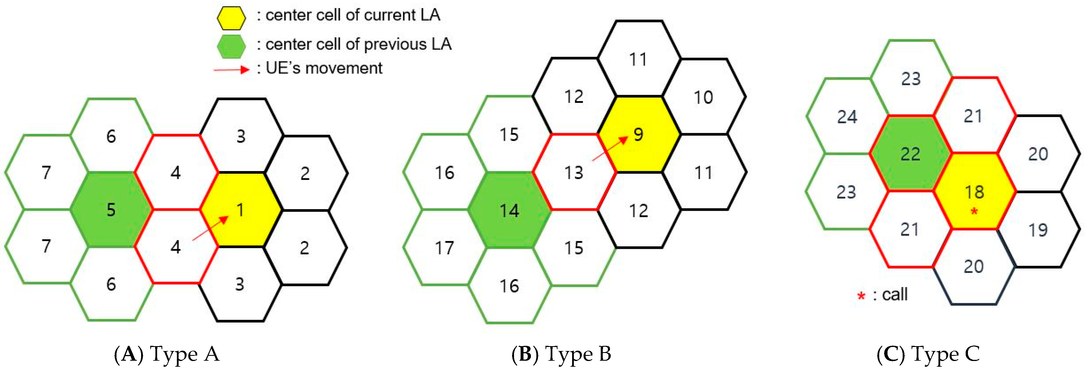
3.2.1. Three Types of Total LAs in 2D when D = 2
In the case of 2D when D = 2, total LAs (tLA) have three forms, as shown in Figure 2. Let us look at type A first. As shown in Figure 2A, type A indicates a case where a UE that has registered its location in a cell marked in green moves and registers its location in a yellow cell (which is one of the six closer cells out of the 12 cells surrounding ring 1-cells). In this case, LA1 (current LA) is defined as seven cells with a yellow cell as the center cell, and LA2 (previous LA) is defined as seven cells with a green cell as the center cell. In this case, the two middle cells are included in both Las.
Next, let us look at type B. Type B indicates a case where a UE that has registered its location in a green cell moves and registers its location in a yellow cell, which is farther away than the yellow cell of type A. Likewise, LA1 (current LA) is defined as seven cells with a yellow cell as the center cell, and LA2 (previous LA) is defined as seven cells with a green cell as the center cell. However, in the case of type B, only one cell in the middle overlaps with both LAs. Therefore, it has a different type of tLA from type A.
Next, let us look at type C. Type C refers to a case where a UE that has registered its location in a cell marked in green is moving and a call occurs in a yellow cell belonging to ring 1 of the current LA, resulting in implicit registration. In this case, LA1 (current LA) is defined as seven cells with a yellow cell as the center cell, and LA2 (previous LA) is defined as seven cells with a green cell as the center cell. In this case, the four middle cells are included in both LAs.
In Figure 2, numbers written in cells indicate states when applying the Markov chain model. Cells with the same stochastic properties are defined as being in the same state by writing the same numbers.
As a result, the tLA of the UE when D = 2 can be of three types, as shown in Figure 2 and Table 1. Location registration cost and paging cost must be calculated by analyzing which type the UE belongs to and which cell it belongs to.
Now, let us find the probability that the UE belongs to a specific cell (or state) in type A. Based on cell 1, where new location registration occurred, the states of the remaining cells in the tLA could be classified into states 2, 3, 4, 5, 6, and 7, as shown in Figure 2. State 5 and state 6 have the same distance from state 1, which is 2. However, state 5, unlike state 6, does not generate location registration even when moving to another cell. Thus, it must be classified differently from state 6. On the other hand, the two cells that make up state 6 have the same stochastic properties. Thus, they are classified as the same state.
Let us look at what other states the states defined in type A can transition to.
Through very sophisticated and time-consuming work, we can obtain a state transition diagram for all states. Since there are 25 states, the diagram is too large to be shown here. For readers’ understanding, the state transition diagram for some states related to type A is shown in Figure 3.
In Figure 3, state 1 indicates the state in which the cell has been entered and the final location registration has been performed. State 0 indicates that a call has occurred in the last location registered cell (state 1). From state 0 and state 1, transitions to state 0, state 2, state 3, and state 4 are possible. If a call occurs in state 1 (with probability 1 − m), the state becomes 0. Entering another cell in state 1 leads to states 2, 3, and 4, each with a probability of m/3. If another call occurs in state 0 (with probability 1 − m′), the state becomes 0 again. Entering another cell in state 0 leads to states 2, 3, and 4, each with a probability of m′/3.
If the UE enters another cell within the current tLA from state 2, it becomes states 1, 2, and 3 with a probability of m/6 for each. If it leaves the current tLA and enters a new cell, it becomes state 1 (with a probability of m/3) or state 9 (with a probability of m/6). It is worth noting that if a call occurs in state 2 (with a probability of 1 − m), the state becomes 18.
If the UE enters another cell within the current tLA from state 4, it will enter states 1, 3, 5, and 6 with a probability of m/6 for each. If it leaves the current tLA and enters a new cell, it will enter state 1 (with probability m/3). If a call occurs in state 4 (with probability 1 − m), the state becomes 0.
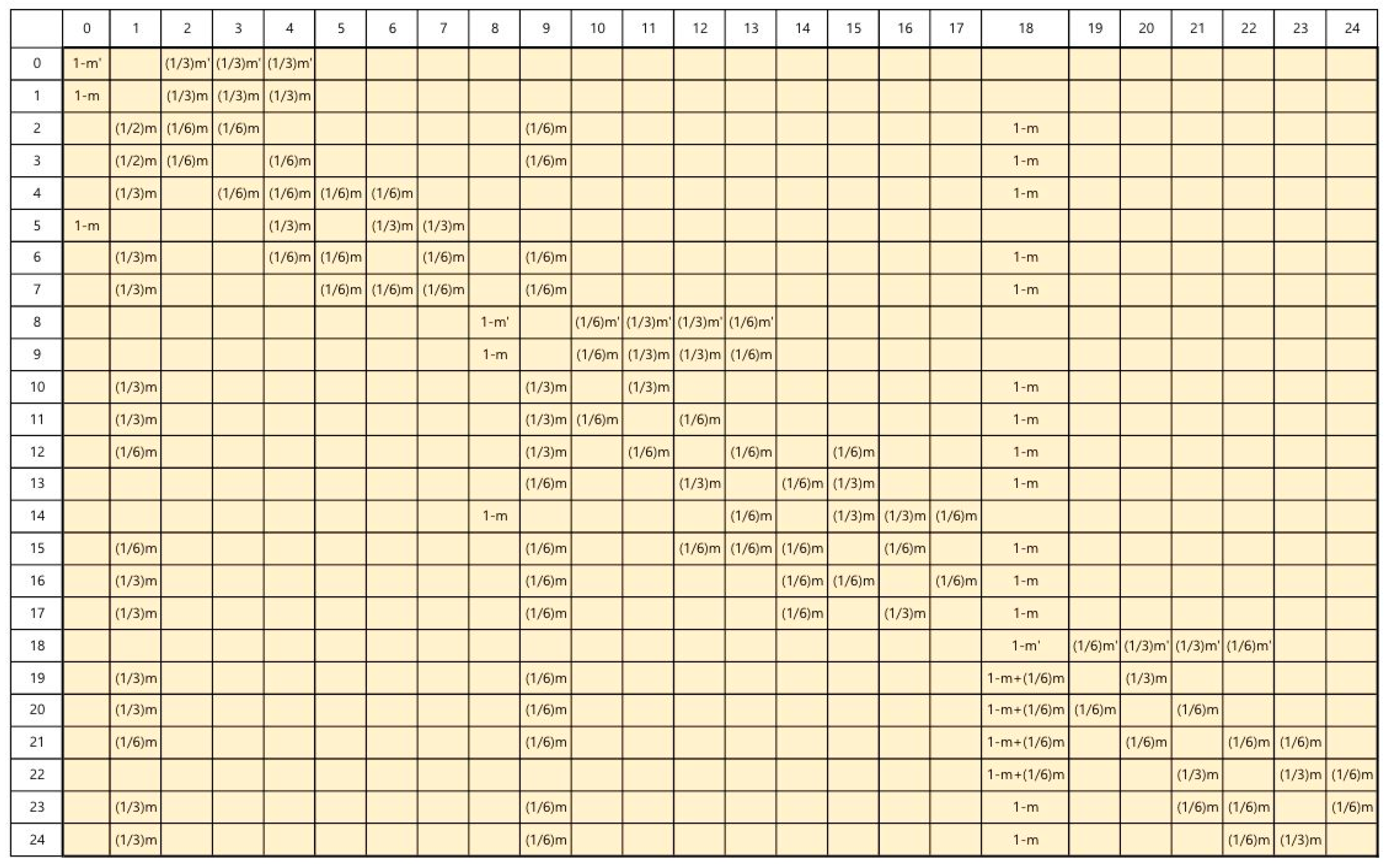
For states of type B and type C, the transition probability between states can be obtained through a similar process as type A. The final transition probability matrix P between a total of 25 states defined in these three types can be obtained as shown in Figure 4. State 0 indicates that a call has occurred in state 1 and state 8 indicates a state that a call has occurred in state 9. State 1 and state 9 become state 0 and state 8 when a call occurs. On the other hand, states 2, 3, 4, 6, and 7 become state 18 when a call occurs.
Therefore, the probability that the UE belongs to each type and the probability that the UE belongs to which cell of that type must be calculated. The location registration cost and paging cost must be derived by reflecting this.
3.2.2. Five Types of Total LAs in 2D when D = 3
The tLA of a UE when D = 3 is more complex than that when D = 2, although the approach is the same. Let us look at the tLA type of the UE when D = 3. In the case of 2D when D = 3, there are five types of tLA. Let us look at these in turn. The tLA of a UE when D = 3 is shown in Figure 5. According to the direction of movement in the edge cell, tLA, which is the union of the current LA and the previous LA, is defined differently, as shown in Figure 5A,B.
In addition, considering the implicit registration effect caused by the generation of a call, three types of tLA are possible. When a call occurs in a cell belonging to ring 1 in Figure 1, tLA is configured as shown in Figure 5C. Additionally, when a call occurs in one of the six farther cells out of the 12 cells in ring 2 in the current LA in Figure 1, the tLA is configured as shown in Figure 5D.
Lastly, when a call occurs in one of the six closer cells out of the 12 cells in ring 2 in the current LA in Figure 1, the tLA is configured as shown in Figure 5E.
As a result, the tLA of a UE when D = 3 is possible in five types, as shown in Figure 5 and Table 2. The location registration cost and paging cost must be calculated by analyzing which type the UE belongs to and which cell it belongs to.
Ultimately, in order to derive the optimal environment in 2D, the probability of the UE belonging to each type and the probability of the UE belonging to each state in that type must be calculated by varying the value of D. The location registration cost and paging cost must be derived by reflecting this.
First, let us find the probability that the UE belongs to a specific cell in type A. Based on cell 1, where a new location registration has occurred, the states of the remaining cells in the tLA can be classified into states 2 to 21, as shown in Figure 5. State 8 and state 9 have the same distance from state 1, which is 1. However, unlike state 9, state 8 must be classified differently from state 9 because the UE in state 8 can register its location after two cell entrances. On the other hand, the two cells that make up state 8 have the same stochastic properties. Thus, they are classified as the same state.
Let us look at what other states the states defined in type A can transition to. State 1 indicates the state in which the cell has been entered and the final location registration has been performed. State 0 indicates that a call has occurred in the last location-registered cell (state 1). From state 0 and state 1, transitions to states 0, 4, 6, 8, and 9 are possible. When entering another cell in state 1, it becomes states 4, 6, 8, and 9. Respective probabilities are m/6, m/3, m/3, and m/6. If a call occurs in state 1 with a probability of 1 − m, the state becomes 0. If another call occurs in state 0 with a probability of 1 − m′, the state becomes 0 again. When entering another cell, it becomes states 4, 6, 8, and 9 with probabilities of m′/6, m′/3, m′/3, and m′/6, respectively.
If the UE enters another cell within the current tLA from state 2, it will enter states 3 and 4 with probabilities of m/3 and m/6, respectively. If the UE leaves the current tLA and enters a new cell, it will enter state 1 (with a probability of m/3) or 23 (with a probability of m/6). It is worth noting that if a call occurs in state 2 (with probability 1 − m), the state becomes 70.
If the UE leaves the current tLA in state 10 and enters a new cell, it will enter states 1 and 23 with probabilities of m/6 and m/6, respectively. If the UE enters another cell within the current tLA, it becomes states 7, 8, 11, and 13 with a probability of m/6, respectively. If a call occurs in state 8 with a probability of 1 − m, the state becomes 55. If a call occurs in state 11 (with probability 1 − m), the state becomes 88.
For states of type B, C, D, and E, the transition probability between states can be obtained through a process similar to type A. A final transition probability matrix between a total of 104 states defined in these five types can be obtained. However, its size was too large to be included in the paper.
Finally, performance can be analyzed after obtaining the transition probability matrix for a total of 104 states defined in these five types. State 22 indicates a state in which a call has occurred in state 23. State 1 and state 23 become state 0 and state 22 when a call occurs. On the other hand, states 4, 6, 8, and 9 become state 55 when a call occurs, states 2, 5, 10, and 12 become state 70 when a call occurs, and states 3, 7, and 11 become state 88 when a call occurs.
Now, let us obtain the total signaling cost of 2D using a semi-Markov process model.
3.2.3. Calculation of State Transition Probabilities
In the state transition diagram, every transition probability contains m or m′. The first m is the probability that the UE entering a cell will move to the neighboring cell before a call occurs. m can be obtained as follows:
where is the Laplace–Stieltjes transform for .
Next, m′ is the probability that the UE, whose state has changed due to a call without entering a new cell, will move to the neighboring cell before another call occurs.
Rm is the interval between the arrival of the call and the time when the UE moves out of the cell. The probability density function of Rm, fr(t) comes from the random observer property [18]:
The Laplace–Stieltjes transform for the distribution is shown as follows:
Then, we have the following:
3.2.4. Calculation of Sojourn Time in Each State
It is necessary to note that the sojourn time in each state is different. For example, the sojourn time in state 1 is different from the sojourn time in state 0. The sojourn time in state 1 is the interval from the time a UE enters a cell until the time it leaves. On the other hand, the sojourn time in state 0 is the interval from the time a call occurs in a cell until the time it leaves.
In other words, if a UE entering a cell moves into a neighboring cell without a call occurring, then the sojourn time in the state is the interval from the time it enters a cell until the time it enters a neighboring cell. On the other hand, if a UE generates a call in a cell before it enters a neighboring cell, then the sojourn time in the state is the interval from the time it generates a call until the time it enters a neighboring cell.
It is necessary to consider that the sojourn time in each state is different to derive an accurate probability of the first paging failure.
Now, let us derive the sojourn time in state i (i = 1, 2, … 24 except 8 for D = 2, i = 1, 2, …, 103 except 22 for D = 3). The sojourn time in state i (i = 1, 2, … 24 except 8 for D = 2, i = 1, 2, …, 103 except 22 for D = 3) can be expressed as follows:
We can derive its mean as follows:
Next, let us derive the sojourn time in state j (j = 0, 8 for D = 2, and j = 0, 22 for D = 3). The sojourn time in state j (j = 0, 8 for D = 2, and j = 0, 22 for D = 3) can be expressed as follows:
Its mean can be derived as follows:
3.2.5. Calculation of Steady-State Probabilities
To obtain the steady-state probability considering different sojourn times, we first calculated the steady-state probability π for the usual Markov chain with transition probability P. This can be obtained using the following balanced equations [18]:
3.3. Registration Cost
By assuming that U is the registration cost of one registration, the registration cost per hour, Cu, can be obtained as follows:
where rk is the probability of location registration in state k when entering a neighboring cell.
3.4. Paging Cost
As described in Section 3.2, it is assumed that two-step paging is performed in 2D. The most recently registered LA is paged first. If there is no response, the remaining LA, except duplicated cells, is paged next. Assuming that V is the paging cost for one cell, the paging cost per hour, CP, can be obtained as follows:
where is the number of cells in an LA (=1 + 3D(D − 1)), and is the number of cells in total LA.
3.5. Total Signaling Cost
The final total signaling cost per hour can be obtained by adding the registration cost to the paging cost as follows:
4. Numerical Results
Let us compare the performances of 1D and 2D in various environments. First, for comparison in the same situation, it was assumed that the distance thresholds of the two methods were the same. Also, the following situation [4,5,6,7] is also assumed:
- Registration cost of one registration, U, is 10, and the paging cost for one cell, V, is 1 (U = 10, V = 1).
- Incoming and outgoing call rates are both one call per hour (λi = λo = 1).
- UE’s sojourn time in a cell, Tm, follows an exponential distribution with a mean of 1 (λm = 1).
To examine changes in mobility and call arrival characteristics, the call-to-mobility ratio (CMR) λi/λm is considered. For example, a CMR of 1/3 means a situation where the UE enters three cells during the incoming call arrival interval. As the CMR becomes smaller, the number of entering cells increases compared to the call arrival interval. In this study, three CMRs are assumed: 0.3, 0.4, and 0.5.
4.1. Registration Cost for 1D and 2D
Figure 6 shows the cost of location registration in 1D and 2D for various CMRs. From the figure, it can be seen that the location registration cost for 2D is significantly lower than that for 1D. Among the three cases shown in the figure, when looking at CMR = 0.3, where location registration occurs the most, compared to 1D, the location registration cost of 2D is decreased by 15.9%, 9.2%, or 1.5% when D = 1, 2, or 3, respectively. When looking at CMR = 0.5, where location registration occurs the least, compared to 1D, the location registration cost of 2D is decreased by 15.4%, 6.5%, or 0.8% when D = 1, 2, or 3, respectively.
It could be seen that there was no significant difference in the reduction rate according to the change in CMR. As the D value increased to 2 or 3, less location registration occurred in 2D than in 1D. However, the decrease rate was smaller than that when D = 1. It seemed that as the size of the LA increased, the frequent setup of new LAs due to the frequent occurrence of calls prior to location registrations increased, resulting in a reduction in regular location registrations in both 1D and 2D.
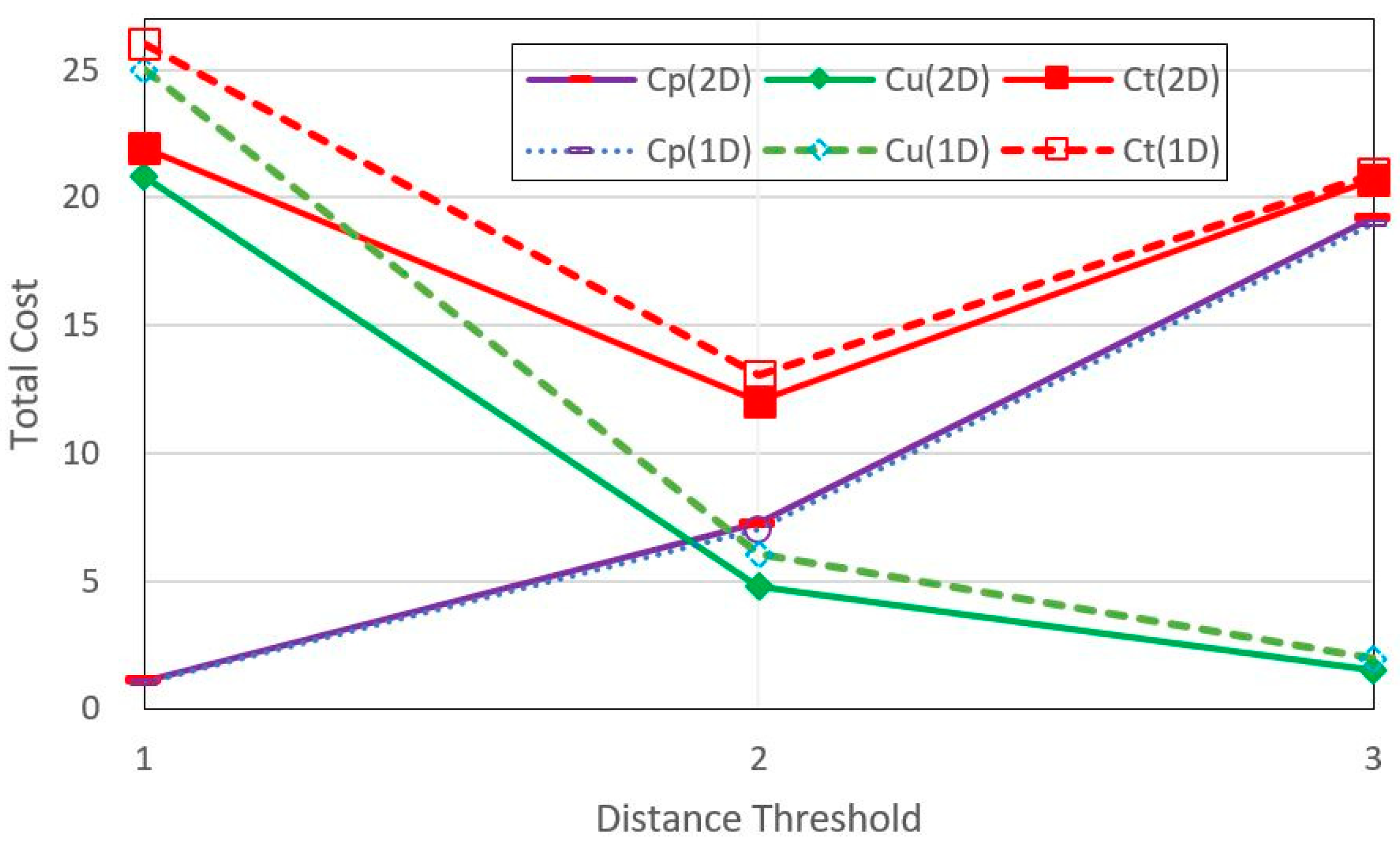
4.2. Total Cost for 1D and 2D
Figure 7 shows the total costs of 1D and 2D for CMR = 0.4. From the figure, we can see that 2D showed overall better performance than 1D in terms of total signaling cost. When CMR = 0.4 (entering 2.5 cells while one incoming call occurred), the total signaling cost for 2D decreased by 15.6%, 7.6%, or 1.0% when D = 1, 2, or 3, respectively, compared to 1D.
What was noteworthy in the figure was that as D increased to 1, 2, and 3, the location registration cost decreased rapidly, while the paging cost increased rapidly, reaching a minimum total signaling cost at D = 2. Another point to note in terms of comparing 1D and 2D was that while the location registration cost was significantly reduced in 2D compared to that in 1D, the reduction in paging cost was surprisingly small. The reason why paging costs did not increase significantly in 2D was that even if there were two LAs, the UE almost remained in the recently registered LA.
Since the actual mobile communication network will be operated in an environment where D = 2, where the total cost is the minimum, the actual reduction rate of the total signal cost of 2D can be said to be 7.6% in this environment.
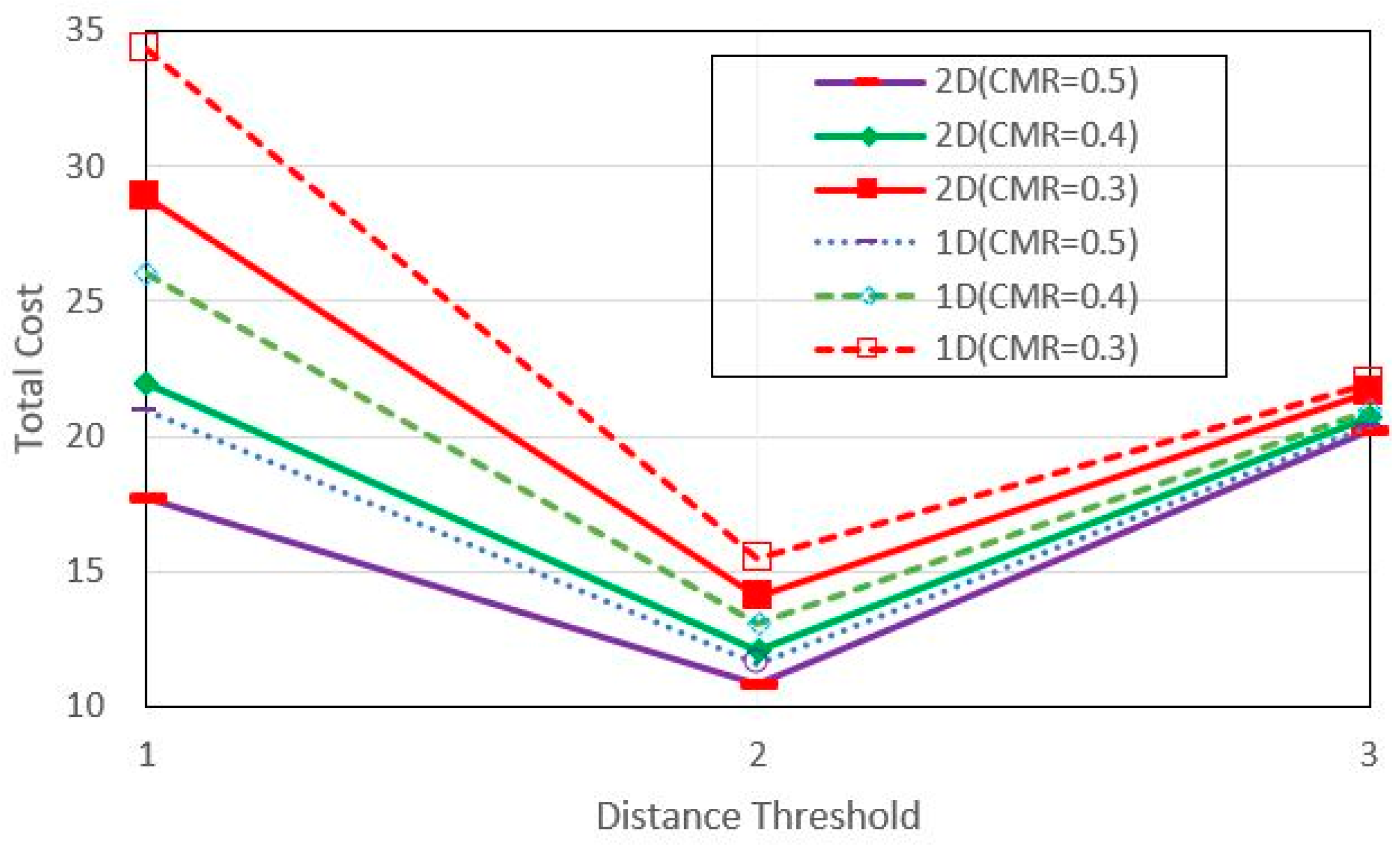
4.3. Total Cost for Various CMRs
Figure 8 shows the total cost for various CMRs. When CMR was 0.3, 0.4, or 0.5 at D = 2, where the total cost was minimum, the total cost of 2D was 9.2%, 7.6%, or 6.5% smaller than that at 1D, respectively, showing that 2D had a superior performance overall.
Looking at the figure, we could see that there was no significant difference in the total signaling cost of 1D and 2D in an environment where the CMR and distance threshold D were large (for example, when CMR = 0.5 and D = 3). This meant that as the CMR increased (i.e., as the number of cells the UE entered per call generation decreased), the number of location registrations decreased. Thus, the difference between the two methods was not large. In addition to a large CMR, if the distance threshold D also increased, the number of location registrations further decreased. Thus, the difference in location registration between 1D and 2D was bound to be subtle.
Additionally, as the D increased, the increase in paging cost, a disadvantage of 2D, tended to be more noticeable than the decrease in location registration cost, which was an advantage of 2D. In other words, as D increased, the number of cells in the LA increased, which meant that the paging cost increased. Therefore, in situations where the CMR was large and the D was also large, such as CMR = 0.5 and D = 3, the reduction in location registration cost might be minimal while the paging cost might increase rapidly. Thus, the total signaling costs of 1D and 2D might not be much different. In some cases, the total cost of 2D might be larger than that of 1D.
From the figure, it could be seen that even if the CMR changed, the value of D, which minimized total signaling costs of 1D and 2D in most environments, was 2. When comparing the performance at D = 2, where the total cost was minimal, 2D showed 6.5 to 9.2% better performance than 1D.
In conclusion, it can be seen that 2D outperforms 1D in most actual mobile communication environments. However, since 2D is not better than 1D in all cases, it is necessary to select an appropriate location registration method by comprehensively considering the system environment, adaptability to expansion, and operational convenience.
4.4. Effect of Implicit Registration by Outgoing Calls
As explained before, when an outgoing call from the UE is made in a cell, the network updates the location through the call processing messages without the registration process, which is called an implicit registration by an outgoing call. Therefore, as the number of outgoing calls increases, the location registration cost will decrease. Furthermore, in this case, the paging cost can be reduced in 2D since the network can update the UE’s current cell.
Figure 9 compares the performance results of 1D and 2D for various outgoing call rates, assuming the incoming call rate is 1. In the figure, λo = i means that the outgoing call rate is i. From the figure, we can see that 2D with a high outgoing call rate is superior to 1D with the same rate.
In this instance, 1 − [2D(λo = 1)/2D(λo = i)] means the reduction ratio of 2D when the outgoing call rate increases by i. From the figure, we can see that, when D = 2, 2D with λo = 3 reduces the cost by 13% compared to 2D with λo = 1.
Note that, when D = 2, 2D with a low outgoing call rate (λo = 1) is sometimes inferior to 1D with a high outgoing call rate (λo = 3). In conclusion, the implicit registration effect by outgoing calls should be considered to minimize the total cost.
4.5. Total Signaling Cost for Various Gamma Distributions
Let us consider the case where the UE’s sojourn time in a cell, Tm, follows a gamma distribution with a mean of 0.4. We will focus on the variances in gamma distributions.
Assuming E(Tm) = 0.4, Figure 10 compares performance results for various variances of Tm. The figure showed that, as the variance increased, 2D was much more superior to 1D. In order to increase the variance while maintaining the same mean in the gamma distribution, the shape parameter must be decreased. In this case, the probability that the sojourn time in the cell was less than the mean increase, which made the location registration increase, thus reducing the total signaling cost in 2D more significantly with an advantage from the viewpoint of location registration than in 1D.
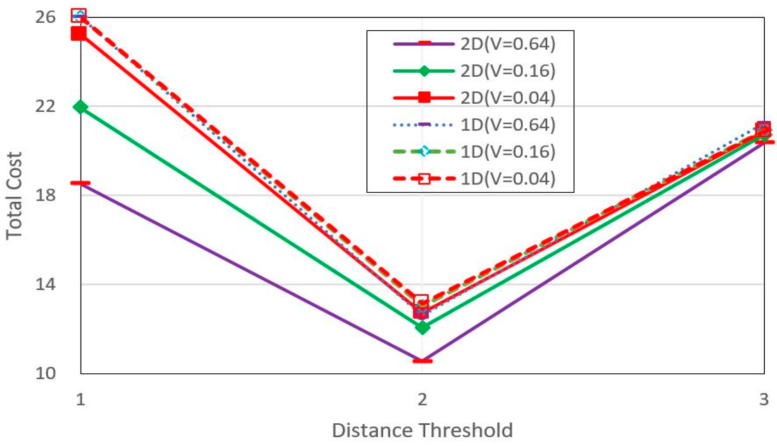
4.6. Total Cost for Simultaneous Paging
Let us consider the case when simultaneous paging is applied to both 1D and 2D. Figure 11 shows that, in this environment (CMR = 0.4), 1D is much more superior to 2D at D = 2 where the total cost is minimal. Through many numerical results for various CMRs, it could be seen that, when simultaneous paging was applied to both 1D and 2D, 1D was superior to 2D in most cases, unless the CMR was very small.
However, in the figure, 2D was superior to 1D at D = 1. If DBR in which LA increased on a cell-by-cell basis [7] was introduced, 2D might be superior to 1D between D = 1 and D = 2. Thus, a more sophisticated analysis is needed.
Since better performance between 1D and 2D will vary depending on the various situations, optimal performance can be achieved by reflecting the network environment in real time and dynamically changing to operate in the method that provides better performance among the two methods.
5. Conclusions
In order to provide mobile communication services to more subscribers within limited radio channels, the efficiency of radio channels must be increased. Achieving this goal calls for the implementation of an efficient location registration method. Two typical location registration methods applicable to the actual mobile communication network are zone-based registration (ZBR) and distance-based registration (DBR).
This study focused on DBR where new location registration occurs only after moving a minimum distance D from the point where the previous location registration occurred. Unlike ZBR, DBR generates the location registration cost equally across all cells in the mobile communication network. Furthermore, DBR allows dynamic location registration by varying the distance threshold for each UE depending on the characteristics of the UE, and the performance can be improved by leveraging the implicit registration effects of outgoing calls.
To improve the performance of DBR with one LA (1D), DBR with two LAs (2D) was proposed. In 2D, location registration becomes unnecessary when crossing two stored LAs. But this is at the cost of relatively higher paging costs than the existing 1D method. Whether to use one method or the other depends on the balance between the reduced costs of location registration and the increased costs of paging.
An accurate mathematical model for 2D has been lacking. In this study, we presented an accurate mathematical model to analyze the performance of 2D for the first time. A semi-Markov process model was used, assuming a two-dimensional random walk mobility model in a hexagonal cell environment. Unlike 1D, it was difficult to analyze the performance of 2D since total location areas (tLA) could have various forms. The 2D method was modeled as a comprehensive Markov chain with three types of tLA (25 states) for D = 2 and five types of tLA (105 states) for D = 3. Location registration costs and paging costs were calculated using a semi-Markov process model to analyze the UE’s type and cell association.
Our proposed mathematical model accurately evaluated performance showing that 2D with two-step paging is better than existing 1D in all but a few cases. Nonetheless, 2D does not always outperform 1D. Thus, when choosing a location registration method, one should take into consideration factors such as system environment, suitability for system expansion, and operational convenience. The results of this study can serve to guide the selection and implementation of an appropriate location management method depending on the environment in which the network operates.
It is important to note that this study only presents a conceptual idea of constructing two LAs in DBR, and implementing the proposed method in contemporary mobile networks poses challenges. Future studies will examine implementation possibilities, taking into account hierarchical cell layouts, the possibility of two-step paging, and internetworking with mobile peer-to-peer networks [19,20].
Funding
This work was supported by grants from the National Research Foundation (NRF) funded by the Ministry of Science and ICT (No. 2022R1F1A1074141), .
Institutional Review Board Statement
Not applicable.
Informed Consent Statement
Not applicable.
Data Availability Statement
Data are contained within the article.
Conflicts of Interest
The author has no conflicts of interest relevant to this study to disclose.
References
- 3GPP2 C.S0005-F v2.0, Upper Layer (Layer 3) Signaling Standard for cdma2000 Spread Spectrum Systems. May 2014. Available online: https://www.arib.or.jp/english/html/overview/doc/STD-T64v6_80/Specification/ARIB_STD-T64-C.S0005-Fv2.0.pdf (accessed on 1 May 2023.).
- Lin, Y.B. Reducing location update cost in a PCS network. IEEE/ACM Trans. Netw. 1997, 5, 25–33. [Google Scholar]
- Jung, J.; Baek, J.H. Analyzing Zone-Based Registration Using a Three Zone System: A Semi-Markov Process Approach. Appl. Sci. 2020, 10, 5705. [Google Scholar] [CrossRef]
- Baek, J.H. Improvement and performance evaluation when implementing a distance-based registration. Appl. Sci. 2021, 11, 6823. [Google Scholar] [CrossRef]
- Zhu, Y.-h.; Leung, V.C.M. Optimization of Distance-Based Location Management for PCS Networks. IEEE Trans. Wirel. Comm. 2008, 7, 3507–3516. [Google Scholar] [CrossRef]
- Baek, J.H.; Lee, T.H.; Kim, C.S. Performance analysis of 2-location distance-based registration in mobile communication networks. IEICE Trans. Commun. 2013, E96-B, 914–917. [Google Scholar] [CrossRef]
- Li, K. Analysis of Distance-Based Location Management in Wireless Communication Networks. IEEE Trans. Parallel Distrib. Syst. 2013, 24, 225–238. [Google Scholar] [CrossRef]
- Mao, Z.; Douligeris, C. A location-based mobility tracking scheme for PCS networks. Comput. Commun. 2000, 23, 1729–1739. [Google Scholar] [CrossRef]
- Li, K. Location distribution of a mobile terminal and its application to paging cost reduction and minimization. J. Parallel Distrib. Comput. 2017, 99, 68–89. [Google Scholar] [CrossRef]
- Wang, X.; Lei, X.; Fan, P.; Hu, R.; Horng, S. Cost analysis of movement-based location management in PCS networks: An embedded Markov chain approach. IEEE Trans. Veh. Technol. 2014, 63, 1886–1902. [Google Scholar] [CrossRef]
- Liu, P.; Liu, Y.; Ge, L.; Chen, C. An Embedded Markov Chain Modeling Method for Movement-Based Location Update Scheme. J. Commun. 2015, 10, 512–519. [Google Scholar] [CrossRef]
- Alhashimi, H.F.; Hindia, M.N.; Dimyati, K.; Hanafi, E.B.; Safie, N.; Qamar, F.; Azrin, K.; Nguyen, Q.N. A Survey on Resource Management for 6G Heterogeneous Networks: Current Research, Future Trends, and Challenges. Electronics 2023, 12, 647. [Google Scholar] [CrossRef]
- Mukhtar, M.; Yunus, F.; Alqahtani, A.; Arif, M.; Brezulianu, A.; Geman, O. The Challenges and Compatibility of Mobility Management Solutions for Future Networks. Appl. Sci. 2022, 12, 11605. [Google Scholar] [CrossRef]
- Alsaeedy, A.A.R.; Chong, E.K.P. Tracking area update and paging in 5G networks: A survey of problems and solutions. Mob. Netw. Appl. 2019, 24, 578–595. [Google Scholar] [CrossRef]
- Banafaa, M.; Shayea, I.; Din, J.; Azmi, M.H.; Alashbi, A.; Daradkeh, Y.I.; Alhammadi, A. 6G mobile communication technology: Requirements, targets, applications, challenges, advantages, and opportunities. Alex. Eng. J. 2023, 64, 245–274. [Google Scholar] [CrossRef]
- Siddiqui, M.U.A.; Qamar, F.; Tayyab, M.; Hindia, M.N.; Nguyen, Q.N.; Hassan, R. Mobility management issues and solutions in 5G-and-beyond network: A comprehensive review. Electronics 2022, 11, 1366. [Google Scholar] [CrossRef]
- Gures, E.; Shayea, I.; Alhammadi, A.; Ergem, M. A comprehensive survey on mobility management in 5G heterogeneous networks: Architectures, challenges and solutions. IEEE Access 2020, 8, 195883–195913. [Google Scholar] [CrossRef]
- Ross, S. Introduction to Probability Models, 11th ed.; Elsevier: Cambridge, MA, USA, 2014. [Google Scholar]
- Arunachalam, A.; Ravi, V.; Krichen, M.; Alroobaea, R.; Alqurni, J.-S. Analytical Comparison of Resource Search Algorithms in Non-DHT Mobile Peer-to-Peer Networks. Comput. Mater. Contin. 2021, 68, 983–1001. [Google Scholar] [CrossRef]
- Seddiki, M.; Benchaïba, M. SWS: A Smart Walk mechanism for resources search in unstructured mobile P2P networks. In Proceedings of the 2015 First International Conference on New Technologies of Information and Communication (NTIC), Mila, Algeria, 8–9 November 2015; pp. 1–6. [Google Scholar] [CrossRef]
Figure 1.
Location areas for distance-based registration (D = 3).

Figure 2.
Three types of total LAs in 2D when D = 2.

Figure 3.
State transition diagram for some states in 2D (D = 2).

Figure 4.
Transition probability matrix P for 2D when D = 2.

Figure 5.
Five types of total LAs in 2D when D = 3.

Figure 6.
Registration cost for various CMRs.

Figure 7.
Total cost for CMR = 0.4.

Figure 8.
Total cost for various CMRs.

Figure 9.
Effect of implicit registration by outgoing calls (CMR = 0.4).

Figure 10.
Total cost for various gamma distributions (CMR = 0.4).

Figure 11.
Total cost for simultaneous paging (CMR = 0.4).


Table 1.
Three types of total LAs of 2D when D = 2.
| Type | Conditions for Entry into This Type | No. of Cells in tLA (No. of Overlapping Cells in Both LAs) | No. of States in Markov Chain Model |
|---|---|---|---|
| A | The UE enters one of the 6 closer cells out of the 12 cells surrounding ring 1 cells in current LA. | 12 (2) | 8 (=7 + 1) |
| B | The UE currently enters one of the 6 farther cells out of the 12 cells surrounding ring 1 cells in current LA. | 13 (1) | 10 (=9 + 1) |
| C | A call occurs in a cell in ring 1. | 10 (4) | 7 |
Table 2.
Five types of total LAs of 2D when D = 3.
| Type | Conditions for Entry into This Type | No. of Cells in tLA (No. of Overlapping Cells in Both LAs) | No. of States in Markov Chain Model |
|---|---|---|---|
| A | The UE enters one of the 6 farther cells out of the 18 cells surrounding ring 2 cells in current LA. | 34 (4) | 22 (=21 + 1) |
| B | The UE enters one of the 12 closer cells out of the 18 cells surrounding ring 2 cells in current LA. | 32 (6) | 33 (=32 + 1) |
| C | A call occurs in a cell in ring 1. | 24 (14) | 16 |
| D | A call occurs in one of the 6 farther cells out of the 12 cells in ring 2 in current LA. | 29 (9) | 15 |
| E | A call occurs in one of the 6 closer cells out of the 12 cells in ring 2 in current LA. | 28 (10) | 18 |
Disclaimer/Publisher’s Note: The statements, opinions and data contained in all publications are solely those of the individual author(s) and contributor(s) and not of MDPI and/or the editor(s). MDPI and/or the editor(s) disclaim responsibility for any injury to people or property resulting from any ideas, methods, instructions or products referred to in the content. |
© 2024 by the author. Licensee MDPI, Basel, Switzerland. This article is an open access article distributed under the terms and conditions of the Creative Commons Attribution (CC BY) license (https://creativecommons.org/licenses/by/4.0/).
Share and Cite
MDPI and ACS Style
Baek, J.-H. Analyzing Distance-Based Registration with Two Location Areas: A Semi-Markov Process Approach. Electronics 2024, 13, 233. https://doi.org/10.3390/electronics13010233
AMA Style
Baek J-H. Analyzing Distance-Based Registration with Two Location Areas: A Semi-Markov Process Approach. Electronics. 2024; 13(1):233. https://doi.org/10.3390/electronics13010233
Chicago/Turabian StyleBaek, Jang-Hyun. 2024. "Analyzing Distance-Based Registration with Two Location Areas: A Semi-Markov Process Approach" Electronics 13, no. 1: 233. https://doi.org/10.3390/electronics13010233
Note that from the first issue of 2016, this journal uses article numbers instead of page numbers. See further details here.