
A Simple Learning Approach for Robust Tracking Control of a Class of Dynamical Systems


Abstract
:1. Introduction
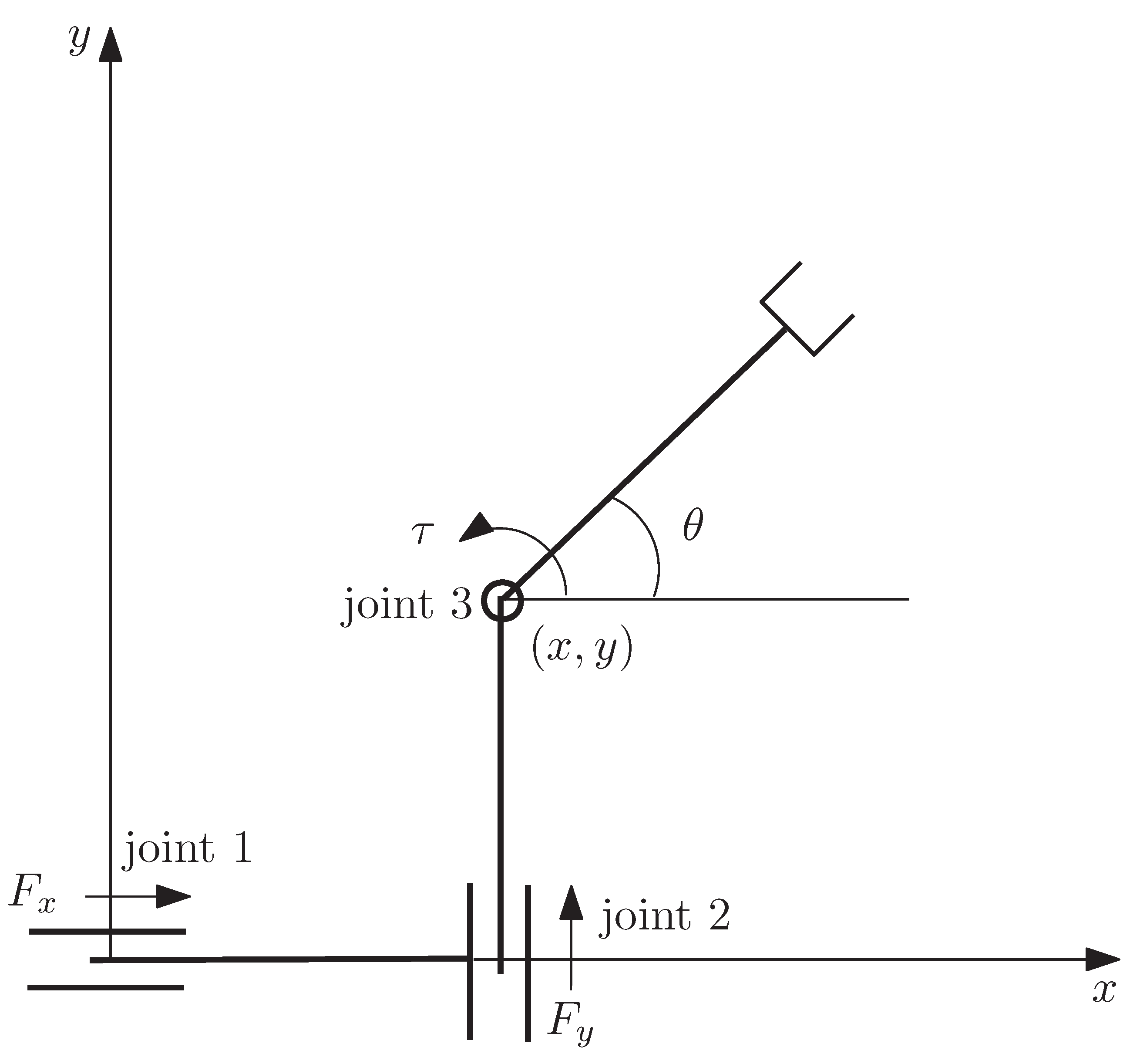
2. Mathematical Model
3. Control Design
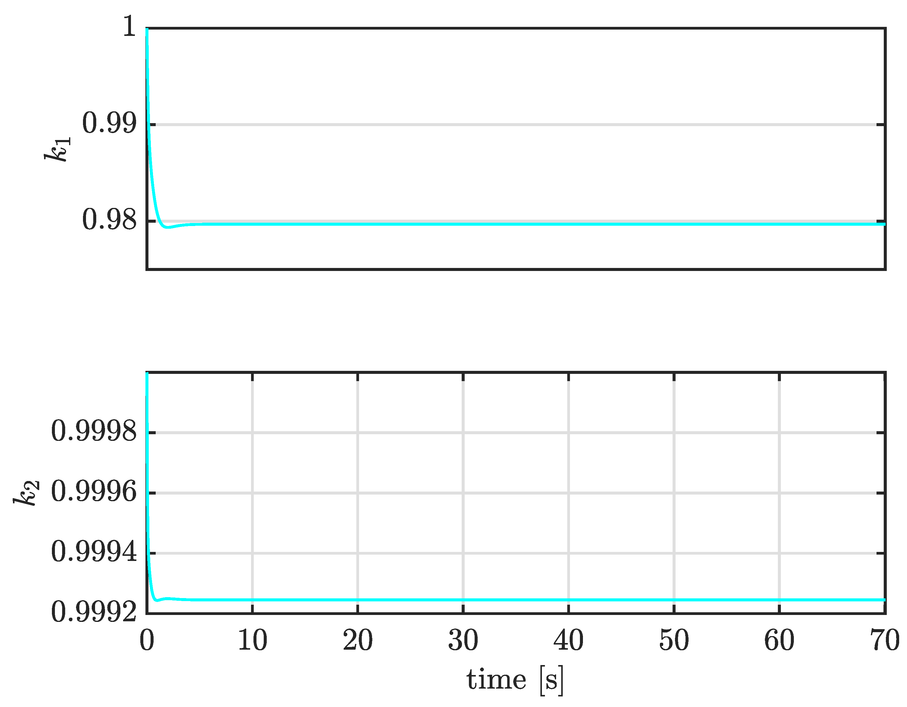
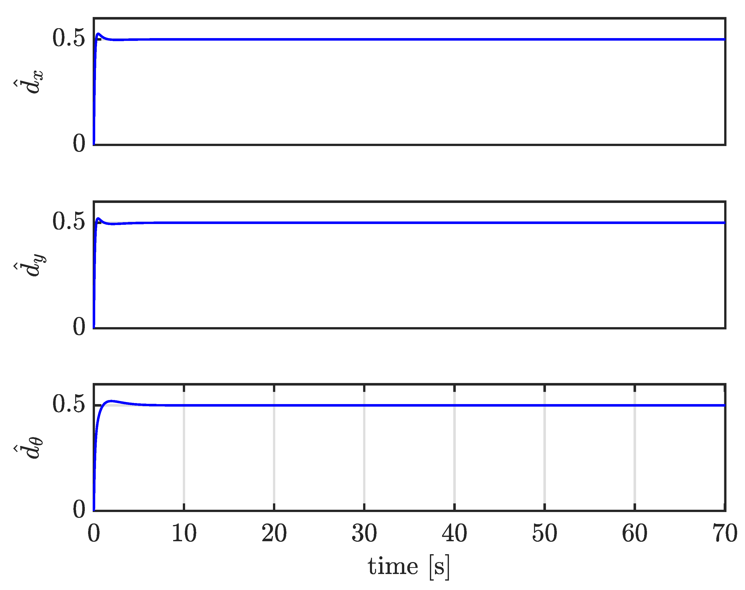
3.1. Update Rules
3.2. Stability Proof
4. Example: Simple Learning Control of a PPR Robot
4.1. Computer Simulation Results
- Case I: Tracking sinusoidal trajectories;
- Case II: Tracking constant trajectories;
- Case III: Tracking under large external disturbances.
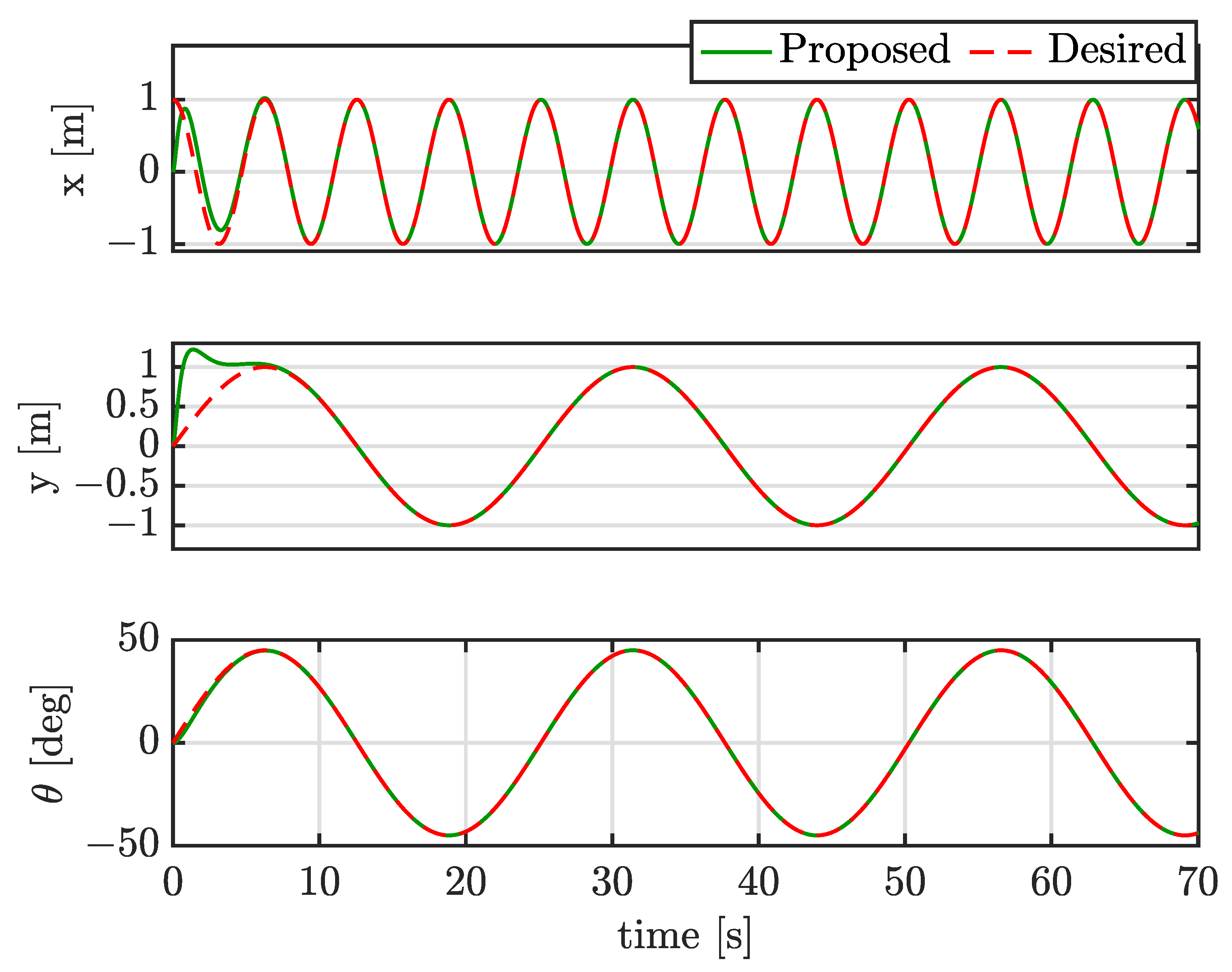
4.2. Case I: Tracking Sinusoidal Trajectories
4.3. Case II: Tracking Constant Trajectories
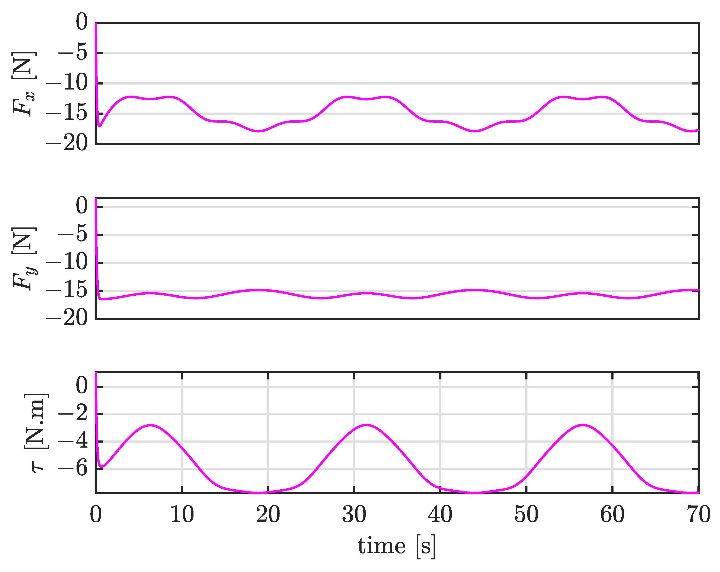
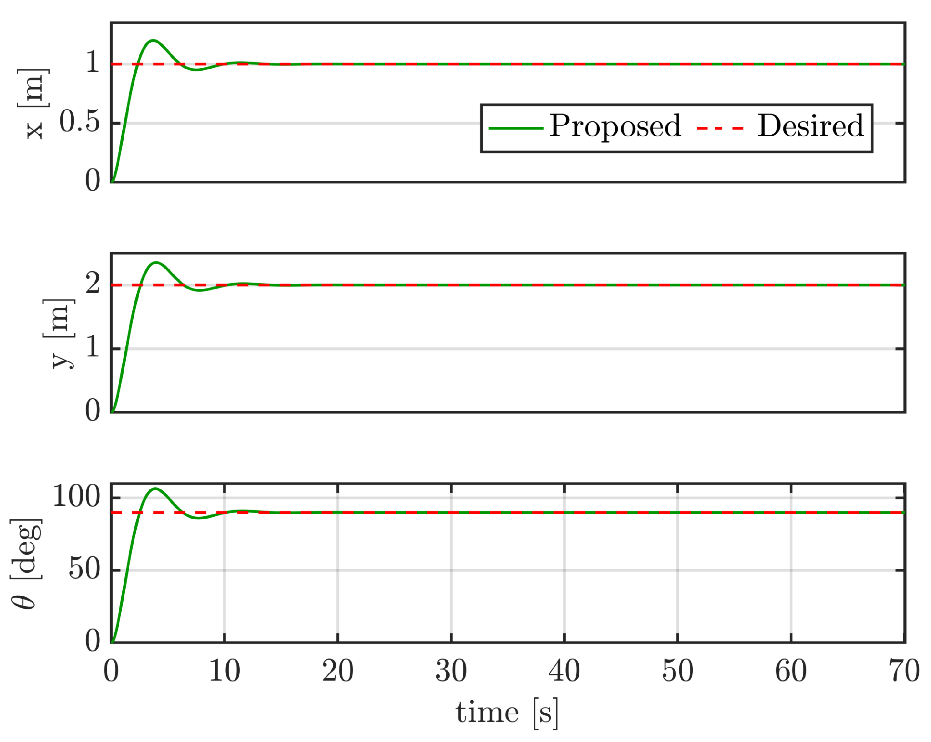
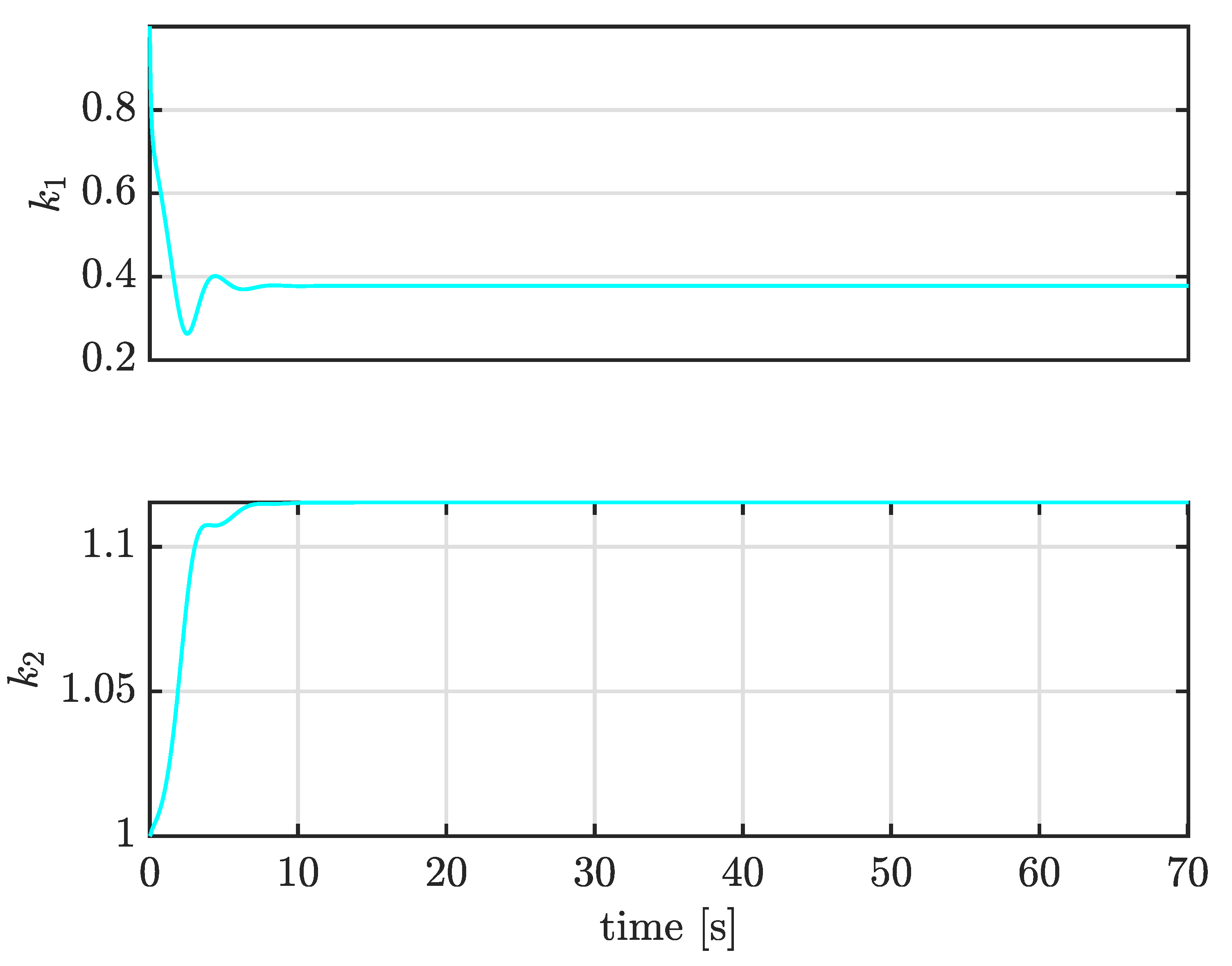
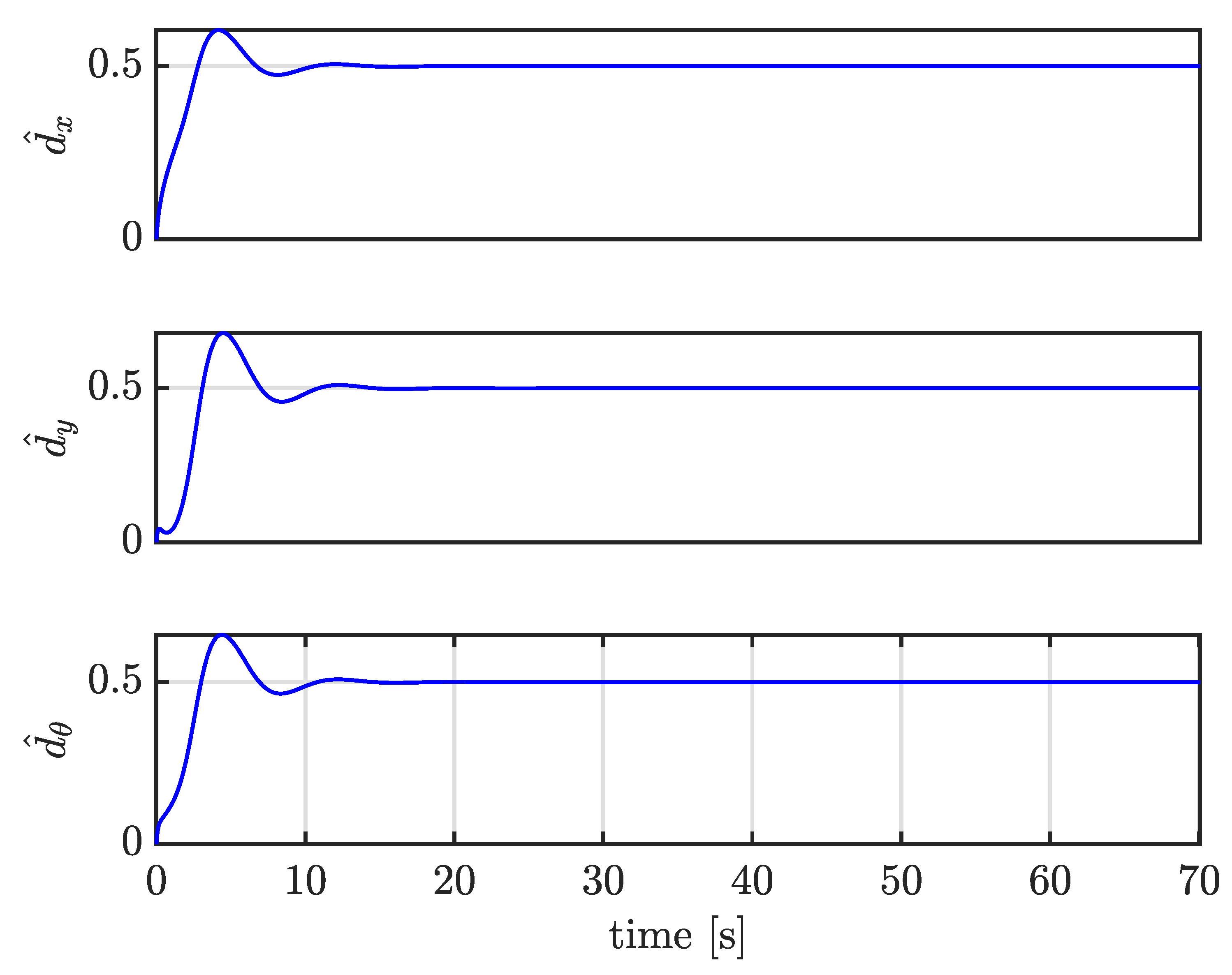
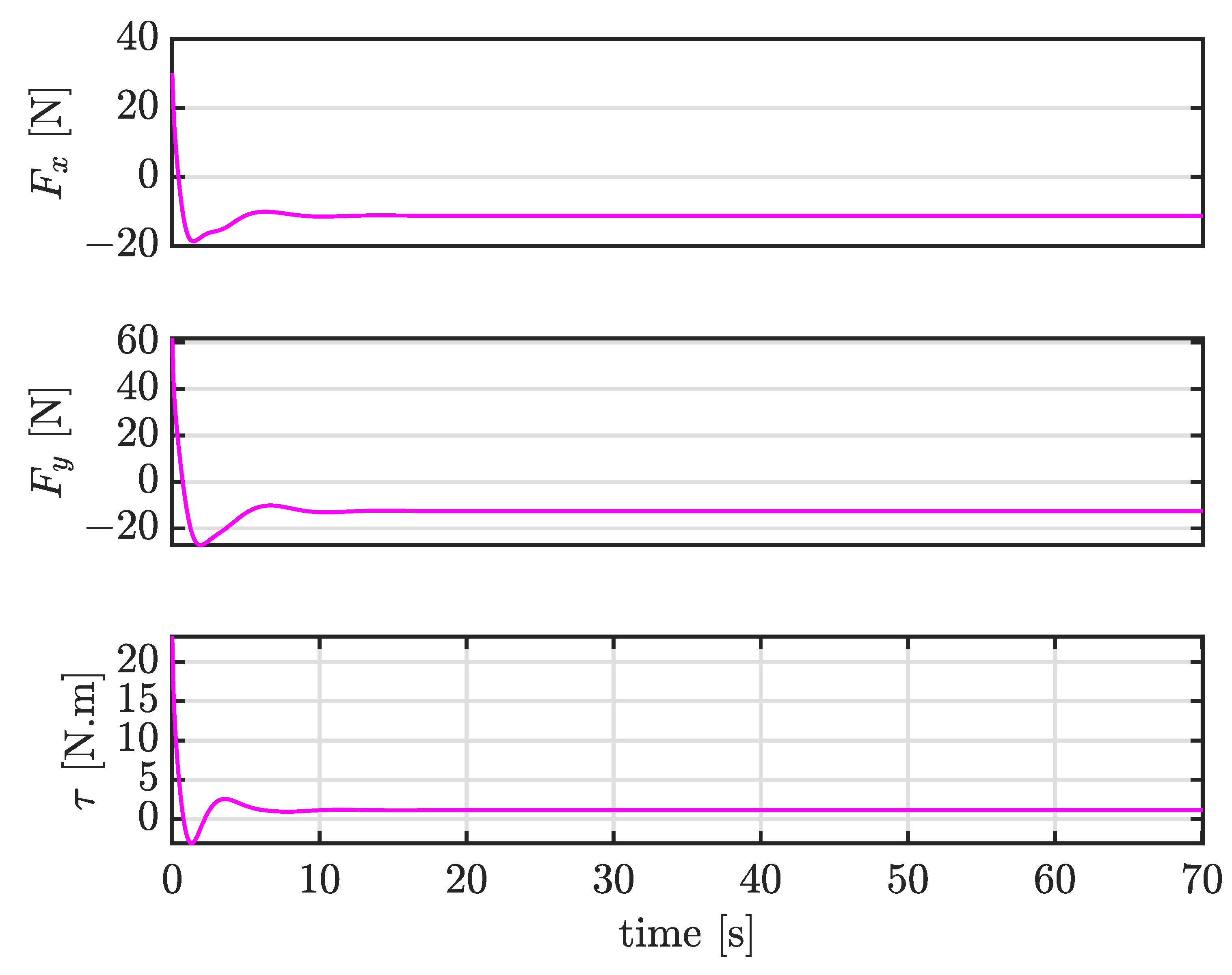
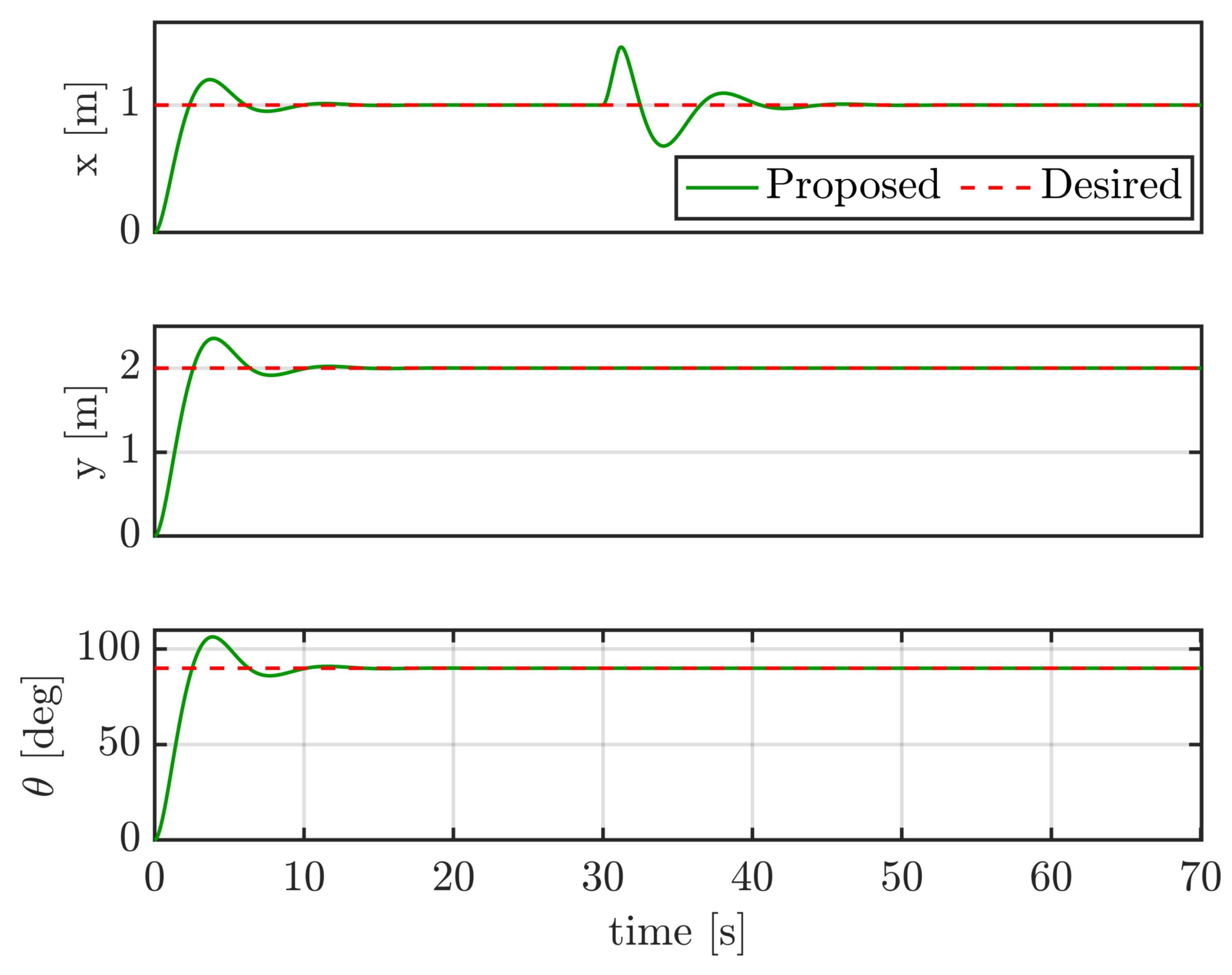
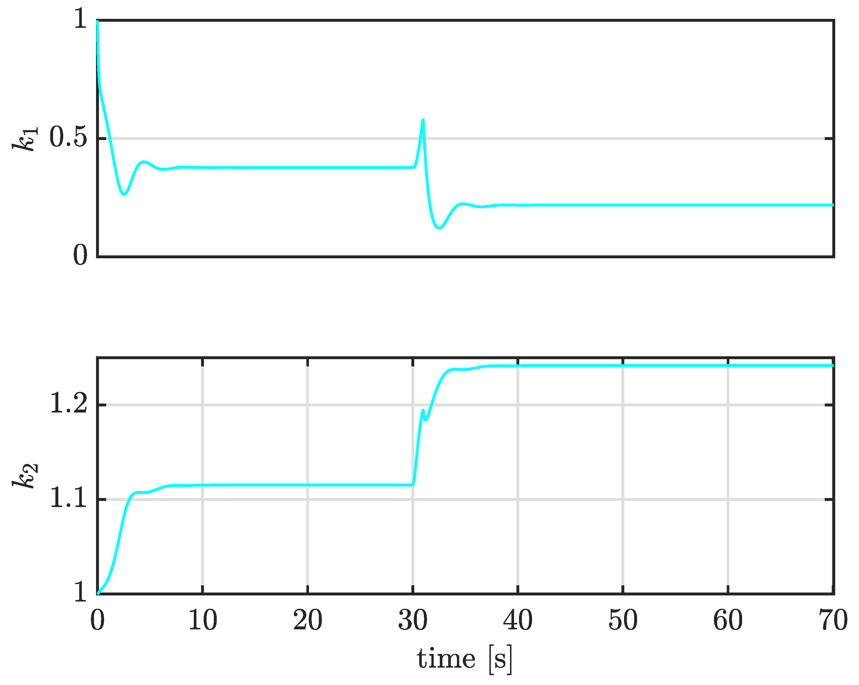
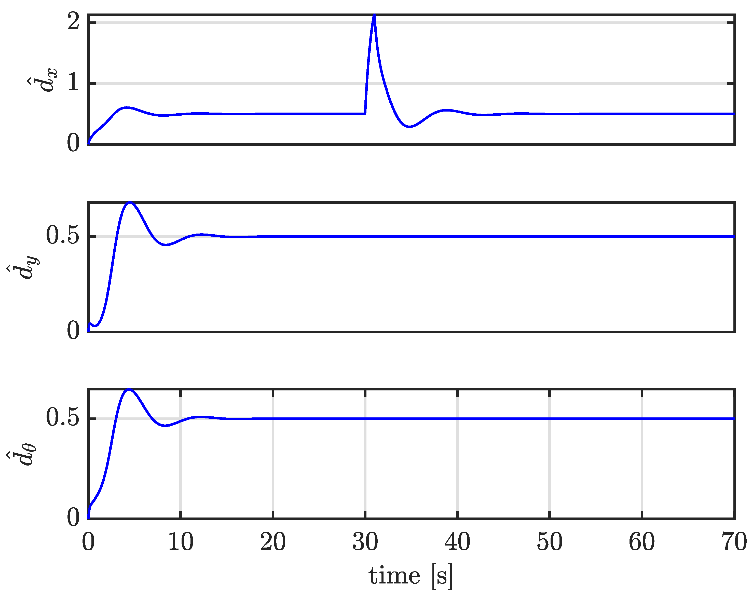
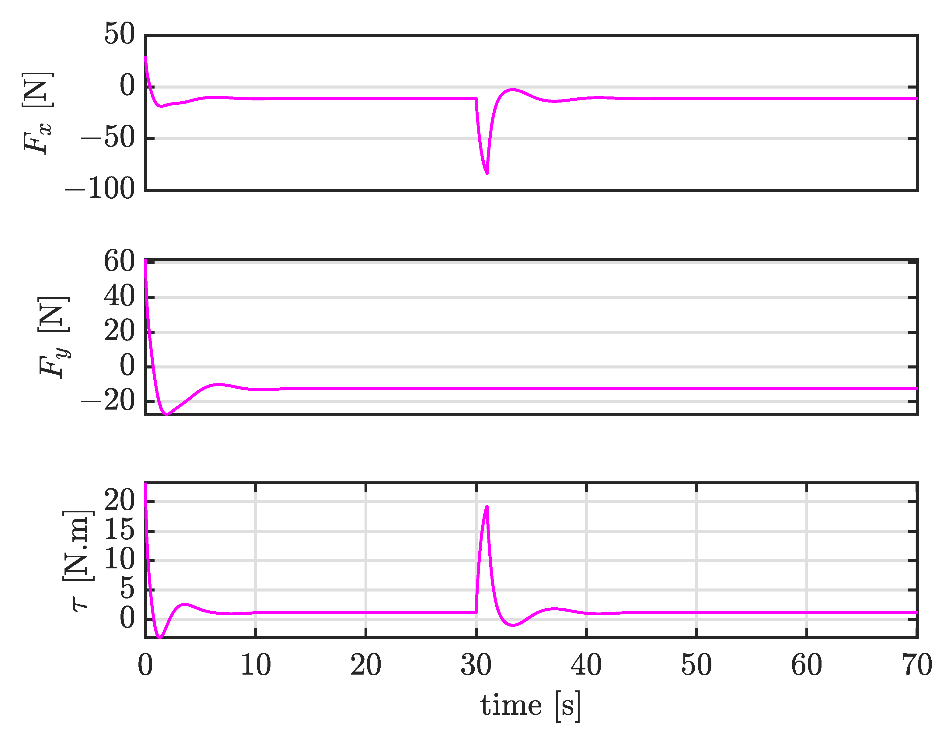
4.4. Case III: Trajectory Tracking under Large External Disturbances
5. Conclusions
Author Contributions
Funding
Data Availability Statement
Acknowledgments
Conflicts of Interest
References
- Izaguirre-Espinosa, C.; Muñoz-Vázquez, A.J.; Sanchez-Orta, A.; Parra-Vega, V.; Castillo, P. Contact force tracking of quadrotors based on robust attitude control. Control. Eng. Pract. 2018, 78, 89–96. [Google Scholar] [CrossRef]
- Mammarella, M.; Capello, E.; Park, H.; Guglieri, G.; Romano, M. Tube-based robust model predictive control for spacecraft proximity operations in the presence of persistent disturbance. Aerosp. Sci. Technol. 2018, 77, 585–594. [Google Scholar] [CrossRef]
- Ambati, P.R.; Padhi, R. Robust auto-landing of fixed-wing UAVs using neuro-adaptive design. Control Eng. Pract. 2017, 60, 218–232. [Google Scholar] [CrossRef]
- Muniraj, D.; C, P.M.; Guthrie, K.T.; Farhood, M. Path-following control of small fixed-wing unmanned aircraft systems with H∞ type performance. Control Eng. Pract. 2017, 67, 76–91. [Google Scholar] [CrossRef]
- Zhao, B.; Xian, B.; Zhang, Y.; Zhang, X. Nonlinear robust adaptive tracking control of a quadrotor UAV via immersion and invariance methodology. IEEE Trans. Ind. Electron. 2015, 62, 2891–2902. [Google Scholar] [CrossRef]
- Mystkowski, A. Implementation and investigation of a robust control algorithm for an unmanned micro-aerial vehicle. Robot. Auton. Syst. 2014, 62, 1187–1196. [Google Scholar] [CrossRef]
- Liu, H.; Bai, Y.; Lu, G.; Zhong, Y. Robust attitude control of uncertain quadrotors. IET Control Theory Appl. 2013, 7, 1583–1589. [Google Scholar] [CrossRef]
- Roy, S.; Baldi, S.; Fridman, L.M. On adaptive sliding mode control without a priori bounded uncertainty. Automatica 2020, 111, 108650. [Google Scholar] [CrossRef]
- Kayacan, E. Sliding mode learning control of uncertain nonlinear systems with Lyapunov stability analysis. Trans. Inst. Meas. Control 2019, 41, 1750–1760. [Google Scholar] [CrossRef]
- Liu, Z.; Liu, X.; Chen, J.; Fang, C. Altitude control for variable load quadrotor via learning rate based robust sliding mode controller. IEEE Access 2019, 7, 9736–9744. [Google Scholar] [CrossRef]
- Babaei, A.R.; Malekzadeh, M.; Madhkhan, D. Adaptive super-twisting sliding mode control of 6-DOF nonlinear and uncertain air vehicle. Aerosp. Sci. Technol. 2019, 84, 361–374. [Google Scholar] [CrossRef]
- Liu, L.; Zhu, J.; Tang, G.; Bao, W. Diving guidance via feedback linearization and sliding mode control. Aerosp. Sci. Technol. 2015, 41, 16–23. [Google Scholar] [CrossRef]
- Ramirez-Rodriguez, H.; Parra-Vega, V.; Sanchez-Orta, A.; Garcia-Salazar, O. Robust backstepping control based on integral sliding modes for tracking of quadrotors. J. Intell. Robot. Syst. 2014, 73, 51–66. [Google Scholar] [CrossRef]
- Kayacan, E. Sliding mode control for systems with mismatched time-varying uncertainties via a self-learning disturbance observer. Trans. Inst. Meas. Control 2019, 41, 2039–2052. [Google Scholar] [CrossRef]
- Kayacan, E.; Saeys, W.; Ramon, H.; Belta, C.; Peschel, J. Experimental validation of linear and nonlinear MPC on an articulated unmanned ground vehicle. IEEE/ASME Trans. Mechatronics 2018, 23, 2023–2030. [Google Scholar] [CrossRef]
- Ostafew, C.J.; Schoellig, A.P.; Barfoot, T.D. Robust constrained learning-based NMPC enabling reliable mobile robot path tracking. Int. J. Robot. Res. 2016, 35, 1547–1563. [Google Scholar] [CrossRef]
- Kayacan, E.; Kayacan, E.; Ramon, H.; Saeys, W. Learning in centralized nonlinear model predictive control: Application to an autonomous tractor-trailer system. IEEE Trans. Control Syst. Technol. 2015, 23, 197–205. [Google Scholar] [CrossRef]
- Mehndiratta, M.; Kayacan, E.; Patel, S.; Kayacan, E.; Chowdhary, G. Learning-based fast nonlinear model predictive control for custom-made 3D printed ground and aerial robots. In Handbook of Model Predictive Control; Birkhäuser: Cham, Switzerland, 2019; pp. 581–605. [Google Scholar]
- Kocer, B.B.; Tjahjowidodo, T.; Seet, G.G.L. Centralized predictive ceiling interaction control of quadrotor VTOL UAV. Aerosp. Sci. Technol. 2018, 76, 455–465. [Google Scholar] [CrossRef]
- Dierks, T.; Jagannathan, S. Output feedback control of a quadrotor UAV using neural networks. IEEE Trans. Neural Netw. 2010, 21, 50–66. [Google Scholar] [CrossRef]
- Nicol, C.; Macnab, C.J.B.; Ramirez-Serrano, A. Robust neural network control of a quadrotor helicopter. In Proceedings of the 2008 Canadian Conference on Electrical and Computer Engineering, Niagara Falls, ON, Canada, 4–7 May 2008; pp. 1233–1238. [Google Scholar]
- Fu, C.; Hong, W.; Zhang, L.; Guo, X.; Tian, Y. Adaptive robust backstepping attitude control for a multi-rotor unmanned aerial vehicle with time-varying output constraints. Aerosp. Sci. Technol. 2018, 78, 593–603. [Google Scholar] [CrossRef]
- Wu, B.; Wu, J.; He, W.; Tang, G.; Zhao, Z. Adaptive neural control for an uncertain 2-DOF helicopter system with unknown control direction and actuator faults. Mathematics 2022, 10, 4342. [Google Scholar] [CrossRef]
- Jafari, M.; Marquez, G.; Selberg, J.; Jia, M.; Dechiraju, H.; Pansodtee, P.; Teodorescu, M.; Rolandi, M.; Gomez, M. Feedback control of bioelectronic devices using machine learning. IEEE Control Syst. Lett. 2020, 5, 1133–1138. [Google Scholar] [CrossRef]
- Zhu, G.; Wu, X.; Yan, Q.; Cai, J. Robust learning control for tank gun control servo systems under alignment condition. IEEE Access 2019, 7, 145524–145531. [Google Scholar] [CrossRef]
- Xu, Z.; Li, W.; Wang, Y. Robust learning control for shipborne manipulator with fuzzy neural network. Front. Neurorobotics 2019, 13, 11. [Google Scholar] [CrossRef] [PubMed]
- Kayacan, E.; Khanesar, M.A.; Rubio-Hervas, J.; Reyhanoglu, M. Learning control of fixed-wing unmanned aerial vehicles using fuzzy neural networks. Int. J. Aerosp. Eng. 2017, 2017, 5402809. [Google Scholar] [CrossRef]
- Wu, S.; Wen, S.; Liu, Y.; Zhang, K. Robust adaptive learning control for spacecraft autonomous proximity maneuver. Int. J. Pattern Recognit. Artif. Intell. 2017, 31, 1759007. [Google Scholar] [CrossRef]
- Imanberdiyev, N.; Kayacan, E. A fast learning control strategy for unmanned aerial manipulators. J. Intell. Robot. Syst. 2019, 94, 805–824. [Google Scholar] [CrossRef]
- Kayacan, E.; Kayacan, E.; Khanesar, M.A. Identification of nonlinear dynamic systems using Type-2 fuzzy neural networks—A novel learning algorithm and a comparative study. IEEE Trans. Ind. Electron. 2015, 62, 1716–1724. [Google Scholar] [CrossRef]
- Khanesar, M.A.; Kayacan, E.; Reyhanoglu, M.; Kaynak, O. Feedback error learning control of magnetic satellites using type-2 fuzzy neural networks with elliptic membership functions. IEEE Trans. Cybern. 2015, 45, 858–868. [Google Scholar] [CrossRef]
- Han, H.G.; Yang, F.F.; Yang, H.Y.; Wu, X.L. Type-2 fuzzy broad learning controller for wastewater treatment process. Neurocomputing 2021, 459, 188–200. [Google Scholar] [CrossRef]
- Kayacan, E.; Kayacan, E.; Ramon, H.; Saeys, W. Adaptive neuro-fuzzy control of a spherical rolling robot using sliding-mode-control-theory-based online learning algorithm. IEEE Trans. Cybern. 2013, 43, 170–179. [Google Scholar] [CrossRef] [PubMed]
- Rossomando, F.G.; Soria, C.; Carelli, R. Sliding mode neuro adaptive control in trajectory tracking for mobile robots. J. Intell. Robot. Syst. 2014, 74, 931–944. [Google Scholar] [CrossRef]
- Topalov, A.V.; Kaynak, O. Online learning in adaptive neurocontrol schemes with a sliding mode algorithm. IEEE Trans. Syst. Man Cybern. Part B Cybern. 2001, 31, 445–450. [Google Scholar] [CrossRef] [PubMed]
- Kayacan, E.; Fossen, T.I. Feedback linearization control for systems with mismatched uncertainties via disturbance observers. Asian J. Control 2019, 21, 1064–1076. [Google Scholar] [CrossRef]
- de Jesús Rubio, J. Robust feedback linearization for nonlinear processes control. ISA Trans. 2018, 74, 155–164. [Google Scholar] [CrossRef]
- Jafari, M.; Xu, H.; Garcia Carrillo, L.R. A neurobiologically-inspired intelligent trajectory tracking control for unmanned aircraft systems with uncertain system dynamics and disturbance. Trans. Inst. Meas. Control 2019, 41, 417–432. [Google Scholar] [CrossRef]
- Jafari, M.; Xu, H. Intelligent control for unmanned aerial systems with system uncertainties and disturbances using artificial neural network. Drones 2018, 2, 30. [Google Scholar] [CrossRef]
- Şahin, S. Learning feedback linearization using artificial neural networks. Neural Process. Lett. 2016, 44, 625–637. [Google Scholar] [CrossRef]
- Umlauft, J.; Beckers, T.; Kimmel, M.; Hirche, S. Feedback linearization using Gaussian processes. In Proceedings of the 2017 IEEE 56th Annual Conference on Decision and Control (CDC), Melbourne, Australia, 12–15 December 2017; pp. 5249–5255. [Google Scholar]
- Hou, Z.; Jin, S. Model Free Adaptive Control: Theory and Applications; CRC Press: Boca Raton, FL, USA, 2013. [Google Scholar]
- Chi, R.; Hou, Z.; Huang, B.; Jin, S. A unified data-driven design framework of optimality-based generalized iterative learning control. Comput. Chem. Eng. 2015, 77, 10–23. [Google Scholar] [CrossRef]
- Zhu, Y.; Hou, Z. Data-driven MFAC for a class of discrete-time nonlinear systems with RBFNN. IEEE Trans. Neural Netw. Learn. Syst. 2014, 25, 1013–1020. [Google Scholar] [CrossRef]
- Hou, Z.; Zhu, Y. Controller-dynamic-linearization-based model free adaptive control for discrete-time nonlinear systems. IEEE Trans. Ind. Inform. 2013, 9, 2301–2309. [Google Scholar] [CrossRef]
- Hou, Z.; Chi, R.; Gao, H. An overview of dynamic-linearization-based data-driven control and applications. IEEE Trans. Ind. Electron. 2017, 64, 4076–4090. [Google Scholar] [CrossRef]
- Liu, H.; Zhao, W.; Zuo, Z.; Zhong, Y. Robust control for quadrotors with multiple time-varying uncertainties and delays. IEEE Trans. Ind. Electron. 2017, 64, 1303–1312. [Google Scholar] [CrossRef]
- Meda-Campaña, J.A. On the estimation and control of nonlinear systems with parametric uncertainties and noisy outputs. IEEE Access 2018, 6, 31968–31973. [Google Scholar] [CrossRef]
- You, S.; Son, Y.S.; Gui, Y.; Kim, W. Gradient-descent-based learning gain for backstepping controller and disturbance observer of nonlinear systems. IEEE Access 2023, 11, 2743–2753. [Google Scholar] [CrossRef]
- Chen, W.H.; Yang, J.; Guo, L.; Li, S. Disturbance-observer-based control and related methods: An overview. IEEE Trans. Ind. Electron. 2016, 63, 1083–1095. [Google Scholar] [CrossRef]
- Huang, J.; Ri, S.; Liu, L.; Wang, Y.; Kim, J.; Pak, G. Nonlinear disturbance observer-based dynamic surface control of mobile wheeled inverted pendulum. IEEE Trans. Control. Syst. Technol. 2015, 23, 2400–2407. [Google Scholar] [CrossRef]
- Kayacan, E.; Peschel, J.M.; Chowdhary, G. A self-learning disturbance observer for nonlinear systems in feedback-error learning scheme. Eng. Appl. Artif. Intell. 2017, 62, 276–285. [Google Scholar] [CrossRef]
- Chen, W.H. Disturbance observer based control for nonlinear systems. IEEE/ASME Trans. Mechatron. 2004, 9, 706–710. [Google Scholar] [CrossRef]
- Dutta, L.; Das, D.K. Nonlinear disturbance observer based adaptive explicit nonlinear model predictive control design for a class of nonlinear MIMO system. IEEE Trans. Aerosp. Electron. Syst. 2023, 59, 1965–1979. [Google Scholar] [CrossRef]
- Ren, B.; Zhong, Q.C.; Dai, J. Asymptotic reference tracking and disturbance rejection of UDE-based robust control. IEEE Trans. Ind. Electron. 2017, 64, 3166–3176. [Google Scholar] [CrossRef]
- Mehndiratta, M.; Kayacan, E.; Reyhanoglu, M.; Kayacan, E. Robust tracking control of aerial robots via a simple learning strategy-based feedback linearization. IEEE Access 2019, 8, 1653–1669. [Google Scholar] [CrossRef]
- Reyhanoglu, M.; Jafari, M.; Rehan, M. Simple learning-based robust trajectory tracking control of a 2-DOF helicopter system. Electronics 2022, 11, 2075. [Google Scholar] [CrossRef]
- Goldstein, H.; Poole, C.; Safko, J. Classical Mechanics; Addison Wesley: San Francisco, CA, USA, 2002. [Google Scholar]
- Langson, W.; Alleyne, A. A stability result with application to nonlinear regulation: Theory and experiments. In Proceedings of the 1999 American Control Conference (Cat. No. 99CH36251), San Diego, CA, USA, 2–4 June 1999; Volume 5, pp. 3051–3056. [Google Scholar]
- Reyhanoglu, M.; van der Schaft, A.; McClamroch, N.H.; Kolmanovsky, I. Dynamics and control of a class of underactuated mechanical systems. IEEE Trans. Autom. Control 1999, 44, 1663–1671. [Google Scholar] [CrossRef]


| Symbol | Parameter | Value | Unit |
|---|---|---|---|
| Link 1 mass | 5 | kg | |
| Link 2 mass | 10 | kg | |
| Link 3 mass | 15 | kg | |
| MOI of link 3 about its CoM | 1.5 | kg·m | |
| l | Distance b/w revolute joint and CoM of link 3 | m |
| Symbol | Parameter | Value | Unit |
|---|---|---|---|
| Link 1 mass | 4 | kg | |
| Link 2 mass | 8 | kg | |
| Link 3 mass | 12 | kg | |
| MOI of link 3 about its CoM | 1.7 | kg·m | |
| l | Distance b/w revolute joint and CoM of link 3 | m |
Disclaimer/Publisher’s Note: The statements, opinions and data contained in all publications are solely those of the individual author(s) and contributor(s) and not of MDPI and/or the editor(s). MDPI and/or the editor(s) disclaim responsibility for any injury to people or property resulting from any ideas, methods, instructions or products referred to in the content. |
© 2023 by the authors. Licensee MDPI, Basel, Switzerland. This article is an open access article distributed under the terms and conditions of the Creative Commons Attribution (CC BY) license (https://creativecommons.org/licenses/by/4.0/).
Share and Cite
Reyhanoglu, M.; Jafari, M. A Simple Learning Approach for Robust Tracking Control of a Class of Dynamical Systems. Electronics 2023, 12, 2026. https://doi.org/10.3390/electronics12092026
Reyhanoglu M, Jafari M. A Simple Learning Approach for Robust Tracking Control of a Class of Dynamical Systems. Electronics. 2023; 12(9):2026. https://doi.org/10.3390/electronics12092026
Chicago/Turabian StyleReyhanoglu, Mahmut, and Mohammad Jafari. 2023. "A Simple Learning Approach for Robust Tracking Control of a Class of Dynamical Systems" Electronics 12, no. 9: 2026. https://doi.org/10.3390/electronics12092026