1. Introduction
The power systems of today are large, highly interconnected mechanisms with electrical and mechanical components that are significantly affected by every social or natural event. In their early construction, they were designed according to some specifications. (1) Power flow was designed to be from generation to distribution, through the transmission. (2) Loads of cities and industries with their demand characteristics for a specific time period were easily forecasted and they were generally known to the power system operator. (3) The power was generated in bulk power stations such as large thermal plants, hydro-power plants, and nuclear plants and transmitted to the customers. Aside from their carbon footprints or harm to nature, the generation of a power system was fully controllable and the generated power was matched easily to the demand. Therefore, a quasi-steady-state operation was achieved for a large power system. Additionally, the monitoring and control of most of the system were designed according to the steady-state operation of the system [
1].
Coming from the past to our present day, none of the above assumptions hold. We see distributed energy resources (DERs) at every level of the system. Factories and households are covering their rooftops with solar panels, and there are wind and solar farms with variable sizes and capacities depending on their location of installment. With the high penetration of renewables and storage systems, the generation also is now harder to predict and control, as it depends on many parameters. Furthermore, consumers evolving into the concept of prosumers reduce their energy demand by generating a portion of their need, and even they sell the excess amount to the system after complying with the grid requirements. They are now controlling their demand according to the electricity price at that moment, using their renewables and battery storage systems. All these new developments in the demand side made load forecasting harder. As a result, matching the supply with demand became a difficult task for power system operators. Along with the installment of renewables to both industry and households, the number of unpredictable events such as pandemics and lockdowns has increased and that puts the power system under stress furthermore since these new developments push the system to operate far away from the quasi-steady-state operation. Therefore, the dynamic behavior of the power system has gained more importance than ever. To be able to know the response of a power system with a nonlinear behavior to a dynamic event requires intense computation power and accurate modeling of the components of the system. Power system operators of today have the required computation power and are able to simulate these events before they happen, but the modeling of the system is cumbersome. The simulations of the operation were normal before the 10 August 1996 blackout in western America. However, the system did not reach stability after a dynamic event, and a complete blackout occurred, affecting the electricity use of 7.49 million customers in western North America [
2]. Aftermath studies of the blackout indicated that simulation parameters of the power plants were different from their real-life values. Therefore the Western Systems Coordinating Council (WSCC) put regular calibrations of plant parameters into practice.
Formerly, the calibration process of plant parameters was performed offline, being costly and inefficient since the power plant is taken out of the grid (no generation and selling to the market) during the tests, and the tests are labor-intensive to the generation company. With the advancements in sensors and computation power throughout the system, some online calibration tools that can be great alternatives to offline staged tests have been proposed in recent years. The use of phasor measurement units (PMUs) with their GPS-synchronized measurements enables these online calibration methods to be performed sufficiently accurately [
3]. More and more system states become observable to the power system operator, which unlocks the state estimation procedures with the increased amount of measurement data. There is a variety of studies conducted on the improvement of dynamic state estimation.
The identification of problematic parameters of a power plant can be performed by comparing the voltage magnitude, angle, and active/reactive power outputs of the plant at the point of interconnection. Since the data refresh rate of PMUs is higher than the conventional SCADA measurements, these devices can accurately capture the dynamic behavior of the plant during a transient event. In [
4], problematic parameters are identified via trajectory sensitivity analysis, and identified parameters are calibrated by comparing the Hilbert spectrum of problematic parameters and model output curves. In [
5], an iterative deep-learning-based framework is proposed for parameter calibration, using the PMU measurements in the event playback during the training of the model.
Least squares-based approaches are commonly used in state and parameter estimation. In [
6], the frequency response of the power system against the generation losses is estimated. The inertia constant of the power system and the total online capacity of spinning-reserve support generators are estimated via the measurements of transient frequency changes during a dynamic event. The least-squares method is used to estimate the coefficients of polynomial curve fitting. Another study in [
7] focuses on estimating the uncertainty of parameters with a Bayesian approach. Inertia parameters of three synchronous generators in an IEEE-9 bus system are estimated. In [
8], the parameter estimation of WECC composite load models under fault conditions is performed with a nonlinear least-squares (NLS) approach, where the simulated and measured outputs are compared and the fitting error is minimized. The method is improved by feeding the priori information on parameter values to the model. In [
9], an adaptive parameter estimation for generator inertia is performed, using the modal frequency and damping measurements. Based on the weighted-least-squares (WLS) method, the sensitivities of the modal frequency and damping measurements to the parameters, are utilized.
Besides least-squares-estimation (LSE) methods, another class for online state and parameter estimation is Kalman-filter-based approaches. In [
10], a
extended Kalman filter for the estimation of dynamic states is implemented to limit the influence of model uncertainties in the dynamic model representation of the system. In [
11], a constrained iterated unscented Kalman filter is performed to estimate the dynamic states and unknown parameters of two-axis modeled generators, with arbitrary initialization and large errors presented to the parameters. The filter is proven to be robust against these conditions. Another example of this class is the ensemble Kalman filter which is used in [
12] to estimate erroneous parameters and achieve an accurate dynamic model for the stability analysis of the system. It is a sequential Monte Carlo implementation of the general Bayesian recursive filter. The ensemble Kalman filter (EnKF) utilizes an ensemble of samples to represent and propagate the probability density function (PDF) of the state variable vector
x [
12]. The parameters to be calibrated are also considered as states and included in the variable vector
x. To increase the performance of the filter, preliminary procedures such as sanity check and trajectory sensitivity analysis are performed. With the increase in computation power and measurement data via PMUs, the calibration process can be performed, and hence the calibrated simulation models will provide more reliable decision support for the system operator.
This paper is the extended version of the conference paper in [
13] where the parameters of the simulation model of conventional synchronous generators are calibrated with an ensemble Kalman filter. Before the calibration of parameters, preliminary sensitivity and collinearity analyses are performed to eliminate the unidentifiable parameters, as suggested in [
14], where the proposed EnKF method is implemented on conventional synchronous generators with the WSCC9 bus system as a working case. Implementation is performed in the Python
TM environment using the API functions of SIEMENS PSS®E software (v35.5). In this paper, the synchronous generator is replaced with a Type 4 wind turbine generator, and the rest of the working case is kept the same. In addition to the work conducted in [
13], two more parameters of the wind turbine generator are calibrated as can be seen in the simulation results section. Furthermore, non-converging behavior in Type 4 wind turbine generators for some parameters, is observed in this paper. The reasons for this behavior and its possible solution methods are discussed in
Section 5. Detection of convergence criteria for the parameter calibration is mentioned at the end of the paper, further research will be carried out on this issue as a milestone in the way of turning the proposed method into a calibration tool that is generalized for most of the simulation models.
The rest of the paper is organized as follows. In
Section 2 the preliminary procedures of event playback, sensitivity, and collinearity analysis and the employed ensemble Kalman filter algorithm are explained. In
Section 3, the implementation environment and the conditions of the calibration are explained. In
Section 4, the results of the employed method are presented.
3. Implementation
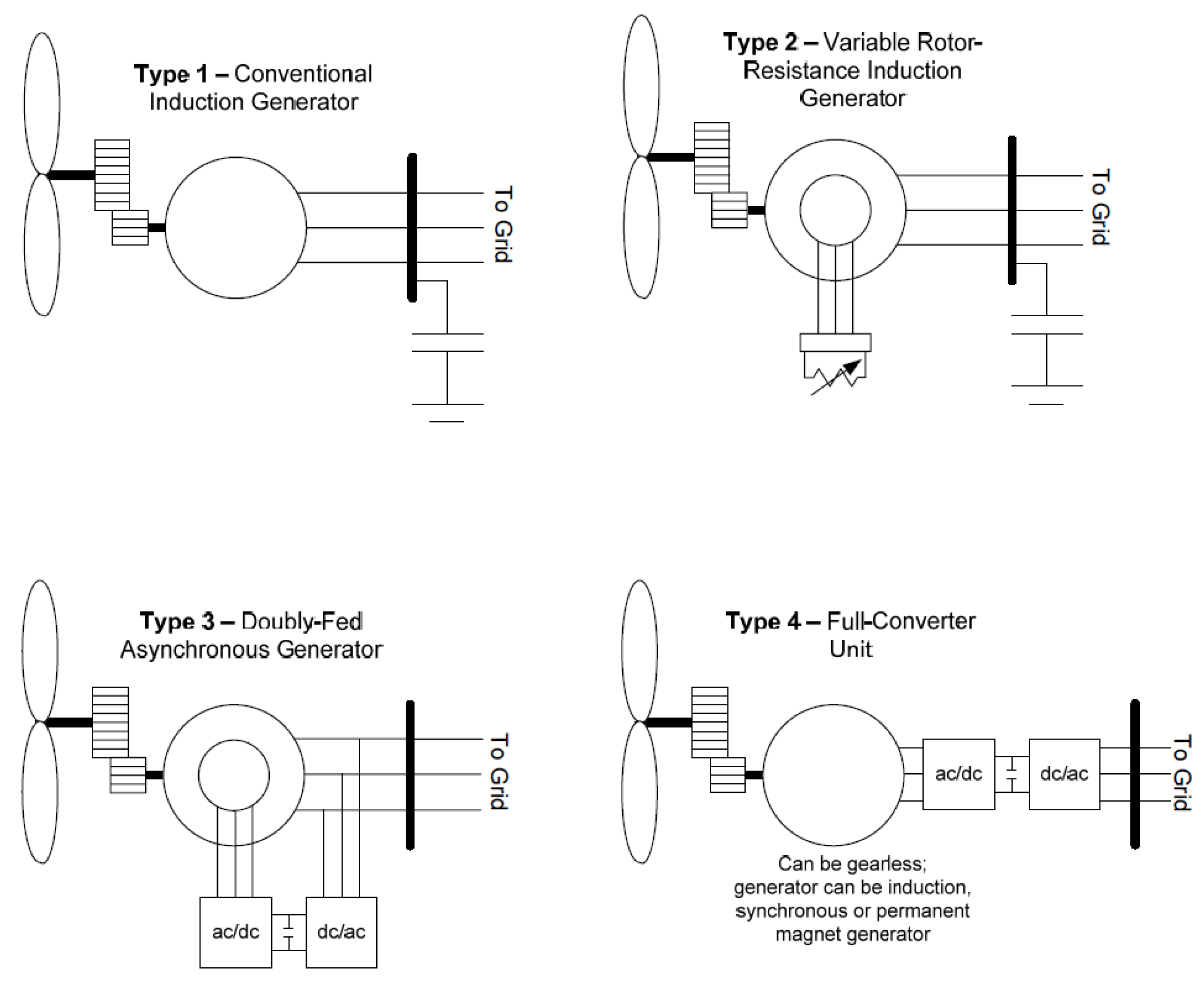
This paper focuses on Type 4 wind turbine generators (also called full converter wind turbines) due to their advantages compared to other wind turbine models.
Figure 2 shows the wind turbine generator types. As we can see from
Figure 2, the operating region of the wind turbines progressively improved between the types. In Types 1 and 2 we see the requirement of the gearbox to be effectively used depending on the wind speed as the induction generators are directly connected to the grid, resulting in lower efficiency and narrower operation region. On the other hand, in Types 3 and 4 we have converter circuits. In a Type 3 wind turbine generator, a direct connection to the grid is maintained and an additional converter path is added. Due to maintained grid connection, the control and protection of Type 3 wind turbine generators against the grid transients are complicated and require cost-intensive measures [
16]. A Type 4 wind turbine generator, however, as indicated in
Figure 2, does not need a gearbox since two-stage conversion is implemented. Therefore, the generator is connected to the grid via the converter circuit [
17]. Additionally, the control and protection mechanism can be implemented through the converter circuit which can be cost-effective compared to other types.
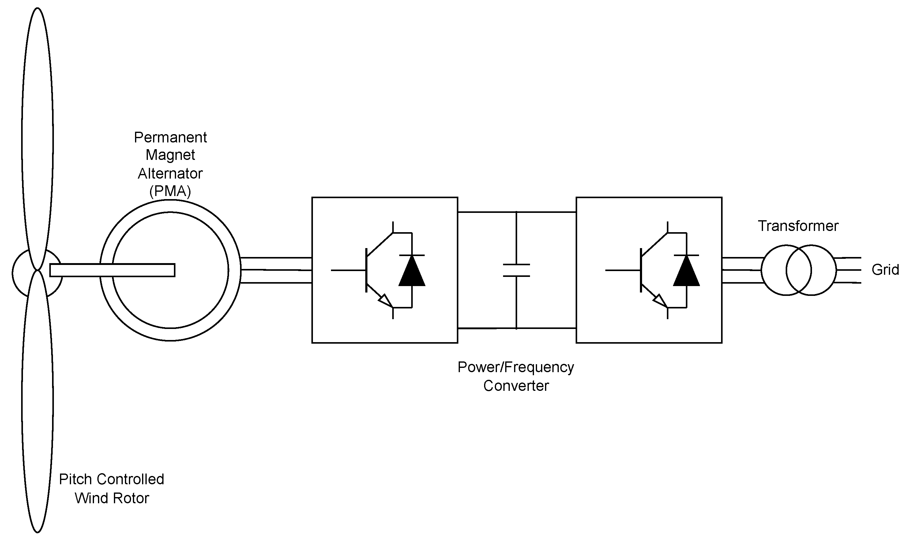
A Type 4 wind turbine generator has flexibility on the turbine and alternators since the turbine is interfaced with the grid via a power and frequency controller, as can be seen in
Figure 3. This also enables the wind turbine to operate in a wider range of wind speeds without a gearbox. Furthermore, the response of the controller to the faults is faster than other types, achieving a safer operation during transients [
18].
The behavior of synchronous machines to any disturbance is analyzed using the well-known swing equations, which use machine parameters such as inertia constant and rotor angle to determine whether or not the machine will lose synchronism with the system. In [
1,
14], synchronous machine parameters are calibrated. However, in the case of Type 4 wind turbine generators where the connection to the grid is through a fast power/frequency controller, the electrical controller, unlike in synchronous machines, reacts to the disturbance and performs an active protective measure during the fault. In this study, the Type 4 wind turbine generator is modeled using the WECC-approved REGCA1, REECA1, and WTDTA1 models [
19]. REGCA1 is the renewable generator/converter model and the WTDTA1 is the optional generic drive train model for Type 4 wind turbines. When the terminal voltage drops as a result of the fault, the electrical controller model (REECA1) detects the drop and freezes some of the simulation states. Depending on the fault type, fault duration, and the specified real and reactive current priorities, the model exhibits a different behavior which could be different than the steady-state one. After the fault is cleared, the model exhibits a recovery behavior for a specific time period, then returns back to the steady-state behavior. More detailed information about the renewable models can be found in [
17]. Since the model behavior changes during the transient event, implementing the explicit forms of the transition and observation functions
f and
h will be difficult. Therefore, rather than finding these functions explicitly, Python
TM API functions of PSS®E are utilized for simulation steps and data retrievals.
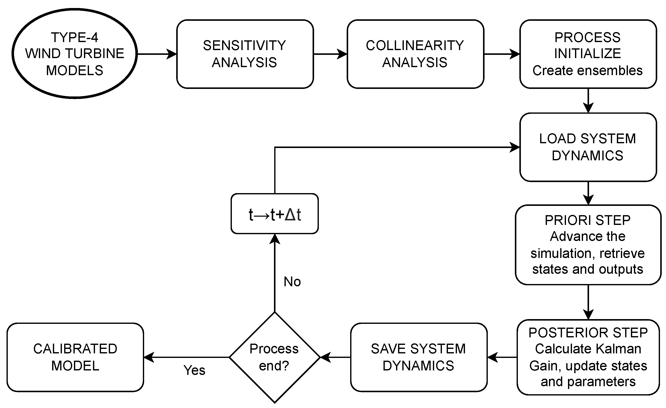
The proposed method for parameter calibration is implemented on the Type 4 wind turbine generators. The overall process can be seen in
Figure 4. Looking at the diagram, first, the working case and Type 4 wind turbine generator models are inputted into the simulation. After the sensitivity and collinearity identification, the resulting parameter set is inserted into the calibration procedure. The ensembles of the EnKF are created with Gaussian distribution. Then each ensemble’s simulation is performed for one predefined time step
in the priori step. Then in the posterior step, Kalman gain is calculated and states (and parameters) are updated. If the process does not end, it advances to the next time step.
The selected simulation tool for the calibration process is PSS®E which is a power system simulation software of SIEMENS. Using the Python
TM API of PSS®E, parallel simulation of ensembles and state and parameter updates are easily performed with well-defined function calls. As instructed in
Section 2, first a sensitivity analysis is performed for the dynamic model parameters of the Type 4 wind turbine generator. Then, unidentifiable parameters are eliminated from the subset and the collinearity analysis is performed on the remaining parameters. After removing the collinear parameters from the same subset, one can move on to the calibration process.
Since the EnKF requires N number of ensembles and their simulation to run separately, the dynamic simulation of PSS®E is paralleled for the ensembles. The method uses the event playback to decouple the power plant and increase the simulation speed. As mentioned earlier, a playback generator is placed at the POI bus, and the PMU measurements of
V and
are given as inputs to this generator via the “plbvf1” playback model. At each time step, system dynamics are loaded to the workspace via snapshot files for each ensemble. Then, the ensembles are advanced for one predefined time step. The API functions of PSS®E are used for transition function
f and the observation function
h that gives the output responses
and
. After calculating the Kalman gain and updating the states and parameters, the last versions of the ensembles are saved back to their snapshot files. Advancing the time step, the process is repeated until the end of the simulation, as shown in
Figure 4. The results of the whole process are given in the following section.
4. Results
In this section, the results of the implementation of the proposed method are given. A small-scale power system of a WSCC-9 bus network [
20] is utilized and the conventional generation power plant at bus 2 is replaced with our Type 4 wind power plant. Generic test data suggested in [
17] are used for renewable model parameters. To observe the dynamic behavior and perform the calibration, a symmetrical three-phase fault is applied at the middle of the branch between buses 4 and 6 as illustrated in
Figure 5. At the steady-state operation, the parameters of a power plant become insensitive to the output of the power plant; therefore, a transient is necessary to conduct the parameter calibration process based on the dynamic state estimation. The fault condition provides the necessary dynamic behavior, i.e., the proposed method requires measurement recordings for a fault or some other dynamics. However, the location or type of the fault is not directly related to the proposed method, such that the fault condition should only be causing the power plant to respond, and hence the output of the plant gets into a transient state. Therefore, this paper does not consider fault location or fault location observability problems.
First, the sensitivity and collinearity analyses are performed. Sensitive parameters and collinear groups among them are listed, respectively, in
Table 1 and
Table 2. Since the real-life dynamic event data for such calibration could not be found, the system shown in
Figure 5 is simulated. All the parameters of the system are assumed to be correct and active and reactive power outputs of the power plant are recorded as synthetic measurement data. Additionally, the voltage magnitude and angle at the POI where the PMU is located (also can be seen in
Figure 5) are recorded and saved to the
file for the playback generator [
19].
Calibration Results
As a next step, the parameter of interest is perturbed and then the resulting erroneous model is put into the calibration. As instructed in
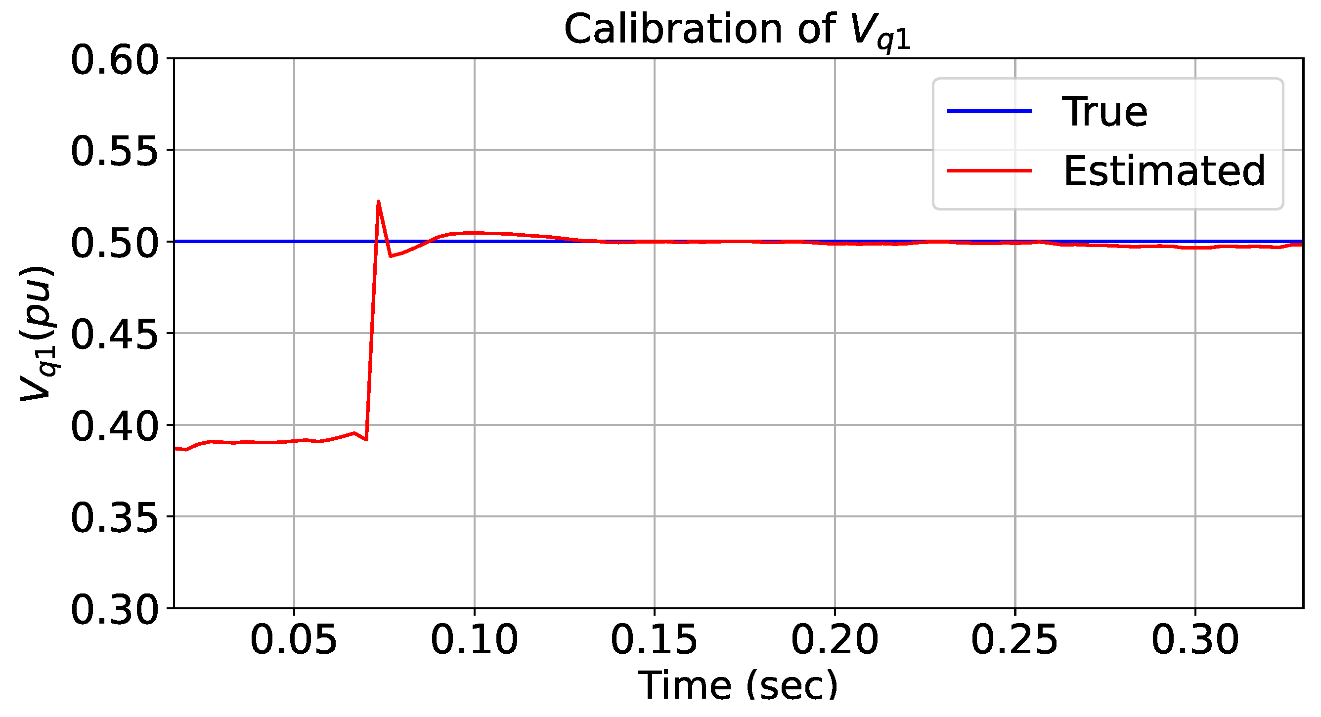
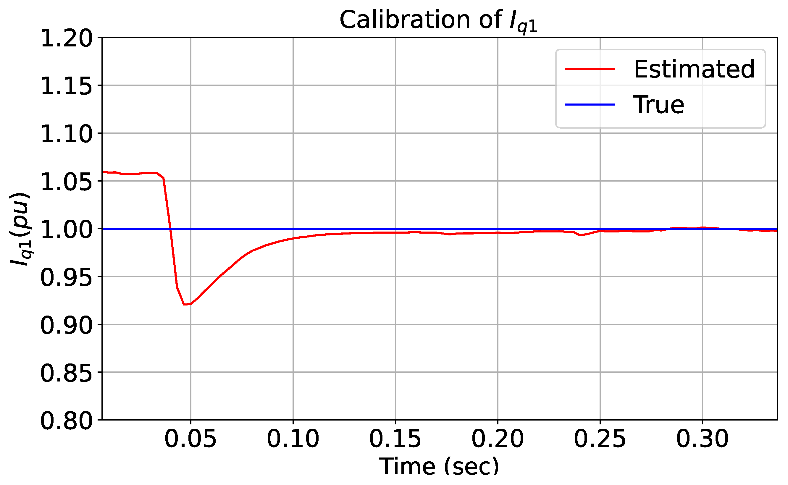
Section 3, sensitive parameters of the Type 4 wind turbine generator are calibrated separately.
Figure 6 and
Figure 7 show the transition of
and
values during the process.
, the voltage limit for high-voltage reactive current management, is one of the parameters of the REGCA1 generator model. The parameter
is one of the reactive power control parameters in the REECA1 electrical control model [
19].
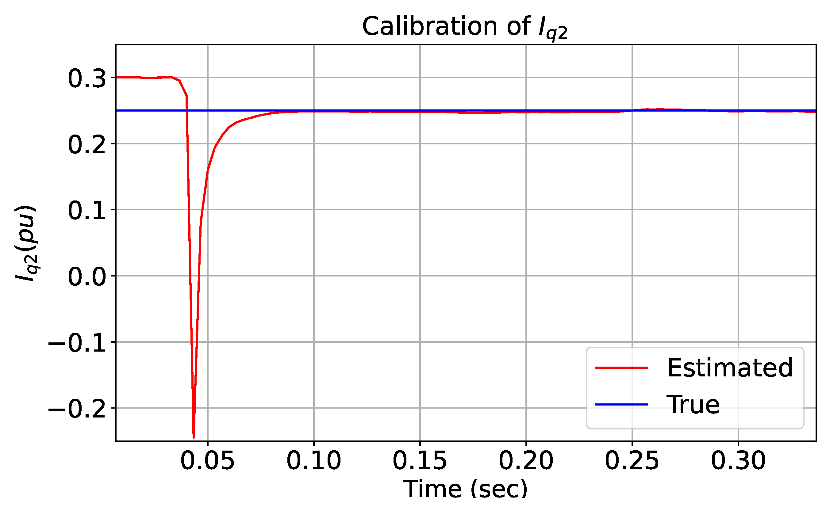
Figure 8 and
Figure 9 are the results of two other parameters of the reactive power control inside the REECA1. As can be seen in the figures, parameter calibration begins after the model starts the fault response. After the fault is cleared, even if the model and system reach the steady state (or quasi-steady state), calibration continues and the erroneous parameters are corrected.
5. Discussion
During the research on this topic, we have observed that the method works properly in the synchronous generator models studied in [
12,
14]. However, in some parameters of the Type 4 wind turbine models the method reaches the true value of the parameter, then deviations from the true value might occur as the process continues. One example of this occurrence is
, which is the converter time constant of the REGCA1 simulation model [
19]. As can be seen in
Figure 10, as the simulation continues, after the
s the parameter starts to deviate from the converged value. One of the possible reasons for this incident might be the active behavioral changes inside the model. As explained in
Section 3, the model has a discrete response to a transient event, it actively changes its behavior, freezing some of the states and activating new controls during the fault, possibly disrupting the calibration of the parameter of interest. Additionally, as can be seen in
Figure 10, the calibration occurs during the fault transient. If convergence to a value is reached during this time period, then the calibration can be terminated. Otherwise, the process will continue until the end of the simulation.
Another solution to this deviation problem might include informing the calibration tool about this mode-switching and actively interfering with the state estimation of the EnKF. However, this method would be too specific for this model and we cannot generalize this calibration method for other types of wind turbines and generators.
In this paper, calibration of the erroneous parameters of Type 4 wind turbine simulation models is performed using the Python
TM API of PSS®E. To summarize the overall process, it begins with a sensitivity and collinearity analysis of the model parameters. After the sensitive parameters are identified and collinear groups are determined, calibration is performed as the model is simulated during a transient event such as a three-phase symmetrical fault. In order to decouple the model and system dynamics and speed up the calibration process, a method called event playback is utilized and the event is replayed at the point of interconnection via a playback generator. The ensemble Kalman filter is selected for the calibration since it does not require an explicit form of the system dynamics and is easy to implement on different models for calibration. As discussed in
Section 5, in some of the parameter calibrations, the method needs a convergence criterion to finish the calibration. Further investigation and research will be carried out on this issue.


