1. Introduction
With the recent advancement in Artificial Intelligence (AI), there is a growing demand for AI-driven innovation in the healthcare domain. A key step is the design and development of data-driven models to, for instance, identify and monitor risk factors regarding chronic conditions and to support behavioural intervention for rehabilitation or prevention. The development of data-driven models requires, however, access to health data often from several sources, ranging from Electronic Medical Records (EMRs) to Personal Health Records (PHRs) from personal smartphones and smartwatches.
There are three main challenges associated with the development of AI technologies and data-driven models in the healthcare system. The first challenge concerns the data sharing of individuals (data subjects) at the personalised level as part of larger data samples, which have been highlighted in the General Data Protection Regulation (GDPR) [
1]. The data sharing at a personalised level is regulated through procedures such as ethical approvals, data protection impact assessments, and anonymisation protocols [
2]. These legislative procedures are time-consuming and subject to the complexity of the specific case study, being a potential barrier to innovation. The second challenge is connected to the availability of human subjects for prospective studies that would represent the target population. The third challenge regards the acquisition of data from these human subjects, also time-consuming and susceptible to interruptions due to unforeseen events such as pandemics, resulting in the delay or halt of the study.
The use of synthetic data mitigates the impact of these three challenges in the development of AI models [
3]. Synthetic data are an alternative way to represent the essential characteristics, such as dependencies and distributions, of real data about real human subjects. In addition, the use of synthetic data is also a privacy-preserving technique to preserve patients’ privacy and mitigate the risk of re-identification.
Previous studies addressed the design and development of synthetic data generator models for generating data under a healthcare setup (for example, electronic health records or vital signs). However, the advent of modern assistive technologies and biosensors such as smartwatches has introduced new challenges related to the specific characteristics of the signals generated by this new class of devices. Firstly, the signals obtained from wearables and biosensors are multimodal in nature. This means that variables are not sampled regularly, and their collection is strictly dependent on human activities (e.g., exercise monitored during the daytime, sleep monitored during night-time). Secondly, the acquisition of physiological biomarkers, such as the heart rate and blood pressure, is also carried out at irregular intervals. These characteristics make multimodal data a significantly hard case for existing methodologies developed for conventional time-based electronic health records sampled at regular intervals.
Addressing this specific scenario, we designed, developed, and tested two approaches for synthesising real-time multimodal physiological signals. The first is a TimeGAN-inspired [
4]
Temporally Correlated Multimodal Generative Adversarial Network (TC-MultiGAN) that generates synthetic real-time physiological signals based on physical activity, its types (such as walking or running), and the different types of physiological biomarkers at different moments of the day. This method addresses the limits of techniques derived for regularly sampled data synthesis [
4], addressing multimodal irregularities in the data collection by integrating an interpolation pre-processing step, to create time series data. The technique not only preserves the temporal correlations, but also addresses the non-uniform distribution of multimodal physiological variables throughout the day of real data. The second method presented is the
Document Sequence Generator (DSG), which synthesises physiological data by using a guided Text Generation approach. In contrast to the TC-MultiGAN, the DSG works on a chain of textual events representing the physical activity and physiological biomarkers, allowing the event occurrence at a particular time point, as well as its impact on subsequent time points. This method is agnostic to the occurrence of physiological events being timed at regular intervals. It considers the data as document sequences and applies an approach from Text Generation, by proposing an alternative mapping of the problem.
Together, these two techniques provide a viable solution to the limitations of existing solutions, when applied to heterogeneous, irregular sources of health and wellbeing data. The two solutions have a different complementary take on the problem, focusing on either (a) reconstructing the correlated phenomena represented by data reflecting their best-possible approximation through the synthetically generated data or (b) representing the data as they are preserving both the correlation and the pattern of use. These two solutions have different strengths that best fit different scenarios in a real-world setting.
Indeed, this work was developed considering multiple real case studies in the context of the H2020 flagship GATEKEEPER project on AI for digital healthcare. In line with the key issues highlighted above, the development of synthetic data generators was a contingent measure to the COVID-19 pandemic and a mitigation measure to the due diligence and lengthy negotiations required to set up a data-sharing agreement between healthcare institutions and technology providers. The presented solutions will be included within a new service for health synthetic data generation, part of the GATEKEEPER marketplace.
The rest of the paper is structured as follows.
Section 2 discusses the state-of-the-art on synthetic data generation for clinical and healthcare data. Following that,
Section 3 describes in detail our novel solutions, the TC-MultiGAN (
Section 3.2) and the DSG (
Section 3.3) and their evaluation. Then,
Section 4 discusses the issues of the comparability between the methods and the use of synthetic data for supporting innovation within our project. Finally,
Section 5 presents our final remarks.
2. Literature
The analysis of the state-of-the-art focused on five themes: (i) mathematical transformation to generate new patterns, (ii) the Synthetic Minority Oversampling TEchnique (SMOTE), a popular oversampling method to address the class imbalance problem, (iii) probabilistic models, (iv) Generative Adversarial Networks, and (v) guided Text Generation.
Random transformation methods generate new patterns through the use of specific transformation functions. A transformation function can fall into any of the time, frequency, and magnitude domains [
5]. For instance, the magnitude-domain-based data augmentation functions allow the modification of each value in a time series while keeping the time steps constant. A common example added noise to the time series signal [
6]. Other methods include, for instance, rotation [
5], scaling [
7], magnitude warping time [
8], time warping [
7], Fourier transform [
9], and spectrograms [
10]. However, these transformations do not address the time dependencies we needed to preserve in synthetic data, which can be useful for the scenario we describe. Additionally, random transformations do not preserve cross-correlations among different time-dependent and -independent variables, also a key requirement for the application of synthetic data in the development of AI-based models.
The Synthetic Minority Oversampling TEchnique (SMOTE) is an interpolation method designed to oversample the minority class within supervised learning datasets. Indeed, data imbalance is one of the most-common problems in datasets about detecting disease patterns using classification. The SMOTE has performed well in many similar time series applications such as wearable sensors [
11] and electronic health records [
12]. For time-variant datasets, the SMOTE was used in several variations, such as with deep learning [
13], the weighted extreme learning machine [
14], the furthest neighbour algorithm [
15], cost minimisation [
16], and the density-based SMOTE [
17]. However, the SMOTE was not designed to perform on unlabelled datasets such as the one used in the applicative scenarios we considered.
Probabilistic and statistical models have also been applied to synthetic data generation. In the healthcare domain, Synthea was developed under the same principle with the capability to transform data into the Hl7 Fast Healthcare Interoperability Resource (FHIR) model [
18]. Another example is the Multivariate Imputation by Chained Equations (MICE). MICE is a method based on the chained imputation of mean values regressed from existing values in the dataset. It is a cyclic method that computes until all the missing values are replaced by mean imputed regressed values [
19]. These methods are computationally fast and can scale to very large datasets, both in the number of variables and samples. Besides, they have the ability to deal with both continuous and categorical datasets by combining the use of, e.g., Softmax or Gaussian models for the conditional probabilities. However, probabilistic approaches require prior knowledge of the phenomena described by the dataset and their mutual interaction.
Generative Adversarial Network (GAN) models are an implementation of the concept of structured probabilities [
20]. GAN architectures include a Generator (G), used to compute new plausible examples based on the data distribution, and a Discriminator (D) estimating the probability of finding the generated data within the real distribution. Both the G and D are trained iteratively, until the loss function to discriminate between real and synthetic data is minimised. GAN models are among the most-common methods for generating synthetic data in the healthcare space. However, their first-generation implementations did not capture the joint correlations in the data distributions. Addressing this limitation, several GAN derivatives have been proposed. For instance, the conditional Tabular GAN (TabGAN) uses convolutional neural networks and prediction loss to improve the correlation among the variables [
21]. The TabGAN works with mode-specific data normalisation for non-Gaussian data distributions while training the Generator to deal with imbalanced discrete columns [
22]. This model was further improved in the TGAN, preserving mutual information among health record columns [
23]. Most of these GAN models use Long Short-Term Memory (LSTM) in order to develop the Generator, which is able to capture the record pattern based on the temporal context.
The ability to capture the local pattern and the temporal context is the key feature required to generate the short-term synthetic data of wearables for physical and physiological monitoring. Convolutional Neural Networks (CNNs) with LSTM have been used to capture local patterns based on the temporal context. This type of architecture is also used by DeepFake to generate simulated ECGs [
24]. A comprehensive model combining ECG with cardiovascular diseases, the SLC-GAN [
25], was developed using this type of architecture. However, these architectures do not capture the temporal correlation among multiple variables. The existing GAN approaches for temporal data, the TimeGAN [
4], adapt the GAN architecture to the generation of regular time series.
To sum up, most of the existing GAN models require either tabular formats or signals sampled uniformly as the input. This requirement conflicts with how wearables and biosensors operate and the real-life data acquisition patterns, e.g., several times a day and bundled in different formats based on the different scenarios of use. Real-life data are susceptible to (a) usage patterns and (b) human routine reflected in the irregular data sampling of the physical and health status. The large number of missing covariates at specific time points of real data limits the applicability of existing methodologies. Differently, the two techniques we propose were designed from the ground up on real-life data.
The rest of the paper discusses the two approaches we developed to address this gap in existing methods for multimodal health data, specifically learning from an irregular sampling of different variables and generating synthetic data comparable in terms of temporal correlations between variables and irregular sampling.
3. Techniques for Real-Time Multimodal Physiological Signal Synthesis
This section describes two complementary approaches addressing the above-mentioned issues of existing methods.
The Multimodal Generative Adversarial Network (TC-MultiGAN) adopts the TimeGAN architecture capable of learning and preserving the temporal correlation from the irregular sampling of different variables while generating regular synthetic data that can support the development of AI models for health. To this end, the TC-MultiGAN has two main steps: (1) encoding the categorical data from physical activity types at different hours of the day and (2) estimating the absence of independent variables (e.g., physical activity variables such as sleep and exercise) as zero and interpolating dependent physiological status (e.g., heart rate).
The Document Sequence Generator (DSG) synthesises data based on text sequencing (such as FHIR health documents) and uses text embeddings to support flexible synthetic data generation, preserving both the variable correlations and the irregularity of the seed to support the development and testing of AI infrastructures. The DSG encodes sequences of variables at different time points as
characters and
text. Approaches based on text sequencing include automated summarisation of individual patient records [
26], question and answer, and clinical entity recognition [
27].
Both methods can be used with health native document formats such as JSON FHIR, instead of tabular formats, which can provide a great convenience in supporting fast innovation in the space of AI for health.
The evaluation of these techniques used the Bilingual Evaluation Understudy (BLEU) score [
28]. BLEU score compares the machine-generated text to a set of reference translations or texts and calculates the n-gram overlap between the two. The resulting score is between 0 (worst) and 100 (perfect). A comparable study on clinical entity recognition reported a BLEU-4 score of 32.29 for charRNN and 77.28 for GPT-2 [
27]. Other methods involve guided Text Generation, which refers to the process of generating text with the help of additional input or guidance. This has been in several forms, including:
Conditional Text Generation [
29]: This involves providing a model with some context or information, such as a prompt or a topic, and asking it to generate text based on that context.
Text completion [
30]: This is similar to conditional Text Generation, but instead of a prompt, the model is provided with partially completed text and is asked to complete the text.
As EHRs are patient-centric, we propose to combine Conditional Text Generation and text completion in a Gated-Recurrent-Unit (GRU)-based [
31] character Recurrent Network (charRNN) framework.
3.1. Datasets
The seed dataset combines smartphones’, self-assessments’, and wearables’ data collected in the scope of the GATEKEEPER project’s large-scale pilot. The dataset included smartwatch-generated physiological signals such as heart rate, calories burned and exercise activity, sleep activity (duration and type), and classic electronic medical records such as diagnostics, collected from patient questionnaires. The dataset was provided as bundles of JSON documents in Fast Healthcare Interoperability Resources (FHIR) [
32] format. The FHIR bundles included metadata about the type and time of observations using the LOINC standard.
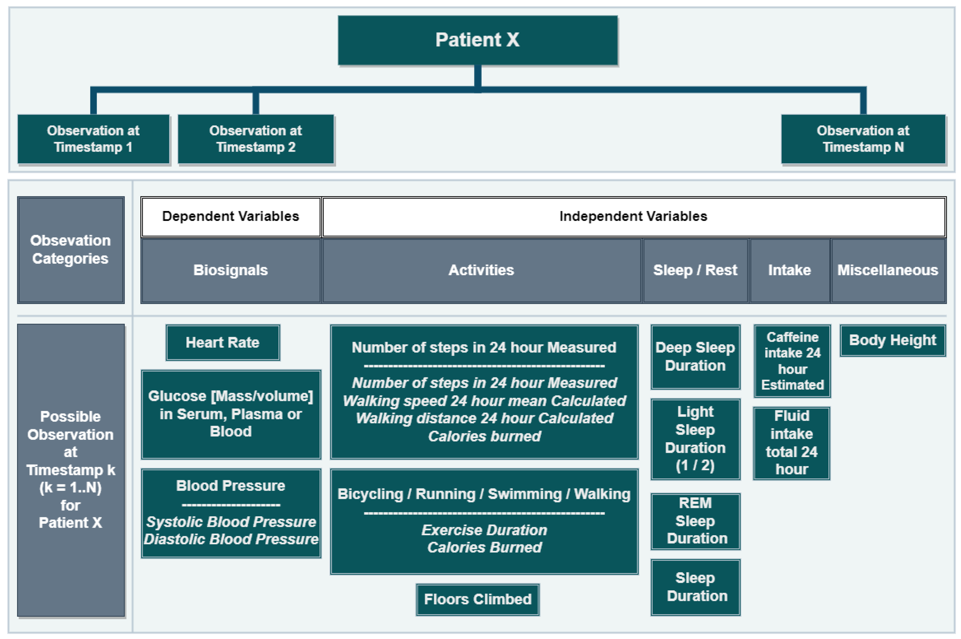
FHIR observations can be as simple as a single record or compound, combining several observations. For example, heart rate measures are simple observations, while walking activities are compound, including the walking duration and calories burned. Observations in the dataset concerned biosignals (25%), activities (9%), sleep/rest (65%), and food/liquid intake (1%). The dataset included both independent and co-dependent variables as simple or compound observations, collected at different times of the day for a variable period of time; see
Figure 1.
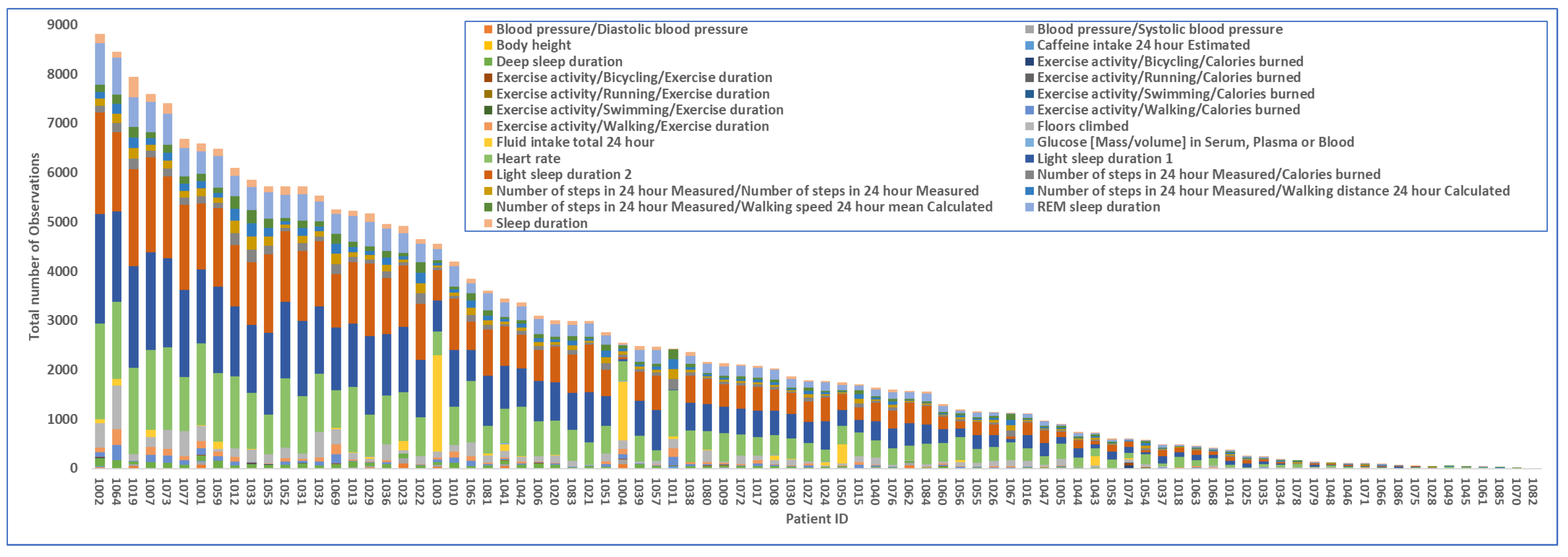
The dataset represented 86 unique patients and a variety of observations collected in periods that ranged from a few days to six months. As anticipated in
Section 3, the dataset did not present the regularity required for applying the existing approaches to synthetic data generation. Indeed, each patient’s data collection followed a unique pattern in terms of type, frequency, and gaps in the data points. For instance, the patient data collection in
Figure 2 showcases the high variability in the data collection of real patients. Specifically, the patient in
Figure 2 alternated periods of high- and low-volume recording and periods of regular use with gaps of days.
To sum up, the analysis of the dataset highlighted four types of irregularities in relation to (1) the number of observations per patient and their type, (2) the duration of the data collection per patient, (3) the period of continuous recording and gaps, and (4) the number of observations per day. For instance, the number of produced observations per patient varied greatly with 18 of 85 (21.18%) scoring above the median of 4k total observations; see
Figure 3.
In line with the EU and U.K. GDPR, the dataset has not been released as the explicit consent of the data subjects was not collected.
3.2. TC-MultiGAN
We developed the Temporally Correlated Multimodal GAN (TC-MultiGAN), derived from the TimeGAN [
4] architecture, to synthesise irregularly sampled physical and electronic health records based on encoded hours and activity types while training temporal probabilities of individual variables and conditional probabilities among dependent and independent variables (
Figure 4). The TC-MultiGAN objective formulation for data synthesis was designed for variable intensities and a joint temporal distribution at irregular intervals. Firstly, we defined the dependent (biosignals) and independent (sleep/rest, activity type, and intake) variables’ spaces acquired from the seed. Secondly, we performed categorical encoding of the time based on different times of the day and week as the activity types would be different at different times of the day. Thirdly, we performed interpolation on dependent biosignals to derive the optimisation functions in correlation with irregularly sampled activity types. Fourthly, we derived the embedding function to represent the temporal dynamics to a lower feature space followed by reconstruction and generator functions to convert random noise to synthetic data based on the formulated objective. The generated data would be compared with the seed via a discriminative function. This was an iterative procedure, which continued till the values from the loss functions reached below the threshold level. The details are illustrated in
Figure 4.
3.2.1. Data Pre-Processing
Let Y be the seed for training the probabilistic distribution and dependencies. Each variable v present in and has the distinguished sampling rate s.
Considering that biosignals are dependent on the activity types, intake, and sleep/rest (see
Figure 1), we assigned symbol
to the independent variables (activity types, intake, sleep/rest, and encoded time) and
to the dependent biosignals (vital signs, heart rate, blood pressure, etc.). Both
and
have variable time stamps
with sampling rate
s for each variable
v. Furthermore, we performed categorical encoding of the time so as to represent different times of the day, as well as to include in
. The temporal probabilistic distributions of both
and
from the real data seed were trained along with their temporal dependencies for the generation of synthetic data closer to the real seed distribution (see
Figure 4). The data from the wearables were converted into the FHIR format, with each value of the variable having a separate timestamp in a JSON structure. The JSON was converted into a tabular format required to train the GAN, which included numerous
null values. To address the excess of
null values, we performed linear interpolation on the heart rate values due to their continuous nature, whereas we assigned 0 to null values in
and calories burned due to their fixed intervals.
3.2.2. TC-MultiGAN Objective Formulation
Let be the random noise vector, which can be instantiated with specific values. We considered tuples of the form , where m is the total number of variables, s is the sample number of variable v in the and categories, and n is the time of the sample taken. There were two objectives to generate the synthetic data:
Matching the joint distribution of random data with the seed at the global level: This can be achieved by learning the density
that can best approximate
from the real data. This can be prevented by minimising the distance
D among two probabilities as follows:
Note that
and
are two temporal variables whose conditional probability needs to be compared.
Matching the joint distribution at the local temporal level: This can be achieved by minimising the distance between two conditional probabilities for any time
t. This can be represented as follows:
3.2.3. TC-MultiGAN’s Networks
For the TC-MultiGAN, we derived four networks to transform the random noise into synthetic data. This is an iterative procedure that requires four networks:
- i
The Embedding Network allows irregular temporal mappings from the seed feature space to the latent space.
- ii
The Generator Network converts random values with the total dimensions of and in the seed feature space to the embedding space.
- iii
The Discriminator Network receives the output from the embedding space and performs differentiation between the reconstructed data and the seed.
- iv
The Reconstruction Network transforms the latent space back to the feature space to provide the final synthesised output.
The workflow involving the four networks is represented in
Figure 4. Firstly, we define the
Embedding Network, where
and
denote the latent space corresponding to
and
. The Embedding Network
takes temporal features from both
and
and converts them into their embeddings. Considering the conditional dependencies of
over
at irregular time intervals, we used time encoding and interpolation to parameterise the latent space of
(biosignals) according to the latent space of
(activity type and time encoding). We implemented the embeddings using a 3-layer forward directional Long Short-Term Memory (LSTM) with the total number of hidden neurons defined as equal to the total number of samples in the temporal sequence (
N). LSTM can be described as
For the
Generator Network, we define random sequences via a Gaussian distribution as
and
for both variable types, respectively. We implemented the Generator Network
with
dependent on
. The embedding space of random sequences can be represented as follows:
The
Discriminator Network receives the output from the embedding network and returns the classification among individual variables
v, in both
and
as
. They are represented by the following equations:
Note that
and
denotes the sequences of hidden states in both the forward and backward directions;
are LSTM functions;
,
are output classification functions. Finally, the
Reconstruction Network was implemented as
.
3.2.4. Optimisation Functions
While performing sequence embedding and generating synthetic data, we developed loss functions that jointly iterate along embedding, reconstruction and generation functions to update random sequences with respect to the real seed probabilistic distribution. Firstly, the reconstruction loss function
minimises the probabilistic distance between the real seed and the synthetic data generated, described as follows:
The second loss function minimises the loss for the likelihood of the classification of the synthetic data’s individual variable distribution in both
and
in order to generate the synthetic variable in the future space. This can be represented as follows:
The purpose of having the loss function
is to minimise the conditional probabilities between the real seed and the synthetic data generated at the temporal level, described as
3.2.5. Experimental Results
Evaluation Metrics We assessed the performance of the TC-MultiGAN using the following evaluation measures:
The
Wasserstein distance [
33] is the distance function defined between probability distributions on a given metric space M. This can be represented as
where
and
are Cumulative Distribution Functions of
U of size
m and
V of size
n.
The
Kolmogorov–Smirnov (KS) Test [
34] defines a 2-sample nonparametric test of the equality of probability distributions. It can be represented as
The
Jensen–Shannon distance [
35] computes the distance between two probability arrays. This can be defined as
where
D is the Kullback–Leibler divergence and
m is the pointwise mean of
and
.
The
Distance Pairwise Correlation [
36], in contrast to the previous metrics, measures differences in pairwise correlations among variables. This can be stated as
where
n represents the number of variables.
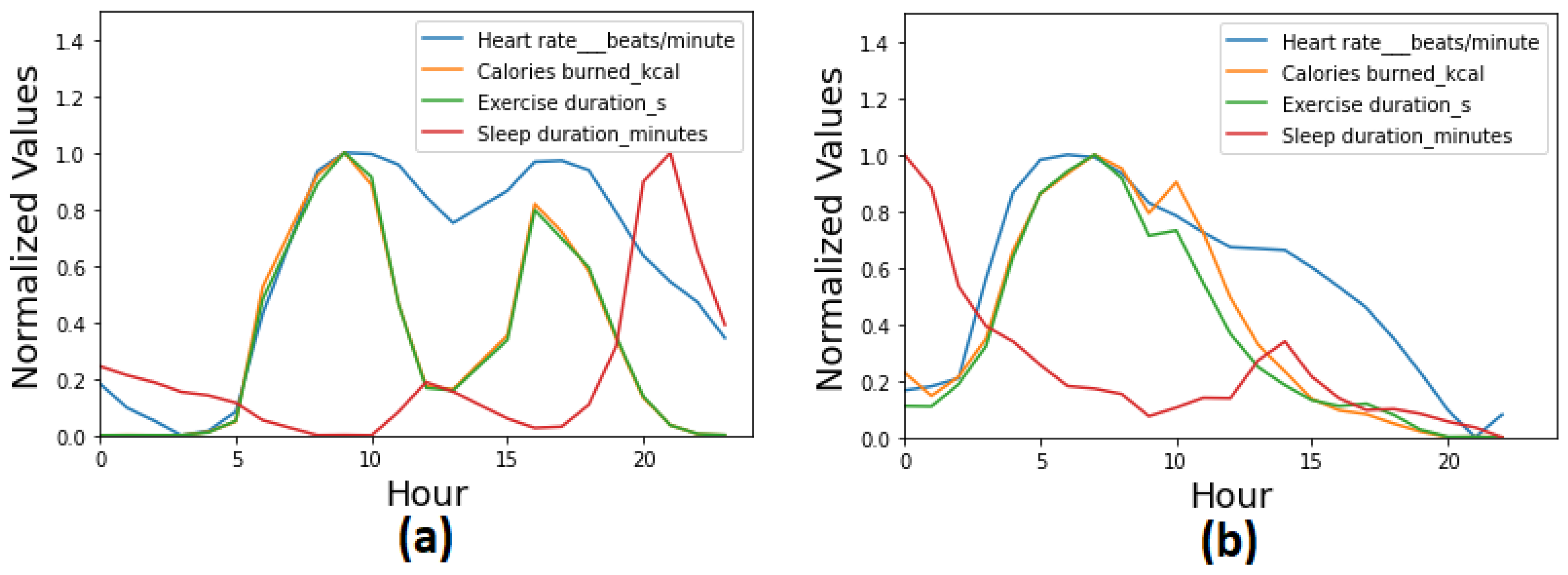
Statistical Evaluation We performed a statistical evaluation of the TC-MultiGAN in three steps. Firstly, we performed a descriptive analysis and a comparison between the real and synthetic datasets. The comparison was performed across different physiological variables (e.g., heart rate, sleep activity, physical activity, etc.) across 24 h. The results are presented in
Table 1 and
Figure 5. The table and the figure show a significant similarity between the real data and the synthetic data generated while preserving the temporal correlation across different times and spaces. Both the figure and the table show a higher heartbeat during daytime and high physical activity, whereas a lower heartbeat during sleep activity and the night-time.
In the second step, we performed a statistical comparison based on the evaluation metrics described in
Section 3.2.5 while synthesising a different number of users via the TC-MultiGAN. The results are presented in
Table 2, which shows consistency in the differences between the real and synthetic data while generating a different number of users ranging from 10 to 200.
In the third and last step, we performed a state-of-the-art comparison of the TC-MultiGAN with existing approaches (
Table 3). The results showed that the TC-MultiGAN outperformed all the existing approaches that are based on the probabilistic distribution of the individual variables only. This showed that encoding and training the temporal correlation was the key to synthesising real-time physiological signals close to the real dataset.
3.3. Document Sequence Generator
The DSG considers the training data as sequences of characters and documents, rather than time series, for instance an observation about a heart condition followed by observations about physical activities such as step counts. As such, the developed solution uses Recurrent Neural Networks, as described in the rest of this section.
3.3.1. RNNs
Recurrent Neural Networks (RNNs) [
40] allow training of any sequential data patterns, ranging from temporal data to text (sequences of characters). The TC-MultiGAN model just presented requires the interpolation of missing values in a tabular format: an assumption about what is not described by the seed. Differently, the DSG makes no assumptions about the gaps in the data collection and could best fit the application scenarios whether the phenomena at hand cannot be reasonably interpolated, such as social activities and events that would suddenly emerge (no-trend-based). As such, the DSG treats the seed data sequences as
textual sequences.
3.3.2. Approach and Rationale
The problem was approached using the SEQ2SEQ technique [
41] to train the observations using a character-level approach. Each observation in the seed was split into a number of characters, representing the input sequences. The corresponding targets contained the same number of characters, but shifted one character to the right. The targets represent the output sequence. The model architecture was initialised with random data. We trained our model such that we could learn the relationship between the input and output sequences.
The model needs to address two questions concerning time and activities:
Given a timestamp and observation activity, what is the next timestamp and activity?
Given a timestamp and observation activity, what is the value associated with that activity?
The developed solution focuses on the latter as preliminary experiments failed to identify a model for the first question. However, we found a workaround by adapting a guided Text Generation approach. We trained the model using irregular time intervals and observation codes as contextual information. This solution considered the observations of each patient as a whole document. It reframed the goal of a single model as the ability to create either part of or a whole full document, with a similar probability distribution as the seed. The input for each observation was part of the synthetic patient data that the model was attempting to generate.
The process in
Figure 6 is iterative and articulated into (1) pre-processing, (2) model training, (3) Text Generation, and (4) evaluation, as described in the following sections. The results were evaluated at the end of each cycle; the model hyper-parameters were updated, and the model was retrained until evaluation reached a target BLEU score [
42] and an overall acceptable 2-sample Kolmogorov–Smirnov test (KS test) [
34] result.
3.3.3. Pre-Processing
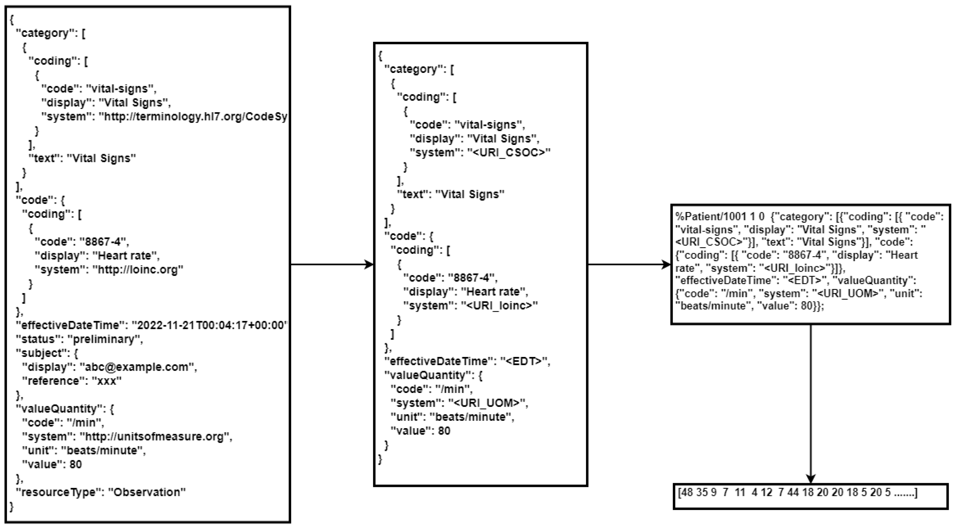
The pre-processing step converts the text into a numerical representation (
Figure 7). However, to give the model the best chance of learning the signals, the pre-processing performed the compression of the notation of the FHIR format. Indeed, the FHIR observation included metadata fields that were not significant for the purpose of synthetic data generation, which would negatively impact the computational resources required and the size of the model. The compression shortened verbose identifiers (see
Table 4) and removed all repeated and redundant references, for example:
"resourceType": "observation";
"status": "preliminary"
The values of effectiveDateTime, effectiveTiming, and valuePeriod encode the time of the observation. Before the optimisation steps described above, these values were stored in a time index recording the patient’s unique identifier ID, the observation number N, and the elapsed time in seconds t. ID N was then attached at the head of the stringified JSON representation.
Finally, the JSON strings were tokenised, breaking the text into individual characters. For example, the word “{"code: ” would be tokenised into the following characters:
“{”, “c”, “o”, “d”, “e’, “ ”. The characters were then converted into a numerical vector used as the input for training the model. An example of the pre-processing is shown below (
Figure 7).
The final pre-processing step (tokenisation) used the
TextVectorization layer in Tensorflow Keras (Tensorflow library
https://www.tensorflow.org/, accessed on 1 December 2022) on a cloud infrastructure. As such, the data ingested in this last step should be carefully considered as the meta-data of the vectorised data become part of the model pipeline.
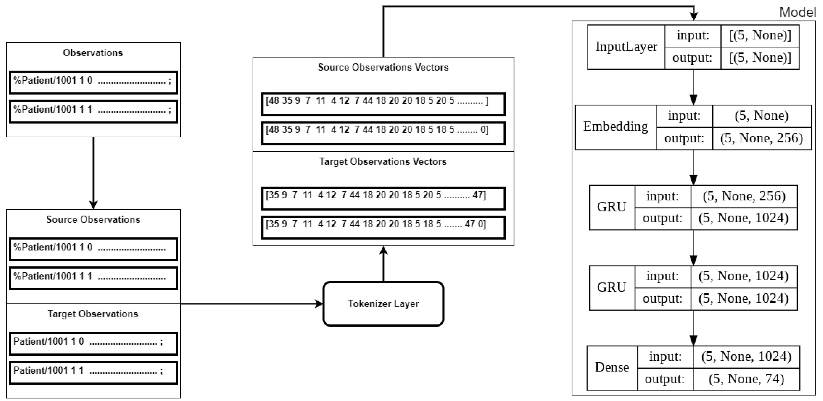
3.3.4. Model Training
Similarly, the execution of the model training was implemented in Python using the Tensorflow Keras library. The model architecture consisted of three hidden layers: an Embedding Layer and two GRU layers (see
Figure 8). The
sparse categorical loss function was used to minimise the loss. The output from the training of the model was the Tensorflow
logits [], which were used to generate the predictions. The model was designed to retain up to 187 characters at each step. If the observations were less than 187 characters, the sequence was padded with zeros in the tokenisation step.
In our experiments, the final sparse categorical loss recorded was 0.096 after 50 epochs of training. The model with the final weights and the Tokeniser Layer were saved to be deployed as a module of the synthetic data generation infrastructure.
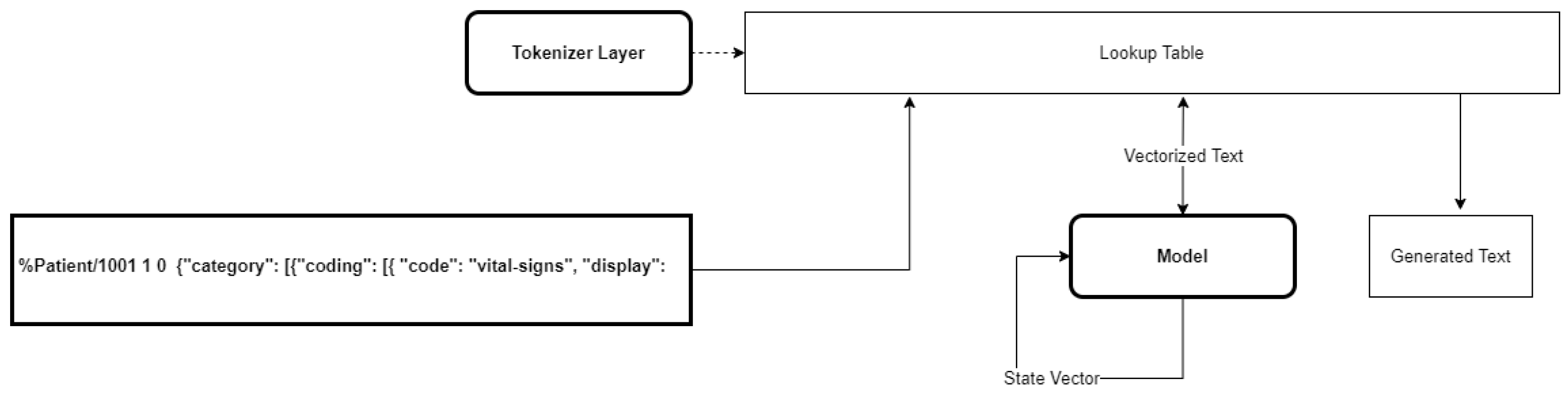
3.3.5. Text Generation
Text was generated using the prediction method of the model, as shown in
Figure 9. Text Generation is also an iterative process: each round trip produces an array of Tensorflow
logits corresponding to a character in our vocabulary. The randomness of the predictions was controlled by scaling the
temperature of the logits before applying a softmax function, following the technique used in Natural Language Generation to improve the model diversity [
43].
3.3.6. Evaluation
The evaluation was carried out using
sacreBLEU [
42], a BLEU-score Python package, mapping the pre-processed raw data as the reference text and the generated text as the hypothesis. The sacreBLEU package implements a BLEU score on
4-grams. The final BLEU scores were evaluated at the model temperatures of
0.9 and
1.0, with the results reported in
Table 5.
The BLEU scores were acceptable, ranging from an average of 57 to 98 on a 0–100 scale. This was a better performance than the scores of 32.29 for the charRNN and 77.28 for GPT-2 reported in [
27]. However, the BLEU score is a parameterised metric, depending heavily on the seed text and how the seed text is pre-processed [
42]. Next, we wished to confirm that the probability distribution of the values in the generated data was sound with the seed.
As per the previous solution, we used the 2-sample Kolmogorov–Smirnov test (KS test) [
34] for a sample of patients. For a particular observation category or sub-category, we tested the null hypothesis that the seed and the synthetic data were generated from the same probability distribution. We determined the critical KS value using a significance level of 0.05 for each instance, and we did not reject the null hypothesis if the calculated KS value was less than the critical KS value. The results reported in
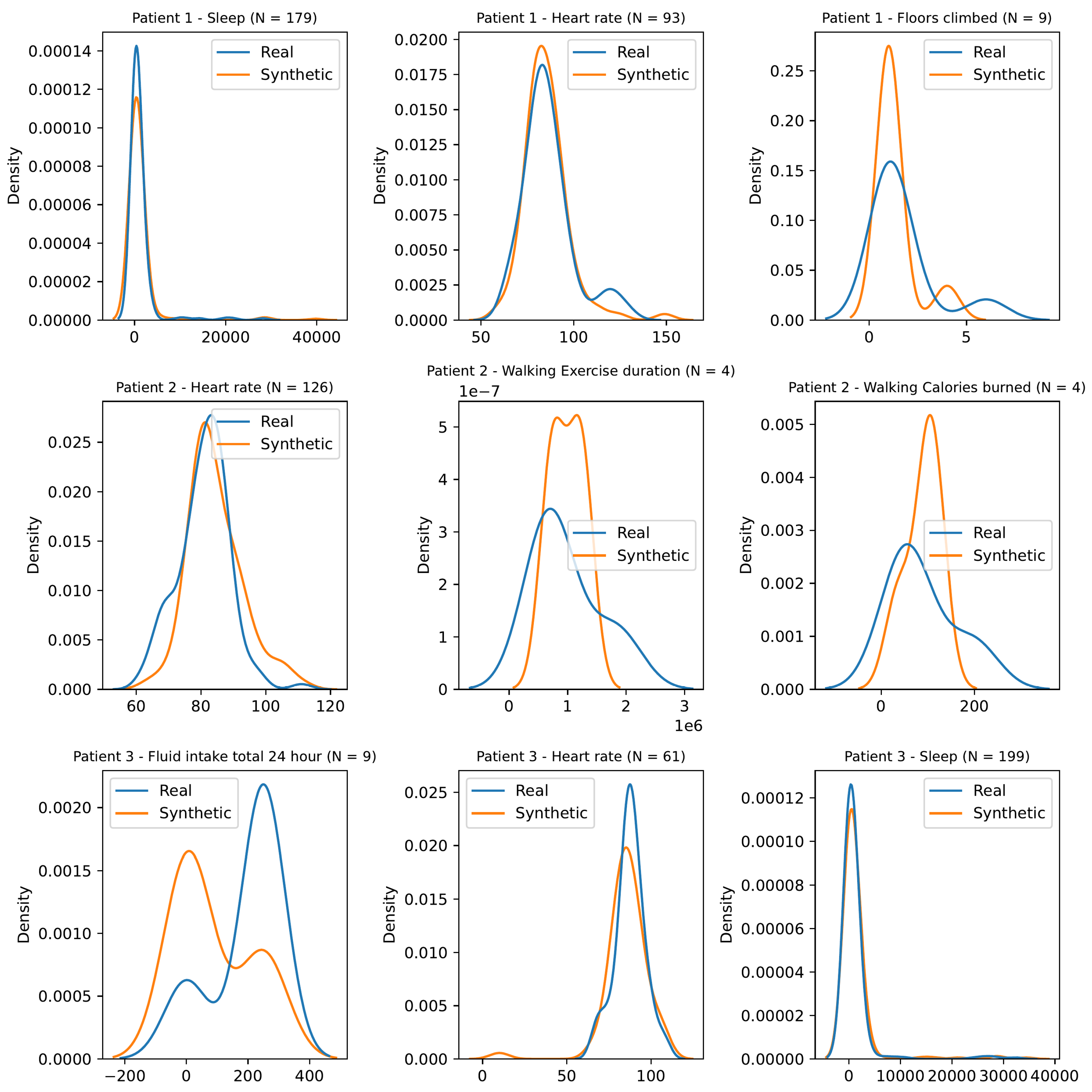
Table 6 and the distributions shown in
Figure 10 indicated that the model can be used to generate synthetic data with a similar probability distribution as the seed.
4. Discussion
The presented solutions addressed the gaps in the currently available techniques for synthetic data generation for healthcare, specifically targeting a real-life setting involving personal devices. The two techniques approach the problem differently. The first solution addresses a well-known limitation of existing GAN-based architectures on the properties of input data, i.e., tabular data with regular timestamps. It introduces an interpolation and time encoding step to address the data synthesis with multimodal irregular timestamps. The second solution introduces a novel use of RNNs in a new domain, through a new mapping of the problem as character prediction and text sequencing, which contrast with existing approaches focusing on tabular synthesis. Furthermore, the solution introduces a workaround to limit the prediction of the time of the next activities, by the self-feeding of synthetic patients data as context prompts.
4.1. Evaluation and Comparability
Both solutions were tested using a range of evaluation metrics in line with the state-of-the-art and demonstrated the ability to retain the correlation between the multimodal multi-feature irregular real data used as the seed. The evaluation was embedded within the training cycle of the models and/or their use. In the first case, the TC-MultiGAN uses a discriminator to identify and discard low-quality data and an information loss function to inform the advancement in the model training. The time encoding step allowed preserving the temporal correlation at different times of the day. As a result, TC-MultiGAN outperformed the existing state-of-the-art approaches such as the CGAN [
23], Gaussian interpolation [
37], Dragan GAN [
38], or Cramer GAN [
39]. Although the Cramer GAN had the lowest distance pairwise correlation, it did not manage to have a probability distribution comparable to the data seed. Our TC-MultiGAN had both a pairwise correlation, as well as a probabilistic distribution compared to the data seed.
The second model evaluates the model by comparing the generated data with the training set, using the same BLEU score metrics during both the training and use phases. The first key difference between the two approaches to evaluation is the presence of the discriminator in the first solution. The discriminator discards “bad” records while attempting to mimic the real data, while the second model leaves the choice to the data user. This difference is the result of how the GAN architecture works: the synthetic “good” data are often included in the training set to follow the training cycles, and as such, it is necessary to keep the generated data sound with the original training set.
A second difference between the two approaches is in the quality of the input data. In the first case, the input is a time series, where significant estimations are made to transform irregular sequences into regular temporal signals, while the second case models a mixed bag of irregular heterogeneous observations. It is important to highlight the direct connection between the approach to the evaluation and the characteristics of the training data. As such, the comparability of the results from models using different datasets is still an open issue.
The case of the two presented models extended this difference to how these datasets are used and for what purpose. Intuitively, the two models consider edge cases differently, or in other words, the sparse data are differently reflected in the trained model. On the one hand, the focus of the first model is the physiological phenomenon that the model should learn from the data, identifying what can best mimic the real data. On the other hand, the focus of the second model expands to the human factor behind the data, reflecting the imperfect dynamics of how real data are generated.
As such, the comparability of the two solutions should be framed as a matter of quality, factoring the purpose of the model and the use of the synthetic data. Intuitively, this issue directly relates to documenting the synthetic data generation services in light of how different actors would use the synthetic data, supporting the evaluation of end-users.
From a general perspective, generated data that are too close to the original training set could pose a risk of involuntary disclosure of personal data or even the re-identification of data subjects. As such, the evaluation strategy must take into account these two competing needs: avoiding involuntary disclosure while representing the health and wellbeing phenomena as close as possible to what is represented by the real data.
4.2. Application in GATEKEEPER and Beyond
In the scope of the GATEKEEPER project, the presented models have been implemented to generate the datasets for AI model design and development based on physical activity adherence to the WHO rules. Yet, they can be used to synthesise the data based on the target population for specific reference use cases such as the Type 2 diabetes risk engine, understanding the impact of physical activity on cancer survival subjects, physical activity recommender systems, etc. Specifically, the TC-MultiGAN can be used to generate vital signs (e.g., ECGs) in correlation with blood glucose measurements for non-invasive glycaemic event detection modelling. In contrast, the Document Sequence Generator can be used to augment irregular temporal patterns such as health questionnaires, which can often have missing values due to the lack of user input.
These two solutions are currently being integrated within a new GATEKEEPER service for synthetic data generation. This service will also include the CoolSim (CoolSim software
https://github.com/GATEKEEPER-OU/coolsim, accessed on 1 December 2022), a multi-agent simulator combining a fully customisable probabilistic model and models developed using Synthea (Synthea software
https://synthetichealth.github.io/synthea/, accessed on 1 December 2022), an off-the-shelf data generation library for generating single-dimension synthetic data. This new service should become available from the GATEKEEPER marketplace by the end of 2023.
5. Conclusions
We identified issues emerging from the analysis of real-life datasets and gaps in existing synthetic data generation approaches. Our applications for SDG require generating data to train AI models for healthcare and supporting the development of AI infrastructures. On the one hand, synthetic data should preserve the temporal correlation between several variables learned from multimodal irregular data well enough for an AI medical device. On the other hand, synthetic data must preserve other characteristics of real-life data concerning the correlation between the observations and activities of daily living that can stress and validate infrastructures for real-world deployment.
These two requirements are hard to achieve through one solution. As such, we developed two complementary approaches that best address different needs at different stages of developing AI services for healthcare.
The two models were both tested with results that were comparable to the state-of-the-art. Furthermore, the flagship H2020 GATEKEEPER project and its large-scale pilot provided the opportunity to validate both approaches in the real-life software development of a wide range of AI services. The source code of the two solutions is publicly available for reuse (
https://github.com/GATEKEEPER-OU/synthetic-data, accessed on 1 December 2022 and
https://github.com/ABSPIE-UOW/GATEKEEPER/synthetic-data, accessed on 1 December 2022).
This contribution highlights the need to surpass an evaluation of methods only on benchmarks and performances. Indeed, the two proposed solutions both present strong points and limitations. However, while considered within a development life-cycle, both have a role at different stages of development and for different tasks. An open issue concerns how to document the “quality” of these models in light of specific tasks rather than agnostic evaluations based on the comparisons between the synthetic and training sets.
The GATEKEEPER experience highlighted that synthetic data generation has a crucial role in enabling and accelerating the development of breakthroughs. Indeed, synthetic data find use in a wide variety of activities, from the design of new models to their testing. Furthermore, synthetic data have a privacy-preserving application, creating a shield between data subjects and data consumers. This characteristic can open up the healthcare data space to new actors mitigating the risks and costs related to the bottleneck of data-sharing agreements.
However, synthetic datasets and models do not cancel the risks of re-identification. As far as we know, this risk is less prominent than the potential benefit of using synthetic data generators as a privacy-preserving layer for AI and data-driven applications. However, future work should focus on including privacy by design techniques and checks within the architecture of synthetic data approaches.

 ,
, 


