Self-Supervised Learning for Online Anomaly Detection in High-Dimensional Data Streams

Abstract

In this paper, we address the problem of detecting and learning anomalies in high-dimensional data-streams in real-time. Following a data-driven approach, we propose an online and multivariate anomaly detection method that is suitable for the timely and accurate detection of anomalies. We propose our method for both semi-supervised and supervised settings. By combining the semi-supervised and supervised algorithms, we present a self-supervised online learning algorithm in which the semi-supervised algorithm trains the supervised algorithm to improve its detection performance over time. The methods are comprehensively analyzed in terms of computational complexity, asymptotic optimality, and false alarm rate. The performances of the proposed algorithms are also evaluated using real-world cybersecurity datasets, that show a significant improvement over the state-of-the-art results.

1. Introduction

Anomaly detection, that can be summarized as detecting unexpected data patterns [1], has many real-world applications, such as cybersecurity [2,3,4], hardware security [5], medical health care [6], surveillance videos [7], aviation [8], transportation [9], power systems [10], and time series problems [11]. A detected anomaly may be a sign of an unwanted and often actionable event, such as a cyber-attack, suspicious human behavior, system failure, etc. In many applications, the timely and accurate detection of abnormal data patterns is crucial as it allows for proper countermeasures to be taken in a timely manner to counteract any possible harm. For example, the quick detection of an abnormal behavior observed in the telemetry observations of a spacecraft could prevent a catastrophic loss [12].

The online learning of anomalies in a self-supervised fashion, as they are detected, can facilitate the fast and accurate detection of the same anomaly type when it happens again. Such self-supervised training without requiring human-labeled instances can greatly improve the detection performance over time. While deep neural network-based methods have been quite popular in many machine learning tasks, including anomaly detection [13,14,15], they are not amenable for continually learning new anomaly types in an online fashion due to catastrophic forgetting [16]. As they try to learn new patterns in an incremental fashion, they tend to forget the previously learned patterns. However, statistical methods that require lightweight training, such as neighbor-based methods, can continually learn new patterns in an online fashion [17].

In this work, we consider the timely detection and learning of anomalies in high-dimensional data-streams. Multivariate anomaly detection techniques can detect anomalies that are manifested in the interactions between several data-streams that cannot be detected by the univariate detection methods [18]. For instance, detecting and mitigating a stealthy distributed denial-of-service (DDoS) attack requires the joint monitoring of multiple data-streams [4,19]. This in turn, leads to the high-dimensionality challenge, i.e., an effective anomaly detection technique that needs to be scalable for high-dimensional data in real time.

Motivated by the aforementioned reasons, we propose a neighbor-based, online, multivariate anomaly detection (NOMAD) technique that can handle high-dimensional and heterogeneous data in real-time, and that lends itself to a performance analysis.

Contributions: Our contributions in this paper can be summarized as follows:

• Two variations of a data-driven, neighbor-based, and sequential anomaly detection method called NOMAD are proposed for both semi-supervised and supervised settings depending on the availability of the data;
• The computational complexity and asymptotic false alarm rate of NOMAD are analyzed, and a procedure for selecting a proper decision threshold to satisfy a desired false alarm rate is provided;
• A self-supervised online learning scheme that can effectively detect both known and unknown anomaly types by incorporating the newly detected anomalies into the training set is introduced;
• Finally, the performance of the proposed methods are evaluated in two real-world cybersecurity datasets.

The rest of the paper is organized as follows. Related works are discussed in Section 2. In Section 3, the mathematical formulation of the considered anomaly detection problem and the relevant background information are provided. We present the proposed anomaly detection and learning methods, along with the theoretical analysis of the performance and the computational complexities in Section 4. The experiments are presented in Section 5. Finally, we conclude the paper in Section 6.

2. Related Work

Anomaly detection has been extensively studied in various domains. For instance, an SVM-based approach for anomaly detection was proposed in [20]; several theoretical information measures were proposed in [21] for the intrusion detection problem; and two new information metrics for DDoS attack detection were introduced in [3]. With the new challenges, such as high-dimensionality, heterogeneity, and real-time detection posed by emerging applications (e.g., internet of things, smart city, intelligent transportation systems, etc.), there is still a significant need for studying the new challenging aspects of the anomaly detection problem.

Real-time detection can be better addressed by sequential anomaly detection techniques compared to the outlier detection techniques [1]. As opposed to considering each instance independently, sequential methods also take the history of observations into account. The cumulative sum (CUSUM) detector [22] is a well-known sequential change detection technique that assumes probabilistic models for nominal and anomalous data points, and computes the cumulative log-likelihood-ratio (LLR) over time, declaring an anomaly if the statistic exceeds a predefined threshold. The accuracy of assumed models, as well as the estimated parameters, are the key factors in the performance of CUSUM and more general parametric methods. CUSUM is the minimax optimum under the condition that the probability distributions before and after the change are completely known [23]. However, this is not possible in many real-world applications with a priori knowledge of the underlying distributions. Estimating the probability distributions quickly becomes intractable for high-dimensional data that includes many unknowns, such as the anomaly onset time, the subset of anomalous dimensions, etc., in addition to the parameters of the nominal and anomalous models. To tackle this complexity, ref. [24] proposed a relaxed version of CUSUM, in which each data-stream is assumed to be independent of others. However, this univariate method is not suitable for detecting changes in the correlation between data-streams. A sequential test for detecting changes in the correlation between variables, as well as localizing the highly correlated variables in high-dimensional data-streams was proposed in [25]. This is a parametric method based on the assumption that the observed vectors are multivariate Gaussian distributed. It is proposed solely for the detection of correlation changes between data-streams and does not generalize for other changes in the distribution. In this paper, we are interested in detecting general changes in unknown distributions, including the changes in the correlation structure.

Neighbor distance-based methods are geometric methods that are based on the assumption that anomalous data instances occur far from the nominal instances. For instance, refs. [26,27] have proposed non-parametric outlier detection techniques based on the minimum volume set (MVS) of the nominal data. MVS corresponds to the region of greatest probability density with minimum data volume, and is known to be useful for anomaly detection [28] based on the assumption that anomalies occur in the less concentrated regions of the nominal dataset. These non-parametric outlier detection methods estimate the MVS of nominal training samples using neighbor graphs, and declare a data point as anomalous if it lies outside the MVS. Despite being scalable to high-dimensional and heterogeneous data, they do not consider the temporal anomaly information, and thus are prone to higher false alarm rates compared to sequential anomaly detection methods. Similarly, ref. [29] proposed a neighbor graph-based method that computes an anomaly score for each observation and declares an anomaly by thresholding the score value. In this paper, as opposed to the outlier detection methods that treat a single outlier as an anomaly, we consider an anomaly to consist of persistent outliers and investigate the sequential and non-parametric detection of such anomalies using the temporal information in data-streams. Recently, ref. [30] proposed a non-parametric neighbor-based sequential anomaly detection method for multivariate observations. This method computes the test statistic based on the number of neighbor edges at different splitting points within a window and stops the test whenever the test statistics exceed a threshold. Due to its window-based nature, this method has inherent limitations in achieving small detection delays. It also recomputes the neighbor graphs at every time instance and for every splitting point; therefore, its computational complexity is not suitable for real-time applications. In another recent work, ref. [31] proposed a distance-based and CUSUM-like change detection method for attributed graphs. Attributed graphs are first mapped into numeric vectors, and then the distance between the mean response of an observation window and the mean response of the training data are computed via a CUSUM-like sequential algorithm. In addition to the limitations arising from the window-based nature of the method, the local relations between samples are disregarded due to considering only the mean response of the training set. As a result, in the cases where training data have a multimodal distribution, this method will not be effective. As compared to [31], we take into account the local relations between the data instances.

In addition to classical machine learning techniques, such as the PCA-based [32], KNN-based [30,33], exponential weighted moving average [34], and feature bagging networks [35], deep neural networks have recently become popular in anomaly detection, as in other machine learning fields. For instance, a deep auto encoder-based detection method was proposed in [36]. The deep auto encoder, that first encodes the inputs to a compressed representation, and then decodes the original inputs from the representations, is trained on nominal data and is expected to have small reconstruction errors when faced with nominal data during testing. Interestingly, for anomalous data, it is expected to produce statistically larger errors. It raises alarm if the majority of the instances within a window have reconstruction errors larger than a threshold and are marked as anomalous. Another auto encoder-based anomaly detection method was proposed in [37]. A generative adversarial network (GAN) is an effective deep neural network architecture for learning to generate samples from a complex probability distribution. In [38], the authors used a convex combination of reconstruction error and discriminator error of the GAN to compute an anomaly score for each instance. Similarly, the MAD-GAN algorithm proposed in [39] uses a combination of reconstruction and discriminator errors of the LSTM-based GAN.

3. Problem Formulation

Suppose that a system is observed through d-dimensional observations ${\mathcal{X}}_t=\{x_1,x_2,\dots ,x_t\}$ in time. The objective is to detect an anomaly occurring at an unknown time $\tau$ as soon as possible while satisfying a false alarm constraint. This problem can be formulated as a change detection problem as follows:

$$\begin{array}{cc}\hfill & f=f_0,t<\tau ,f=f_1(\ne f_0),t\ge \tau ,\hfill \end{array}$$

(1)

where f is the true probability distribution of observations and $f_0$ and $f_1$ are the nominal and anomaly probability distributions, respectively. The objective of the problem is to find the anomaly time T that minimizes the average detection delay while satisfying a false alarm constraint, i.e.,

$$\underset{T}{inf}{\mathsf{E}}_{\tau }\left[{(T-\tau )}^{+}\right]\mathrm{subject}\mathrm{to}{\mathsf{E}}_{\infty }\left[T\right]\ge \beta ,$$

(2)

where ${\mathsf{E}}_{\tau }$ represents the expectation given that change occurs at $\tau$, ${(.)}^{+}=max(.,0)$, and ${\mathsf{E}}_{\infty }$ denotes the expectation given that no change occurs, i.e., ${\mathsf{E}}_{\infty }\left[T\right]$ denotes the expectation of the false alarm period.

Lorden’s minimax problem is a commonly used version of the above problem [40], in which the goal is to minimize the worst-case average detection delay subject to a false alarm constraint:

$$\underset{T}{inf}\underset{\tau }{sup}\mathrm{ess}\underset{{\mathcal{X}}_{\tau }}{sup}{\mathsf{E}}_{\tau }\left[{(T-\tau )}^{+}\right|{\mathcal{X}}_{\tau }]\mathrm{s}.\mathrm{t}.{\mathsf{E}}_{\infty }\left[T\right]\ge \beta ,$$

(3)

where “ess sup” denotes the essential supremum. In simple words, the minimax criterion minimizes the average detection delay for the least favorable change-point and the least favorable history of measurements up to the change-point while the average false alarm period is lower-bounded by $\beta$.

4. Proposed Methods

Neighbor-based methods maintain their popularity due to their competitive performance, computational efficiency, analyzability, and interpretability [41,42]. In this section, we present our k-nearest-neighbor (kNN) based NOMAD algorithm, extensively analyze its computational complexity, and provide an asymptotic upper bound on its false alarm rate. Then, we also propose a supervised extension for NOMAD for the cases where training data are available for some anomaly settings. Finally, we introduce a unified framework for the two NOMAD detectors.

The intuition behind using kNN distance for anomaly detection is the similarity between the inverse kNN distance and likelihood. Specifically, for $f\left(x_i\right)\ge f\left(x_j\right),x_i,x_j\in \mathcal{X}$, it is expected that the distance $g_k\left(x_i\right)$ of $x_i$ to its kth nearest neighbor in $\mathcal{X}$ is smaller than that of $x_j$. This probability increases with the size of $\mathcal{X}$, i.e., ${lim}_{\left|\mathcal{X}\right|\to \infty }P(g_k\left(x_i\right)\le g_k\left(x_j\right))=1$. This, in turn provides grounds for using the difference of kNN distances in NOMAD to approximate the log-likelihood ratio.

4.1. NOMAD Algorithm

In the training phase, assuming a training set ${\mathcal{X}}_N$ consists of N nominal data instances using the kNN distances $\left\{g_k\left(x_m\right)\right\}$ between each node $x_m\in {\mathcal{X}}_N$ and its k nearest neighbors, NOMAD finds a baseline statistic that represents a boundary between the observations under nominal operations and the tail events under nominal operations at significance level $\alpha$. Then, in the test phase, it compares the kNN distances $g_k\left(x\right)$ between test data instance $x$ and its k nearest neighbors in ${\mathcal{X}}_N$ with the boundary statistic to compute negative/positive anomaly evidence for observation $x$, and accumulates it over time for reliable detection. Roughly, the greater $g_k\left(x\right)$ is, the less likely $x$ comes from the same distribution $f_0$ as the nominal points.

Specifically, in the training phase, NOMAD ranks the points in ${\mathcal{X}}_N$ in ascending order $\{x_{\left(1\right)},\dots ,x_{\left(N\right)}\}$ in terms of the total distance:

$$L_m=\sum _{n=1}^k{g}_n{\left(x_m\right)}^{\gamma },$$

(4)

where $g_n\left(x_m\right)$ is the distance between point $x_m\in {\mathcal{X}}_N$ and its nth nearest neighbor in ${\mathcal{X}}_N$, k controls the nearest neighbors in the calculation of the total distance, and $\gamma >0$ is the weight. The first K points with the smallest total distances $\{L_{\left(1\right)},\dots ,L_{\left(K\right)}\}$ represents the denser parts of the data distribution, and the $L_{\left(K\right)}$ is selected as the borderline total distance, separating the dense area from the tail evenly. K is chosen as $K=\lfloor N(1-\alpha )\rfloor$, where $\lfloor ·\rfloor$ is the floor operator.

In the test phase, for each data instance $x_t$, NOMAD firstly computes the total distance $L_t$ with respect to the training set ${\mathcal{X}}_N$, as in Equation (4). Then, it computes the anomaly evidence that could be either positive or negative by comparing $L_t$ with the borderline total distance $L_{\left(K\right)}$

$$D_t=log{L}_t^d-log{L}_{\left(K\right)}^d,$$

(5)

where d is the number of data dimensions. $D_t$ is a measure of how well the observation fits the nominal distribution. Finally, it updates a detection statistic ${\mathrm{\Delta }}_t$ that accumulates the anomaly evidence $D_t$ over time, and raises an anomaly alarm the first time ${\mathrm{\Delta }}_t$ crosses a predefined threshold,

$$\begin{array}{c}\hfill \begin{array}{cc}\hfill {\mathrm{\Delta }}_t& =max\{{\mathrm{\Delta }}_{t-1}+D_t,0\},{\mathrm{\Delta }}_0=0,\hfill \\ \hfill T& =min\{t:{\mathrm{\Delta }}_t\ge h\}.\hfill \end{array}\end{array}$$

(6)

The NOMAD procedure is summarized in Algorithm 1.

Algorithm 1 The proposed NOMAD procedure

1: Input:${\mathcal{X}}_N,k,\alpha ,h$ 2: Initialize:$\mathrm{\Delta }\leftarrow 0,\mathrm{t}\leftarrow 1$ 3: Training phase: 4: For each $x_m\in {\mathcal{X}}_N$ compute $L_m$ as in Equation (4) 5: Find $L_{\left(K\right)}$ by selecting the Kth smallest $L_m$ 6: Test phase: 7: while$\mathrm{\Delta }<\mathit{h}$do 8:        Get new data $x_t$ and compute $D_t$ as in Equation (5) 9:        $\mathrm{\Delta }=max\{\mathrm{\Delta }+D_t,0\}$ 10:        $t\leftarrow t+1$ 11: $\mathrm{Declare}\mathrm{Anomaly}$

4.2. Analysis of NOMAD

Theorem 1.

As $N\to \infty$, for a given threshold h, the false alarm period of NOMAD is asymptotically lower-bounded by

$$\begin{array}{cc}\hfill {\mathsf{E}}_{\infty }\left[T\right]& \ge e^{{\omega }_{0}h},\hfill \\ \hfill {\omega }_0& =v_d-\theta -\frac{1}{B}\mathcal{W}\left(-B\theta e^{-B\theta }\right),\hfill \\ \hfill \theta & =\frac{v_d}{e^{v_d{L}_{\left(K\right)}^d}},\hfill \end{array}$$

(7)

where ${\omega }_0>0$, $\mathcal{W}(·)$ is the Lambert–W function, $v_d=\frac{{\pi }^{d/2}}{\mathrm{\Gamma }(d/2+1)}$ is the constant for the d-dimensional Lebesgue measure (i.e., $v_d{L}_{\left(K\right)}^d$ is the d-dimensional volume of the hypersphere with radius $L_{\left(K\right)}$), and B is the upper bound for $D_t$.

Proof. 

See Appendix A. □

The bound B for $D_t$ is obtained from the training data. The Lambert–W function is easily computed with built-in functions in popular programming languages, such as Python and MATLAB. Note that Equation (7) gives an upper bound on the false alarm rate (FAR) since

$$\mathrm{FAR}={\mathsf{E}}_{\infty }{\left[T\right]}^{-1}\ge e^{-{\omega }_{0}h},$$

which can be used to select a threshold value h to satisfy a false alarm constraint $\beta$:

$$h=-log\beta /{\omega }_0.$$

(8)

Due to its sequential nature, the parameters of NOMAD control the fundamental trade-off between minimizing the average detection delay and false alarm rate. Parameter k determines how many nearest neighbors to take into account when computing the total distance $L_m$, given by Equation (4). A smaller k would result in it being more sensitive to the anomaly, hence it supports the earlier detection, but at the same time it causes it to be more prone to the false alarms due to nominal outliers. A larger k would result in the opposite. $0<\gamma <d$ is the weight that determines the emphasis on the difference between the distances.

The alarm threshold h in Equation (6) directly controls the trade-off between minimizing the detection delay and false alarm rate. Decreasing h will yield smaller detection delays, i.e., earlier detection, but also more frequent false alarms. It is typically selected to satisfy a false alarm constraint, as shown in Equation (8). The significance level $\alpha$ is at a secondary role supporting h. For a fixed h, a larger $\alpha$ would result in smaller detection delays, but also more frequent false alarm, since more nominal data points will lie outside the selected dense area.

Complexity: Next, we analyze the computational complexity of our proposed method. The training phase of NOMAD requires the kNN distances between each pair of the data points in the training data to be computed. Therefore, the time complexity of the training phase is $O\left(N^{2}d\right)$, where d and N are the dimensionality and size of the training data, respectively. The space complexity of the training is $O\left(dN\right)$, since N points are stored for testing. Note that training is performed once offline, thus, the time complexity of online testing is usually critical for scalability. In the test phase, computing the kNN distance of a test point to all points in the training data takes $O\left(dN\right)$ computations. Since the test statistic is updated recursively, the space complexity of testing is not significant. Consequently, the proposed NOMAD algorithms linearly scale with the number of data dimensions d in both training and testing. It also linearly scales in the online testing with the number of training points.

Computing the nearest neighbors of a query point is the most computationally expensive part of the algorithm, as the distance to every other point in the train data needs to be computed before the k smallest of them is selected as the k nearest neighbor. As the dimensionality increases and the training size grows, the algorithm becomes less efficient in terms of the running time. The computational complexity of the algorithm can be reduced by approximating the kNN distance rather than computing the exact value. Due to the inaccuracy introduced at the approximated kNN distances, NOMAD’s performance will drop compared to that of when using the exact kNN distances. However, depending on the system requirements, e.g., the sampling rate and importance of timely detection, and the gain from the improvement in running time by employing kNN approximation can compensate for the exact distances. To evaluate the performance of the method, in approximate and exact kNN scenarios, we adopted a kNN approximation algorithm [43] that is scalable for high dimensional data.

In a simulated experiment, we evaluate the performance and computation time of our algorithm in both scenarios. The experiments are carried out in MATLAB on an Intel 3.60 GHz processor with 16 GB RAM. In simulations, the data dimensionality is 50, and the training size is 500,000. The anomaly is manifested by a shift in the mean of the observations by three standard deviations in $10\%$ of the dimensions. The performance of the original and efficient NOMADs are shown in Figure 1. The average computation time (computation of Equations (5) and (6) per observation) for both is also summarized in the

Table 1. Average computation overhead of the original and efficient NOMAD per sample.

Average Execution Time (s)
ExactkNN	FastkNN
0.075	0.0054

. As shown by results, approximating the kNN distance decreases the computational overhead; however, at the cost of a small loss in the performance. In the experiment, the average running time per observation using the approximation method dropped by a factor of 14. The versions with exact and fast kNN computations can run in real-time at a speed of 13 samples per second and 185 samples per second, respectively.

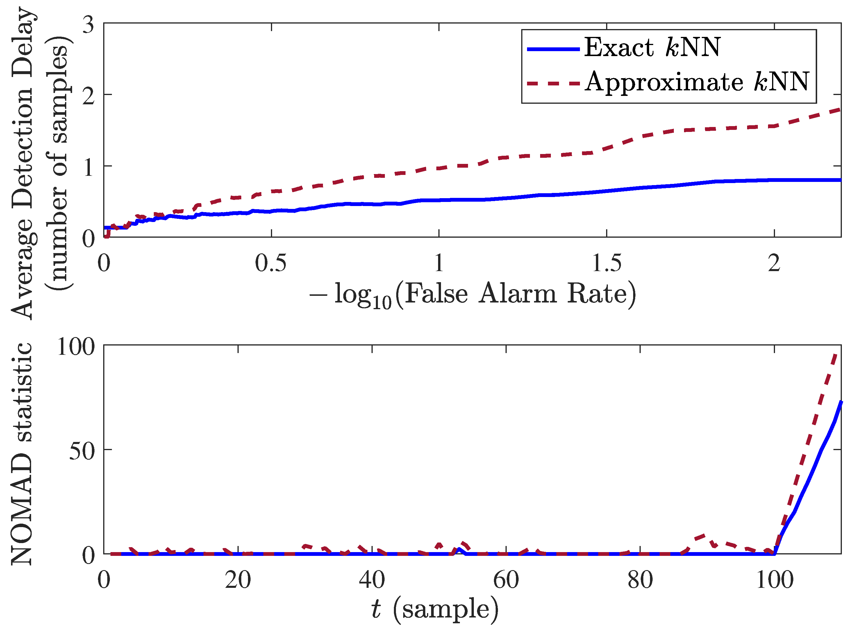
4.3. An Extension: NOMADs

In this section, we consider the case of having an additional anomaly training dataset along with the previously discussed nominal dataset. Next, we extend the NOMAD method to take advantage of the anomaly dataset in order to improve its performance. Consider an anomaly training set ${\mathcal{X}}_{M^{\prime }}^{\prime }=\{x_1^{\prime },x_2^{\prime },\dots ,x_{M^{\prime }}^{\prime }\}$ in addition to the nominal set ${\mathcal{X}}_N=\{x_1,x_2,\dots ,x_N\}$. In this case, the anomaly evidence for each instance can be computed by comparing the total distance $L_t$ with respect to the nominal dataset with the total distance $L_t^{\prime }$ with respect to the anomalous dataset. Thus, there is no need to learn the borderline total distance $L_{\left(K\right)}$ in training to be used as a baseline for $L_t$ in testing (cf. Equation (5)). That is, no training is needed for NOMADs. However, before testing, a pre-processing might be required to remove the data points that are similar to the nominal training set. The reason for cleaning the anomaly dataset rather than the nominal dataset is that usually, the anomaly dataset is obtained by collecting observations from a known anomalous event that may typically include nominal observations too. For instance, in a network intrusion detection system (IDS), after the occurrence of an attack, several observations could still be of nominal nature. The cleaning step is carried out by finding and removing the data points of the anomaly training set that lie in the dense area of the nominal training set,

$${\mathcal{X}}_M^{\mathrm{clean}}={\mathcal{X}}_{M^{\prime }}^{\prime }\backslash \{x_m^{\prime }\in {\mathcal{X}}_{M^{\prime }}^{\prime }:L_{x_m^{\prime }}\le L_{\left(K\right)}\},$$

(9)

where $L_{x_m^{\prime }}$ is the total distance of $x_m^{\prime }$ with respect to the nominal points in ${\mathcal{X}}_N$. Hence, the training procedure of NOMAD that finds $L_{\left(K\right)}$, can be used for preprocessing the anomalous training data.

While testing for each testing data instance $x_t$, the anomaly evidence is calculated by

$$D_t=d(log{L}_t-log{L}_t^{\prime })+log(N/M),$$

(10)

where $L_t$ and $L_t^{\prime }$ are the total distances of $x_t$ computed using Equation (4) with respect to the points in ${\mathcal{X}}_N$ and ${\mathcal{X}}_M^{\mathrm{clean}}$, respectively; and N and M are the number of points in the nominal and (cleaned) anomalous training sets. The statistic update and decision rule of NOMADs are the same as in NOMAD, given by Equation (6). In the NOMADs procedure, and different from Algorithm 1, Equation (10) is used in line 9 to compute the anomaly evidence $D_t$.

In practice, there is a typical imbalance between the sizes of the nominal and anomaly training sets due to the inherent difficulty of obtaining anomaly samples. Since the total kNN distances in a dense nominal set ${\mathcal{X}}_N$ are expected to be smaller than those in a sparse anomaly dataset, for an anomalous data point, $L_t$ can be smaller than $L_t^{\prime }$, resulting in negative anomaly evidence, that can lead to poor detection. In order to deal with the imbalance of datasets, the term $log(N/M)$ in Equation (10) acts as a correction factor. Specifically, for $N>M$, $log(N/M)>0$ compensates for $L_t$ being unfairly small compared to $L_t^{\prime }$. This correction factor naturally appears in the asymptotic optimality proof, as shown next.

Theorem 2.

When the nominal distribution $f_0\left(x_t\right)$ and anomalous distribution $f_1\left(x_t\right)$ are finite and continuous, as the training sets grow, the NOMADs statistic $D_t$, given by Equation (10), converges in probability to the log-likelihood ratio,

$$D_t\stackrel{p}{\to }log\frac{f_1\left(x_t\right)}{f_0\left(x_t\right)}\mathrm{as}M,N\to \infty ,$$

(11)

i.e., NOMADs converges to CUSUM, which is the minimax optimum in minimizing the expected detection delay while satisfying a false alarm constraint.

Proof. 

See Appendix B. □

4.4. Unified Framework for Online Learning

The availability of the labeled training data is a major limiting factor for improving the performance of anomaly detection techniques. In several applications, obtaining a comprehensive and accurate labeled training dataset for the anomaly class is very difficult [1]. In contrast, in most applications, a typically sufficient amount of comprehensive nominal training data is available. Semi-supervised techniques, including NOMAD, constitute a popular class of anomaly detection methods that require labeled training data only for the nominal class. These techniques try to build a model of nominal operation/behavior. Hence, anomaly detection is performed by detecting data that significantly deviate from the constructed nominal model. Supervised techniques, moreover, assume availability of both nominal and anomalous datasets, and build models for classifying unseen data into nominal vs. anomaly classes. NOMAD, as a supervised technique, outperforms the semi-supervised NOMAD technique for the known anomaly types, as shown in Section 5. However, NOMADs, and in general supervised anomaly detectors, may fall short of detecting unknown anomaly types while NOMAD, and in general semi-supervised anomaly detectors, can easily handle new anomaly patterns as they do not depend on assumptions about the anomalies.

Combining the strengths of NOMAD and NOMADs, we propose a self-supervised online learning scheme called NOMADo, that is capable of detecting new anomaly types and at the same time is capable of improving its performance for detecting the previously seen anomaly types. Particularly, in the unified NOMAD method, both NOMAD and NOMADs run in parallel to detect anomalies, and the anomalous data instances first detected by NOMAD are included in the anomalous training set of NOMADs in order to empower the detection of similar anomaly types. Since the NOMADs procedure involves all of the necessary elements for NOMAD, there is no further computation overhead induced by the unified approach. Keeping track of the cumulative decision statistics of NOMAD and NOMADs, the unified NOMAD scheme, NOMADo, stops the first time either NOMAD or NOMADs stops:

$$\begin{array}{cc}\hfill {\mathrm{\Delta }}_t^{\left(1\right)}& =max\{{\mathrm{\Delta }}_t^{\left(1\right)}+D_t^{\left(1\right)},0\},\hfill \\ \hfill {\mathrm{\Delta }}_t^{\left(2\right)}& =max\{{\mathrm{\Delta }}_t^{\left(2\right)}+D_t^{\left(2\right)},0\}\hfill \end{array}$$

(12)

$$\begin{array}{cc}\hfill T& =min\{t:{\mathrm{\Delta }}_t^{\left(1\right)}\ge h_1\mathrm{or}{\mathrm{\Delta }}_t^{\left(2\right)}\ge h_2\},\hfill \end{array}$$

(13)

where $D_t^{\left(1\right)}$ and $D_t^{\left(2\right)}$ are the anomaly evidences given by Equations (5) and (10), respectively, and $h_1$ and $h_2$ are the decision thresholds for NOMAD and NOMADs. For the known anomaly patterns on which NOMADs is trained in a self-supervised fashion, it is expected that ${\mathrm{\Delta }}_t^{\left(2\right)}\ge h_2$ happens earlier, whereas ${\mathrm{\Delta }}_t^{\left(1\right)}\ge h_1$ is supposed to detect new anomaly types. If the alarm is raised by NOMAD, then the anomaly onset time is estimated as the last time instance the NOMAD statistic was zero, i.e., $\widehat{\tau }=max\{t<T:{\mathrm{\Delta }}_t^{\left(1\right)}=0\}$, and the data instances $\{x_{\widehat{\tau }+1},\dots ,x_T\}$ between $\widehat{\tau }$ and T are added to the anomaly training set of NOMADs. For reliable enhancement of the NOMADs anomaly training set with the newly detected instances, the NOMAD threshold $h_1$ needs to be selected sufficiently high to prevent false alarms by NOMAD, and thus false inclusions into the NOMADs training set. Obviously, large $h_1$ will increase the detection delays for previously unseen anomaly types, however, avoiding false training instances is a more crucial objective.

5. Experiments

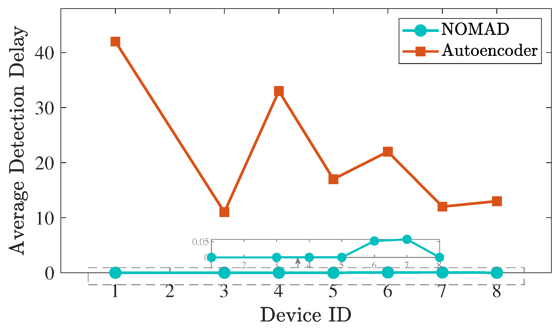
5.1. N-BaIoT Dataset

We evaluate the proposed NOMAD algorithms using the N-BaIoT dataset, that consists of real IoT data traffic observations, including botnet attacks. These data are collected from nine IoT devices, including doorbells, thermostats, baby monitors, etc., infected by the Mirai and BASHLITE malware [36,44]. Here, we only consider the Mirai attack dataset. The benign and attack datasets for each device are composed of 115 features summarizing traffic statistics over different temporal windows. The dataset is collected for each device separately, and lacks a timestamp. The number of instances is varied for each device and attack type. Therefore, we formed the training and testing sets by randomly choosing data instances from each device. To form a network-wide instance for multivariate detection, we stack the chosen instances from nine devices into a single vector of 1035 dimensions. This way, we obtain a nominal training set with N = 10,000 instances. We also build an anomalous training set with $M=5000$ instances for the Ecobee thermostat device (device 3). To test the performance of NOMADs for both known and unknown attack types, we let NOMADs train only on attack data from device 3, and test under two scenarios:

(i)

Device 3 (Ecobee Thermostat) is compromised (known anomaly type);

(ii)

Device 6 (Provision PT-838 security camera) is compromised (unknown anomaly type).

We form the testing data in similar fashion to the training data, assuming that the respective device is compromised and starts sending malicious traffic at $t=101$. In the NOMAD algorithms, we set the parameters as $k=\gamma =1$, ${\alpha }_1=0.05$, ${\alpha }_2=0.1$.

NOMAD is able to detect the attack with zero detection delay and zero false alarm in all trials in both known and unknown attack scenarios (Figure 2). As for NOMADs that trains also on attack data from device 3, in the known attack scenario, zero detection delay with zero false alarm in all trials is achieved, similar to NOMAD. Figure 2 demonstrates the average performance of both variants for the detection of attack when device 6 is compromised, i.e., an unknown anomaly type for NOMADs. In this scenario, although NOMADs is not trained on this anomaly type, it is still able to detect it, yet with a slight degradation in performance as compared to the known anomaly case. The detection of unknown anomaly types by NOMADs is not guaranteed to happen in general, and it depends on whether the anomalous observations are relatively similar to the nominal dataset or to the anomalous dataset. Both the unsupervised and supervised NOMAD algorithms achieve much quicker detection than the state-of-the-art sequential detectors NEWMA [34] and nearest neighbor (NN) based change detection methods in [30]. NEWMA [34] is an online and multivariate change detection algorithm that is based on the exponential weighted moving average method. The NN method [30] is based on the two-sample test method proposed in [45,46], which, given two sample sets, determines whether they belong to the same distribution by employing a kNN similarity graph. We tried different window sizes for NEWMA and NN, and found the optimum for both to be 50.

We also compare the performance of NOMAD with the deep auto encoder-based detection method, that was proposed in the paper that presented the N-BaIoT dataset [36], as they both train only on the nominal data. The auto encoder method marks each observation instance as nominal or anomalous, and employs majority voting on a moving window of size $w{s}^{*}$ (to control the false positive rate), raising alarm only if the majority of instances within the window are marked as anomalous. Due to its window-based majority rule, the sample detection delay (i.e., the number of anomalous instances observed before the detection) is at least $\lfloor \frac{w{s}^{*}}{2}\rfloor +1$. Whereas, the sequential nature of NOMAD enables the immediate detection together with zero false alarm, as demonstrated in Figure 3 and Figure 4. Following the analysis in [36] for each device, the sample detection delay and the false positive rate of both methods are compared in Figure 3 and Figure 4, respectively. The optimum window sizes reported in [36] for each device are used for the auto encoder method.

Online Learning Scheme (NOMADo): Here, we present the experiment results to demonstrate the practical advantage of the self-supervised online learning framework NOMADo, proposed in Section 4.4. Following the experiments of Section 5.1, we train the algorithms on the nominal data and anomaly data for a specific attack type. For the N-BaIoT dataset, we repeat the Scenario 2 test, in which device 6 (Provision PT-838 security camera) starts sending malicious traffic while only the attack data from device 3 is used to train NOMADs.

Figure 5 shows the average detection delay by NOMADs for a constant false alarm rate of $0.01$, versus the number of the data points from the new anomaly type added to the anomaly training set. As the number of confirmed instances added to the anomaly training set grows, NOMADs detection delay decreases. The confirmation can be through either a human expert or a sufficiently high decision threshold for NOMAD that avoids false alarms, as explained in Section 4.4. Although in general NOMADs may not detect an unknown anomaly at the first encounter, it is able to detect the unknown anomaly in the N-BaIoT dataset at the first encounter with an average delay of $0.79$, and the average delay converges to zero as the training set is enhanced with instances from the new anomaly type. In this way, NOMADo, in general, detects the unknown anomaly types through NOMAD, and over time learns the pattern of new anomalies, and improves its detection performance through NOMADs.

5.2. Cyber Physical System: SWaT Data Set

We further analyze our algorithm on an operational test bed setup called the secure water treatment (SWaT) system. The data were collected with Singapore’s Public Utility Board to ensure the resemblance of the system to real systems in the field. The data were collected for 11 days with the system being operational for the entire day. During the last 4 days of the data collection process, a total of 36 attacks were launched with cyber physical sensors, such as water level sensors, actuators, and valves as the primary target points. The attacks did not conform to any pattern with respect to intent or lasting duration, with some attacks lasting for an entire hour. The details of the SWaT system is publicly available on its website (https://itrust.sutd.edu.sg/testbeds/secure-water-treatment-swat/, last accessed on 23 April 2023). The SWaT dataset is a high dimensional, multivariate system with data streaming from 51 sensors and actuators. In all, 496,800 samples were collected under normal working conditions and another 449,919 samples were collected with the system under attack. Our proposed NOMAD algorithm is compared with several other algorithms in

Table 2. Performance comparison of NOMAD on the SWaT dataset with various algorithms.

Algorithm	Pre	Rec	F1
PCA	24.92	21.63	0.23
KNN	7.83	7.83	0.08
FB	10.17	10.17	0.10
AE	72.63	52.63	0.61
EGAN	40.57	67.73	0.51
MAD-GAN	98.97	63.74	0.77
BeatGAN	64.01	87.46	73.92
DAGMM	89.92	57.84	70.40
Ours	99.76	64.7	0.783

: the PCA-based method in [32], KNN-based method in [33], feature bagging (FB) [35], auto encoder-based (AE) method in [37], EGAN [38], multivariate generative adversarial network based anomaly detection method (MAD-GAN) [39], BeatGAN [47], and deep auto encoding Gaussian mixture model (DAGMM) [48]. As seen in the table, we achieve the best result in terms of precision, recall, and F1 score.

6. Conclusions

In this paper, we proposed an algorithm, called NOMAD, that is suitable for quick and accurate anomaly detection in high dimensional systems that require the multivariate (i.e., joint) monitoring of system components. Our proposed anomaly detection method is generic and applicable to various contexts as it does not assume specific data types, probability distributions, and anomaly types. It only requires a nominal training set. We analyzed its computational complexity and asymptotic false alarm rate, that yielded a closed-form expression for setting its decision threshold. We also showed how to benefit from available anomalous data (NOMADs), and presented an online learning scheme (NOMADo) that detects unknown anomaly types, and over time improves its performance by learning on-the-fly. We evaluated the performance of our method in the context of cyber-attack detection using real datasets. The experiments verified the advantage of the proposed online learning method, and also showed that the proposed NOMAD methods significantly outperform the state-of-the-art anomaly detection methods in terms of detection accuracy, average detection delay, and false alarm rate. The proposed algorithms assume a static nominal behavior and a static set of data dimensions. Extending it to dynamic settings with changing nominal behavior remains an important future research direction.

References

1. Chandola, V.; Banerjee, A.; Kumar, V. Anomaly detection: A survey. ACM Comput. Surv. (CSUR) 2009, 41, 15. [Google Scholar] [CrossRef]
2. Cui, M.; Wang, J.; Yue, M. Machine Learning-Based Anomaly Detection for Load Forecasting Under Cyberattacks. IEEE Trans. Smart Grid 2019, 10, 5724–5734. [Google Scholar] [CrossRef]
3. Xiang, Y.; Li, K.; Zhou, W. Low-rate DDoS attacks detection and traceback by using new information metrics. IEEE Trans. Inf. Forensics Secur. 2011, 6, 426–437. [Google Scholar] [CrossRef]
4. Doshi, K.; Yilmaz, Y.; Uludag, S. Timely detection and mitigation of stealthy DDoS attacks via IoT networks. IEEE Trans. Depend. Secur. Comput. 2021, 18, 2164–2176. [Google Scholar] [CrossRef]
5. Elnaggar, R.; Chakrabarty, K.; Tahoori, M.B. Hardware trojan detection using changepoint-based anomaly detection techniques. IEEE Trans. Very Large Scale Integr. (VLSI) Syst. 2019, 27, 2706–2719. [Google Scholar] [CrossRef]
6. Zhang, H.; Liu, J.; Kato, N. Threshold tuning-based wearable sensor fault detection for reliable medical monitoring using Bayesian network model. IEEE Syst. J. 2018, 12, 1886–1896. [Google Scholar] [CrossRef]
7. Doshi, K.; Yilmaz, Y. Online anomaly detection in surveillance videos with asymptotic bound on false alarm rate. Pattern Recognit. 2021, 114, 107865. [Google Scholar] [CrossRef]
8. Matthews, B. Automatic Anomaly Detection with Machine Learning. 2019. Available online: https://ntrs.nasa.gov/citations/20190030491 (accessed on 23 April 2023).
9. Haydari, A.; Yilmaz, Y. RSU-based online intrusion detection and mitigation for VANET. Sensors 2022, 22, 7612. [Google Scholar] [CrossRef]
10. Mozaffari, M.; Doshi, K.; Yilmaz, Y. Real-Time Detection and Classification of Power Quality Disturbances. Sensors 2022, 22, 7958. [Google Scholar] [CrossRef]
11. Doshi, K.; Abudalou, S.; Yilmaz, Y. Reward Once, Penalize Once: Rectifying Time Series Anomaly Detection. In Proceedings of the 2022 International Joint Conference on Neural Networks (IJCNN), Padua, Italy, 18–23 July 2022; pp. 1–8. [Google Scholar]
12. Hundman, K.; Constantinou, V.; Laporte, C.; Colwell, I.; Soderstrom, T. Detecting spacecraft anomalies using lstms and non-parametric dynamic thresholding. In Proceedings of the 24th ACM SIGKDD International Conference on Knowledge Discovery & Data Mining, London, UK, 19–23 August 2018; pp. 387–395. [Google Scholar]
13. Chatillon, P.; Ballester, C. History-based anomaly detector: An adversarial approach to anomaly detection. arXiv 2019, arXiv:1912.11843. [Google Scholar]
14. Ravanbakhsh, M. Generative Models for Novelty Detection: Applications in abnormal event and situational change detection from data series. arXiv 2019, arXiv:1904.04741. [Google Scholar]
15. Sabokrou, M.; Khalooei, M.; Fathy, M.; Adeli, E. Adversarially learned one-class classifier for novelty detection. In Proceedings of the IEEE Conference on Computer Vision and Pattern Recognition, Salt Lake City, UT, USA, 18–22 June 2018; pp. 3379–3388. [Google Scholar]
16. Kirkpatrick, J.; Pascanu, R.; Rabinowitz, N.; Veness, J.; Desjardins, G.; Rusu, A.A.; Milan, K.; Quan, J.; Ramalho, T.; Grabska-Barwinska, A.; et al. Overcoming catastrophic forgetting in neural networks. Proc. Natl. Acad. Sci. USA 2017, 114, 3521–3526. [Google Scholar] [CrossRef]
17. Doshi, K.; Yilmaz, Y. Continual learning for anomaly detection in surveillance videos. In Proceedings of the IEEE/CVF Conference on Computer Vision and Pattern Recognition Workshops, Seattle, WA, USA, 14–19 June 2020; pp. 254–255. [Google Scholar]
18. Banerjee, T.; Firouzi, H.; Hero III, A.O. Quickest detection for changes in maximal knn coherence of random matrices. arXiv 2015, arXiv:1508.04720. [Google Scholar] [CrossRef]
19. Soltan, S.; Mittal, P.; Poor, H.V. BlackIoT: IoT Botnet of high wattage devices can disrupt the power grid. In Proceedings of the 27th {USENIX} Security Symposium ({USENIX} Security 18), Baltimore, MD, USA, 15–17 August 2018; pp. 15–32. [Google Scholar]
20. Steinwart, I.; Hush, D.; Scovel, C. A classification framework for anomaly detection. J. Mach. Learn. Res. 2005, 6, 211–232. [Google Scholar]
21. Lee, W.; Xiang, D. Information-theoretic measures for anomaly detection. In Proceedings of the Security and Privacy, 2001, S&P 2001, 2001 IEEE Symposium, Oakland, CA, USA, 14–16 May 2000; pp. 130–143. [Google Scholar]
22. Page, E.S. Continuous inspection schemes. Biometrika 1954, 41, 100–115. [Google Scholar] [CrossRef]
23. Moustakides, G.V. Optimal stopping times for detecting changes in distributions. Ann. Stat. 1986, 14, 1379–1387. [Google Scholar] [CrossRef]
24. Mei, Y. Efficient scalable schemes for monitoring a large number of data streams. Biometrika 2010, 97, 419–433. [Google Scholar] [CrossRef]
25. Banerjee, T.; Hero, A.O. Quickest hub discovery in correlation graphs. In Proceedings of the Signals, Systems and Computers, 2016 50th Asilomar Conference, Pacific Grove, CA, USA, 6–9 November 2016; pp. 1248–1255. [Google Scholar]
26. Hero, A.O. Geometric entropy minimization (GEM) for anomaly detection and localization. In Advances in Neural Information Processing Systems; Curran Associates Inc.: New York, NY, USA, 2007; pp. 585–592. [Google Scholar]
27. Sricharan, K.; Hero, A.O. Efficient anomaly detection using bipartite k-NN graphs. In Advances in Neural Information Processing Systems; Curran Associates Inc.: New York, NY, USA, 2011; pp. 478–486. [Google Scholar]
28. Scott, C.D.; Nowak, R.D. Learning minimum volume sets. J. Mach. Learn. Res. 2006, 7, 665–704. [Google Scholar]
29. Zhao, M.; Saligrama, V. Anomaly detection with score functions based on nearest neighbor graphs. In Advances in Neural Information Processing Systems; Curran Associates Inc.: New York, NY, USA, 2009; pp. 2250–2258. [Google Scholar]
30. Chen, H. Sequential change-point detection based on nearest neighbors. Ann. Stat. 2019, 47, 1381–1407. [Google Scholar] [CrossRef]
31. Zambon, D.; Alippi, C.; Livi, L. Concept drift and anomaly detection in graph streams. IEEE Trans. Neural Netw. Learn. Syst. 2018, 29, 5592–5605. [Google Scholar] [CrossRef]
32. Zhao, Y.; Nasrullah, Z.; Li, Z. Pyod: A python toolbox for scalable outlier detection. arXiv 2019, arXiv:1901.01588. [Google Scholar]
33. Angiulli, F.; Pizzuti, C. Fast outlier detection in high dimensional spaces. In European Conference on Principles of Data Mining and Knowledge Discovery; Springer: Berlin/Heidelberg, Germany, 2002; pp. 15–27. [Google Scholar]
34. Keriven, N.; Garreau, D.; Poli, I. NEWMA: A new method for scalable model-free online change-point detection. IEEE Trans. Signal Process. 2020, 68, 3515–3528. [Google Scholar] [CrossRef]
35. Lazarevic, A.; Kumar, V. Feature bagging for outlier detection. In Proceedings of the Eleventh ACM SIGKDD International Conference on Knowledge Discovery in Data Mining, Chicago, IL, USA, 21–24 August 2005; pp. 157–166. [Google Scholar]
36. Meidan, Y.; Bohadana, M.; Mathov, Y.; Mirsky, Y.; Shabtai, A.; Breitenbacher, D.; Elovici, Y. N-BaIoT—Network-Based Detection of IoT Botnet Attacks Using Deep Autoencoders. IEEE Pervasive Comput. 2018, 17, 12–22. [Google Scholar] [CrossRef]
37. Sakurada, M.; Yairi, T. Anomaly detection using autoencoders with nonlinear dimensionality reduction. In Proceedings of the MLSDA 2014 2nd Workshop on Machine Learning for Sensory Data Analysis, Gold Coast, Australia, 2 December 2014; pp. 4–11. [Google Scholar]
38. Zenati, H.; Foo, C.S.; Lecouat, B.; Manek, G.; Chandrasekhar, V.R. Efficient gan-based anomaly detection. arXiv 2018, arXiv:1802.06222. [Google Scholar]
39. Li, D.; Chen, D.; Jin, B.; Shi, L.; Goh, J.; Ng, S.K. Mad-gan: Multivariate anomaly detection for time series data with generative adversarial networks. In International Conference on Artificial Neural Networks; Springer: Cham, Switzerland, 2019; pp. 703–716. [Google Scholar]
40. Lorden, G. Procedures for reacting to a change in distribution. Ann. Math. Stat. 1971, 42, 1897–1908. [Google Scholar] [CrossRef]
41. Chen, G.H.; Shah, D. Explaining the success of nearest neighbor methods in prediction. Found. Trends Mach. Learn. 2018, 10, 337–588. [Google Scholar] [CrossRef]
42. Gu, X.; Akoglu, L.; Rinaldo, A. Statistical Analysis of Nearest Neighbor Methods for Anomaly Detection. In Proceedings of the Advances in Neural Information Processing Systems, Vancouver, BC, Canada, 8–14 December 2019; pp. 10921–10931. [Google Scholar]
43. Muja, M.; Lowe, D.G. Scalable nearest neighbor algorithms for high dimensional data. IEEE Trans. Pattern Anal. Mach. Intell. 2014, 36, 2227–2240. [Google Scholar] [CrossRef]
44. Mirsky, Y.; Doitshman, T.; Elovici, Y.; Shabtai, A. Kitsune: An ensemble of autoencoders for online network intrusion detection. arXiv 2018, arXiv:1802.09089. [Google Scholar]
45. Schilling, M.F. Multivariate two-sample tests based on nearest neighbors. J. Am. Stat. Assoc. 1986, 81, 799–806. [Google Scholar] [CrossRef]
46. Henze, N. A multivariate two-sample test based on the number of nearest neighbor type coincidences. Ann. Stat. 1988, 772–783. [Google Scholar] [CrossRef]
47. Zhou, B.; Liu, S.; Hooi, B.; Cheng, X.; Ye, J. BeatGAN: Anomalous Rhythm Detection using Adversarially Generated Time Series. Proc. IJCAI 2019, 2019, 4433–4439. [Google Scholar]
48. Zong, B.; Song, Q.; Min, M.R.; Cheng, W.; Lumezanu, C.; Cho, D.; Chen, H. Deep autoencoding gaussian mixture model for unsupervised anomaly detection. In Proceedings of the International Conference on Learning Representations, Vancouver, BC, Canada, 30 April–3 May 2018. [Google Scholar]
49. Stoyan, D.; Kendall, W.S.; Chiu, S.N.; Mecke, J. Stochastic Geometry and Its Applications; John Wiley & Sons: Hoboken, NJ, USA, 2013. [Google Scholar]
50. Basseville, M.; Nikiforov, I.V. Detection of Abrupt Changes: Theory and Application; Prentice Hall: Englewood Cliffs, NJ, USA, 1993; Volume 104. [Google Scholar]
51. Scott, T.C.; Fee, G.; Grotendorst, J. Asymptotic series of generalized Lambert W function. ACM Commun. Comput. Algebra 2014, 47, 75–83. [Google Scholar] [CrossRef]
52. Agresti, A. An Introduction to Categorical Data Analysis; Wiley: Hoboken, NJ, USA, 2018. [Google Scholar]
Figure 1. Comparison between the performance of NOMAD by computing the exact kNN distance and approximating the kNN distance.
Electronics 12 01971 g001
Figure 2. Performance comparison between NOMAD, NOMADs, and the existing methods in the unknown attack scenario for the N-BaIoT dataset.
Electronics 12 01971 g002
Figure 3. Average detection delay of the auto encoder method [36] and NOMAD in terms of the number of samples for each device attack scenario.
Electronics 12 01971 g003
Figure 4. False positive rate of the auto encoder method [36] and NOMAD for each device attack scenario.
Electronics 12 01971 g004
Figure 5. Average detection delay of NOMADs vs. the number of the new anomaly instances added to the training set for the N-BaIoT dataset.
Electronics 12 01971 g005