

Free-Viewpoint Navigation of Indoor Scene with 360° Field of View

Abstract
:1. Introduction
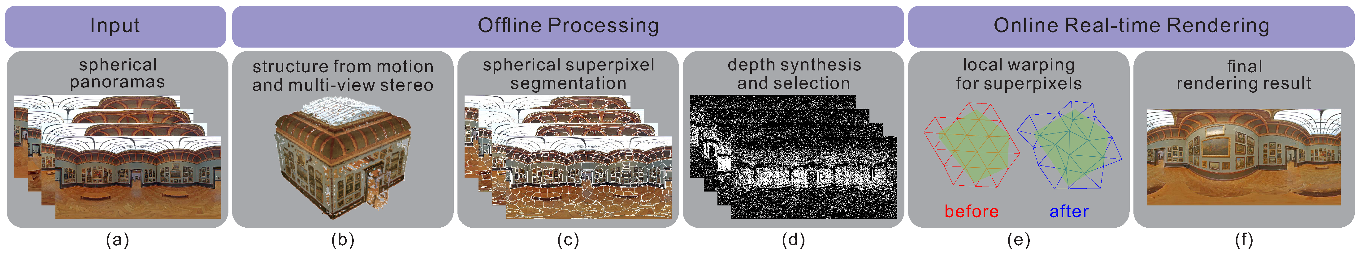
- We propose a panoramic image-based rendering algorithm for free-viewpoint navigation of indoor scenes. Unlike previous methods, our method does not assume that a novel view lies on the line connecting input views and thus can let the user freely explore the indoor scene.
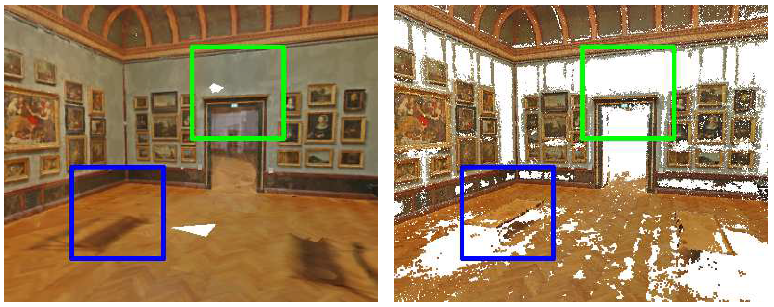
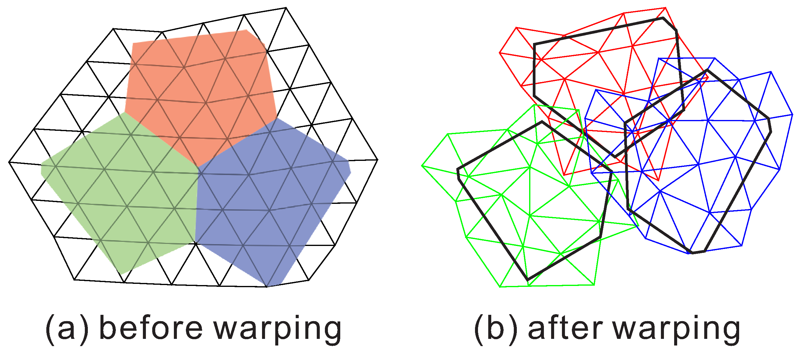
- We explore a spherical superpixel-based per-view representation and locally warp each superpixel individually for novel view synthesis, which can prevent us from occlusion problems and artefacts.
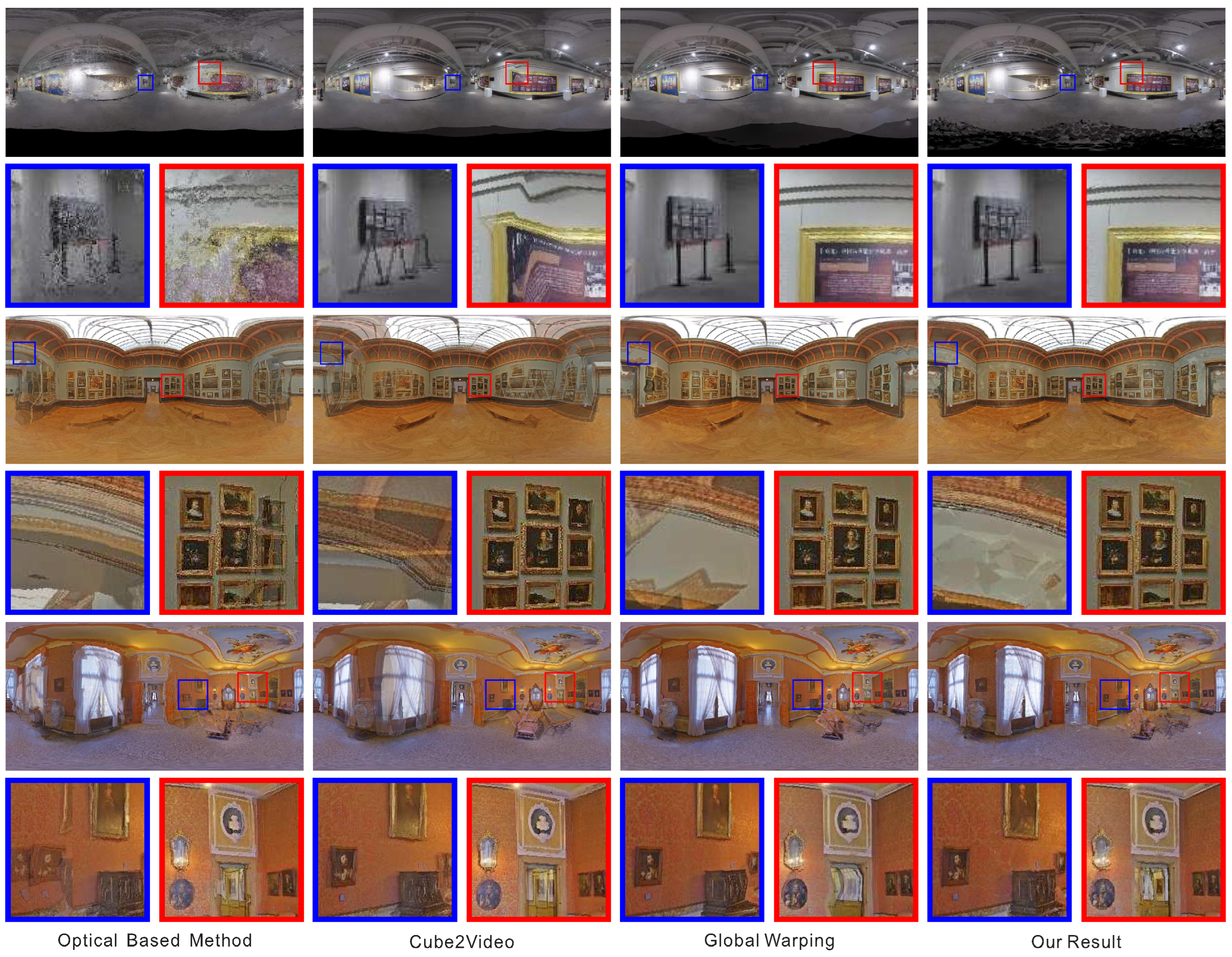
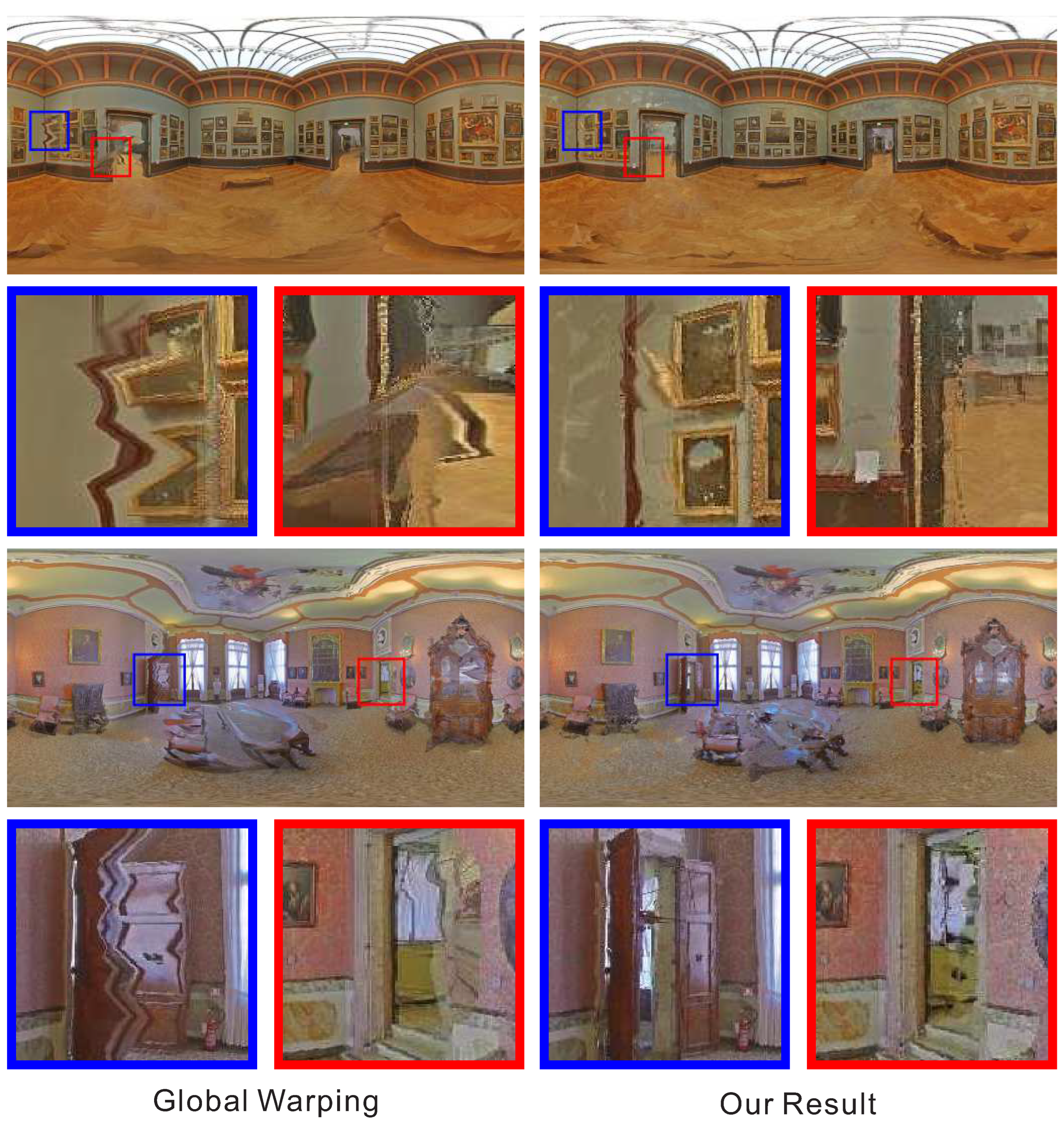
- We have tested our method on downloaded and self-captured panoramic datasets. Experimental results show that our method achieves better performance compared with baselines.
2. Related Work
2.1. 3D Reconstruction from Panoramas
2.2. Planar Image Based Rendering
2.3. Panoramic Image Based Rendering
2.4. Free-Viewpoint Navigation
3. Overview
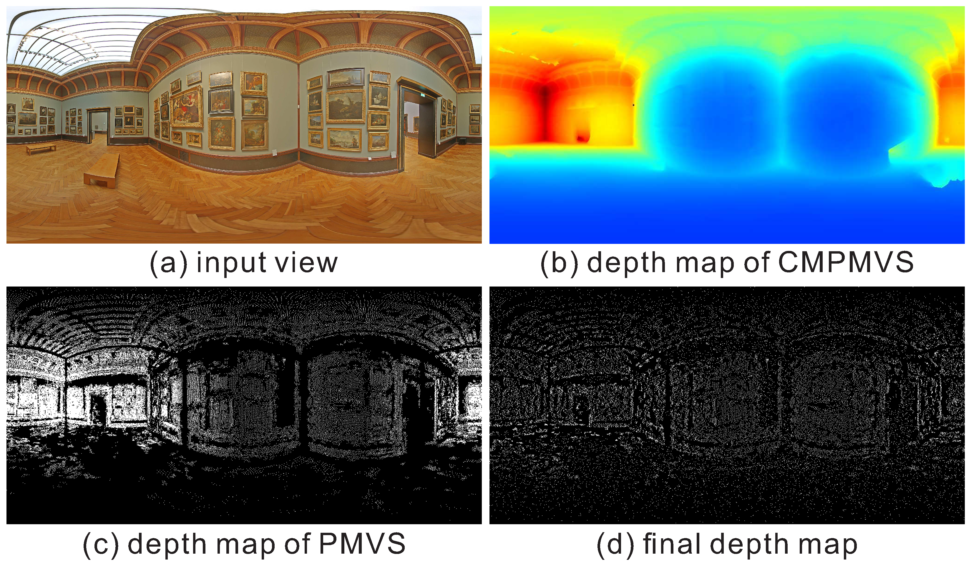
4. Depth Map Generation
4.1. Structure from Motion
4.2. Multi-View Stereo
4.3. Depth Synthesis and Selection
5. Local Warping and Rendering
5.1. Superpixel Local Warping
5.2. Real-Time Rendering
6. Experimental Results
6.1. Implementation Details
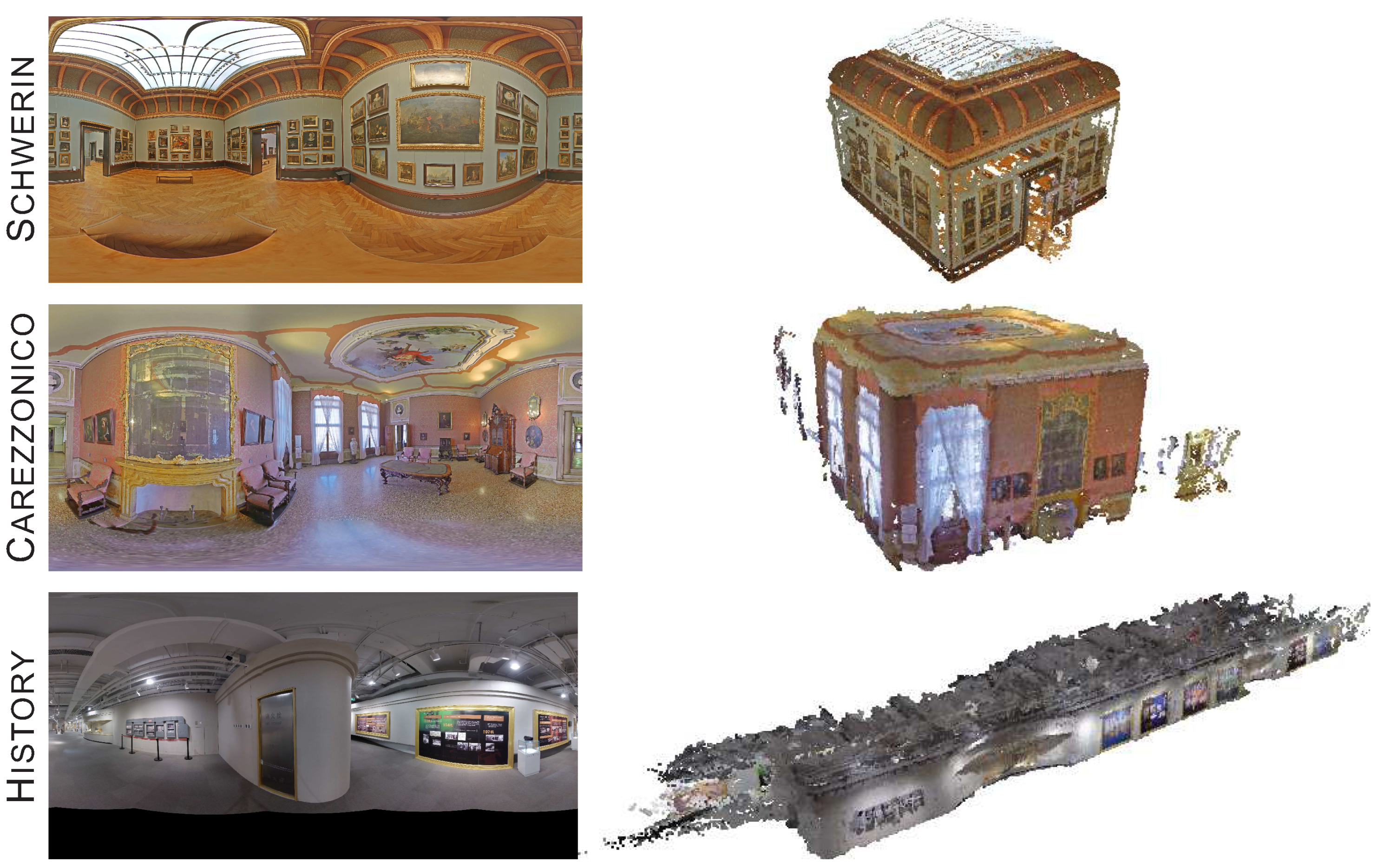
6.2. Dataset
6.3. Discussion
6.4. Limitation
7. Conclusions
Author Contributions
Funding
Data Availability Statement
Conflicts of Interest
References
- Greene, N. Environment Mapping and Other Applications of World Projections. IEEE Comput. Graph. Appl. 1986, 6, 21–29. [Google Scholar] [CrossRef]
- Chen, S.E. QuickTime VR: An Image-based Approach to Virtual Environment Navigation. In Proceedings of the 22nd Annual Conference on Computer Graphics and Interactive Techniques, Los Angeles, CA, USA, 6–11 August 1995; pp. 29–38. [Google Scholar]
- Uyttendaele, M.; Criminisi, A.; Kang, S.B.; Winder, S.; Szeliski, R.; Hartley, R. Image-based interactive exploration of real-world environments. IEEE Comput. Graph. Appl. 2004, 24, 52–63. [Google Scholar] [CrossRef]
- Anguelov, D.; Dulong, C.; Filip, D.; Frueh, C.; Lafon, S.; Lyon, R.; Ogale, A.; Vincent, L.; Weaver, J. Google Street View: Capturing the World at Street Level. Computer 2010, 43, 32–38. [Google Scholar] [CrossRef]
- Google Arts and Culture. Available online: https://artsandculture.google.com (accessed on 19 April 2023).
- Chan, Y.-F.; Fok, M.-H.; Fu, C.-W.; Heng, P.-A.; Wong, T.-T. A panoramic-based walkthrough system using real photos. In Proceedings of the Pacific Conference Computer Graphics and Application, Seoul, Republic of Korea, 5–7 October 1999; pp. 231–240. [Google Scholar]
- Kolhatkar, S.; Laganière, R. Real-Time Virtual Viewpoint Generation on the GPU for Scene Navigation. In Proceedings of the Canadian Conference Computer and Robot Vision, Ottawa, ON, Canada, 31 May–2 June 2010; pp. 55–62. [Google Scholar]
- Zhao, Q.; Wan, L.; Feng, W.; Zhang, J.; Wong, T. Cube2Video: Navigate Between Cubic Panoramas in Real-Time. IEEE Trans. Multimed. 2013, 15, 1745–1754. [Google Scholar] [CrossRef]
- Kawai, N.; Audras, C.; Tabata, S.; Matsubara, T. Panorama Image Interpolation for Real-time Walkthrough. In Proceedings of the ACM SIGGRAPH Posters, Anaheim, CA, USA, 24–28 July 2016; pp. 33:1–33:2. [Google Scholar]
- Andersen, D.; Popescu, V. HMD-Guided Image-Based Modeling and Rendering of Indoor Scenes. In Proceedings of the Virtual Reality and Augmented Reality, London, UK, 22–23 October 2018; pp. 73–93. [Google Scholar]
- Siu, A.M.K.; Lau, R.W.H. Image registration for image-based rendering. IEEE Trans. Image Process. 2005, 14, 241–252. [Google Scholar] [CrossRef]
- Dai, F.; Zhu, C.; Ma, Y.; Cao, J.; Zhao, Q.; Zhang, Y. Freely Explore the Scene with 360° Field of View. In Proceedings of the 2019 IEEE Conference on Virtual Reality and 3D User Interfaces (VR), Osaka, Japan, 23–27 March 2019. [Google Scholar]
- Zhao, Q.; Dai, F.; Ma, Y.; Wan, L.; Zhang, J.; Zhang, Y. Spherical Superpixel Segmentation. IEEE Trans. Multimed. 2018, 20, 1406–1417. [Google Scholar] [CrossRef]
- Zioulis, N.; Karakottas, A.; Zarpalas, D.; Daras, P. OmniDepth: Dense Depth Estimation for Indoors Spherical Panoramas. In Proceedings of the European Conference on Computer Vision, Munich, Germany, 8–14 September 2018; pp. 453–471. [Google Scholar]
- Zioulis, N.; Karakottas, A.; Zarpalas, D.; Alvarez, F.; Daras, P. Spherical View Synthesis for Self-Supervised 360 Depth Estimation. arXiv 2019, arXiv:1909.08112v1. [Google Scholar]
- Lai, P.K.; Xie, S.; Lang, J.; Laganière, R. Real-Time Panoramic Depth Maps from Omni-directional Stereo Images for 6 DoF Videos in Virtual Reality. In Proceedings of the IEEE Conference on Virtual Reality and 3D User Interfaces (VR), Osaka, Japan, 23–27 March 2019; pp. 405–412. [Google Scholar]
- Wang, F.E.; Hu, H.N.; Cheng, H.T.; Lin, J.T.; Yang, S.T.; Shih, M.L.; Chu, H.K.; Sun, M. Self-supervised Learning of Depth and Camera Motion from 360 Videos. In Proceedings of the Asia Conference on Computer Vision, Perth, Australia, 2–6 December 2018; pp. 53–68. [Google Scholar]
- Kim, H.; Hilton, A. 3D Scene Reconstruction from Multiple Spherical Stereo Pairs. Int. J. Comput. Vis. 2013, 104, 94–116. [Google Scholar] [CrossRef]
- da Silveira, T.L.T.; Jung, C.R. Dense 3D Scene Reconstruction from Multiple Spherical Images for 3-DoF+ VR Applications. In Proceedings of the IEEE Conference on Virtual Reality and 3D User Interfaces (VR), Osaka, Japan, 23–27 March 2019; pp. 9–18. [Google Scholar]
- Peng, Z.; Hou, S.; Yuan, Y. EPAR: An Efficient and Privacy-Aware Augmented Reality Framework for Indoor Location-Based Services. In Proceedings of the 2022 IEEE/RSJ International Conference on Intelligent Robots and Systems (IROS), Hamburg, Germany, 22–25 May 2022; pp. 8948–8955. [Google Scholar]
- Shum, H.Y.; Chan, S.C.; Kang, S.B. Image-Based Rendering; Springer Science & Business Media: Berlin/Heidelberg, Germany, 2008. [Google Scholar]
- Chaurasia, G.; Duchene, S.; Sorkine-Hornung, O.; Drettakis, G. Depth Synthesis and Local Warps for Plausible Image-based Navigation. ACM Trans. Graph. 2013, 32, 30:1–30:12. [Google Scholar] [CrossRef]
- Hedman, P.; Ritschel, T.; Drettakis, G.; Brostow, G. Scalable Inside-Out Image-Based Rendering. ACM Trans. Graph. 2016, 35, 231:1–231:11. [Google Scholar] [CrossRef]
- Hedman, P.; Philip, J.; Price, T.; Frahm, J.M.; Drettakis, G.; Brostow, G. Deep Blending for Free-viewpoint Image-based Rendering. ACM Trans. Graph. 2018, 37, 257:1–257:15. [Google Scholar] [CrossRef]
- Chen, B.; Neubert, B.; Ofek, E.; Deussen, O.; Cohen, M.F. Integrated Videos and Maps for Driving Directions. In Proceedings of the ACM Symposium on User Interface Software and Technology, Victoria, BC, Canada, 4–7 October 2009; pp. 223–232. [Google Scholar]
- Huang, J.; Chen, Z.; Ceylan, D.; Jin, H. 6-DOF VR videos with a single 360-camera. In Proceedings of the IEEE Virtual Reality (VR), Los Angeles, CA, USA, 18–22 March 2017; pp. 37–44. [Google Scholar]
- Levoy, M.; Hanrahan, P. Light Field Rendering. In Proceedings of the 23rd Annual Conference on Computer Graphics and Interactive Techniques, New Orleans, LA, USA, 4–9 August 1996; pp. 31–42. [Google Scholar]
- Birklbauer, C.; Bimber, O. Panorama Light-Field Imaging. Comput. Graph. Forum 2014, 33, 43–52. [Google Scholar] [CrossRef]
- Taguchi, Y.; Agrawal, A.; Veeraraghavan, A.; Ramalingam, S.; Raskar, R. Axial-cones: Modeling Spherical Catadioptric Cameras for Wide-angle Light Field Rendering. ACM Trans. Graph. 2010, 29, 172:1–172:8. [Google Scholar] [CrossRef]
- Krolla, B.; Diebold, M.; Goldlücke, B.; Stricker, D. Spherical Light Fields. In Proceedings of the British Machine Vision Conference, Nottingham, UK, 1–5 September 2014. [Google Scholar]
- Snavely, N.; Seitz, S.M.; Szeliski, R. Photo Tourism: Exploring Photo Collections in 3D. ACM Trans. Graph. 2006, 25, 835–846. [Google Scholar] [CrossRef]
- Furukawa, Y.; Ponce, J. Accurate, Dense, and Robust Multiview Stereopsis. IEEE Trans. Pattern Anal. Mach. Intell. 2010, 32, 1362–1376. [Google Scholar] [CrossRef] [PubMed]
- Gluckman, J.; Nayar, S.K. Ego-motion and omnidirectional cameras. In Proceedings of the International Conference on Computer Vision, Bombay, India, 4–7 January 1998; pp. 999–1005. [Google Scholar]
- Lowe, D.G. Distinctive Image Features from Scale-Invariant Keypoints. Int. J. Comput. Vis. 2004, 60, 91–110. [Google Scholar] [CrossRef]
- Guan, H.; Smith, W.A.P. BRISKS: Binary Features for Spherical Images on a Geodesic Grid. In Proceedings of the IEEE Conference on Computer Vision and Pattern Recognition, Honolulu, HI, USA, 21–26 July 2017; pp. 4886–4894. [Google Scholar]
- Hartley, R.; Zisserman, A. Multiple View Geometry in Computer Vision; Cambridge University Press: Cambridge, UK, 2003. [Google Scholar]
- Scharstein, D.; Szeliski, R. A Taxonomy and Evaluation of Dense Two-Frame Stereo Correspondence Algorithms. Int. J. Comput. Vis. 2002, 47, 7–42. [Google Scholar] [CrossRef]
- Multi-View Stereo: A Tutorial. Found. Trends Comput. Graph. Vis. 2015, 9, 1–148. [CrossRef]
- Jancosek, M.; Pajdla, T. Multi-view reconstruction preserving weakly-supported surfaces. In Proceedings of the IEEE Conference on Computer Vision and Pattern Recognition, Washington, DC, USA, 20–25 June 2011; pp. 3121–3128. [Google Scholar]
- Achanta, R.; Shaji, A.; Smith, K.; Lucchi, A.; Fua, P.; Süsstrunk, S. SLIC Superpixels Compared to State-of-the-Art Superpixel Methods. IEEE Trans. Pattern Anal. Mach. Intell. 2012, 34, 2274–2282. [Google Scholar] [CrossRef]
- Liu, F.; Gleicher, M.; Jin, H.; Agarwala, A. Content-preserving Warps for 3D Video Stabilization. ACM Trans. Graph. 2009, 28, 44:1–44:9. [Google Scholar] [CrossRef]
- Buehler, C.; Bosse, M.; McMillan, L.; Gortler, S.; Cohen, M. Unstructured Lumigraph Rendering. In Proceedings of the 28th Annual Conference on Computer Graphics and Interactive Techniques, Los Angeles, CA, USA, 12–17 August 2001; pp. 425–432. [Google Scholar]
- Chen, Y.; Davis, T.A.; Hager, W.W.; Rajamanickam, S. Algorithm 887: CHOLMOD, supernodal sparse Cholesky factorization and update/downdate. ACM Trans. Math. Softw. 2008, 35, 22. [Google Scholar] [CrossRef]
- Tang, C.; Tan, P. BA-Net: Dense Bundle Adjustment Networks. In Proceedings of the International Conference on Learning Representations, New Orleans, LA, USA, 6–9 May 2019. [Google Scholar]
- Huang, P.; Matzen, K.; Kopf, J.; Ahuja, N.; Huang, J. DeepMVS: Learning Multi-view Stereopsis. In Proceedings of the IEEE Conference on Computer Vision and Pattern Recognition, Salt Lake City, UT, USA, 18–23 June 2018; pp. 2821–2830. [Google Scholar]
- Liu, M.; He, X.; Salzmann, M. Geometry-Aware Deep Network for Single-Image Novel View Synthesis. In Proceedings of the IEEE Conference on Computer Vision and Pattern Recognition, Salt Lake City, UT, USA, 18–23 June 2018; pp. 4616–4624. [Google Scholar]


| Scene Name | ♯ Input Views | ♯ Reconstructed Points |
|---|---|---|
| Schwerin | 9 | 176,999 |
| Carezzonico | 11 | 152,429 |
| History | 97 | 1,106,558 |
Disclaimer/Publisher’s Note: The statements, opinions and data contained in all publications are solely those of the individual author(s) and contributor(s) and not of MDPI and/or the editor(s). MDPI and/or the editor(s) disclaim responsibility for any injury to people or property resulting from any ideas, methods, instructions or products referred to in the content. |
© 2023 by the authors. Licensee MDPI, Basel, Switzerland. This article is an open access article distributed under the terms and conditions of the Creative Commons Attribution (CC BY) license (https://creativecommons.org/licenses/by/4.0/).
Share and Cite
Xu, H.; Zhao, Q.; Ma, Y.; Wang, S.; Yan, C.; Dai, F. Free-Viewpoint Navigation of Indoor Scene with 360° Field of View. Electronics 2023, 12, 1954. https://doi.org/10.3390/electronics12081954
Xu H, Zhao Q, Ma Y, Wang S, Yan C, Dai F. Free-Viewpoint Navigation of Indoor Scene with 360° Field of View. Electronics. 2023; 12(8):1954. https://doi.org/10.3390/electronics12081954
Chicago/Turabian StyleXu, Hang, Qiang Zhao, Yike Ma, Shuai Wang, Chenggang Yan, and Feng Dai. 2023. "Free-Viewpoint Navigation of Indoor Scene with 360° Field of View" Electronics 12, no. 8: 1954. https://doi.org/10.3390/electronics12081954